Models and Strategies for Variants of the Job Shop Scheduling Problem

Abstract

Recently, a variety of constraint programming and Boolean satisfiability approaches to scheduling problems have been introduced. They have in common the use of relatively simple propagation mechanisms and an adaptive way to focus on the most constrained part of the problem. In some cases, these methods compare favorably to more classical constraint programming methods relying on propagation algorithms for global unary or cumulative resource constraints and dedicated search heuristics. In particular, we described an approach that combines restarting, with a generic adaptive heuristic and solution guided branching on a simple model based on a decomposition of disjunctive constraints.

In this paper, we introduce an adaptation of this technique for an important subclass of job shop scheduling problems (JSPs), where the objective function involves minimization of earliness/tardiness costs. We further show that our technique can be improved by adding domain specific information for one variant of the JSP (involving time lag constraints). In particular we introduce a dedicated greedy heuristic, and an improved model for the case where the maximal time lag is 0 (also referred to as no-wait JSPs).

1 Introduction

Scheduling problems come in a wide variety and it is natural to think that methods specifically engineered for each variant would have the best performance. However, it was recently shown this is not always true. Tamura et al. introduced an encoding of disjunctive and precedence constraints into conjunctive normal form formulae [22]. Thanks to this reformulation they were the first to report optimality proofs for all open shop scheduling instances from three widely studied benchmarks. Similarly the hybrid CP/SAT solver lazy-FD [10] was shown to be extremely effective on Resource-Constrained Project scheduling (RCPSP) [21].

Previously, we introduced an approach for open and job shop problems with a variety of extra constraints [12, 13] using simple reified binary disjunctive constraints combined with a number of generic SAT and AI techniques: weighted degree variable ordering [5], solution guided value ordering [3], geometric restarting [25] and nogood recording from restarts [15]. It appears that the weighted degree heuristic efficiently detects the most constrained parts of the problem, focusing search on a fraction of the variables.

The simplicity of this approach makes it easy to adapt to various constraints and objective functions. One type of objective function that has proven troublesome for traditional CP scheduling techniques involves minimizing the sum of earliness/tardiness costs, primarily due to the weak propagation of the sum objective [8]. In this paper we show how our basic JSP model can be adapted to handle this objective. Experimental results reveal that our approach is competitive with the state of the art on the standard benchmarks from the literature.

Moreover, we introduce two refinements of our approach for problems with maximum time lags between consecutive tasks, where we incorporate domain specific information to boost performance. These time lag constraints, although conceptually very simple, change the nature of the problem dramatically. For instance, it is not trivial to find a feasible schedule even if we do not take into account any bound on the total makespan (unless scheduling jobs back to back). This has several negative consequences. Firstly, it is not possible to obtain a trivial upper bound of reasonable quality may be found by sequencing the tasks in some arbitrary order. The only obvious upper bound is to sequence the jobs consecutively. Secondly, since relaxing the makespan constraint is not sufficient to make the problem easy, our approach can have difficulty finding a feasible solution for large makespans, even though it is very effective when given a tighter upper bound. However because the initial upper bound is so poor, even an exploration by dichotomy of the objective variable’s domain can take a long time.

We introduce a simple search strategy which, when given a large enough upper bound on the makespan, guarantees a limited amount of backtracking whilst still providing good quality solutions. This simple strategy, used as an initial step, greatly improves the performance of our algorithm on this problem type. We report several new best upper bounds and proofs of optimality on these benchmarks. Moreover, we introduce another improvement in the model of the particular case of No wait JSP where the tasks of each job must be directly consecutive. This variant has been widely studied, and efficient metaheuristics have been proposed recently. We report $5$ new best upper bound, and close $9$ new instances in standard data sets.

Finally, because there are few comparison methods in the literature for problems with strictly positive time lags, we adapted a job shop scheduling model written in Ilog Scheduler by Chris Beck [3], to handle time lag constraints. Our method outperforms this model when time lag constraints are tight (short lags), however when time lags are longer, the Ilog Scheduler model together with geometric restarts and solution guided search is better than our method.

2 Background & Previous work

An $n\times m$ job shop problem (JSP) involves a set of $nm$ tasks ${\cal T}=\{{t_{i}}~{}|~{}1\leq i\leq nm\}$, partitioned into $n$ jobs ${\cal J}=\{{J_{x}}~{}|~{}1\leq x\leq n\}$, that need to be scheduled on $m$ machines ${\cal M}=\{{M_{y}}~{}|~{}1\leq y\leq m\}$. Each job ${J_{x}}\in{\cal J}$ is a set of $m$ tasks ${J_{x}}=\{{t_{(x-1)*m+y}}~{}|~{}1\leq y\leq m\}$. Conversely, each machine ${M_{y}}\in{\cal M}$ denotes a set of $n$ tasks (to run on this machine) such that: ${\cal T}=(\bigcup_{1\leq x\leq n}{J_{x}})=(\bigcup_{1\leq y\leq m}{M_{y}})$.

Each task ${t_{i}}$ has an associated duration, or processing time, ${p_{i}}$. A schedule is a mapping of tasks to time points consistent with sequencing and resource constraints. The former ensure that the tasks of each job run in a predefined order whilst the latter ensure that no two tasks run simultaneously on any given machine. In the rest of the paper, we shall identify each task ${t_{i}}$ with the variable standing for its start time in the schedule. We define the sequencing (2.1) and resource (2.2) constraints in Model 1.

Moreover, we shall consider two objective functions: total makespan, and weighted earliness/tardiness. In the former, we want to minimize the the total duration to run all tasks, that is, $C_{max}=max_{{t_{i}}\in{\cal T}}({t_{i}}+{p_{i}})$ if we assume that we start at time $0$. In the latter, each job ${J_{x}}\in{\cal J}$ has a due date, ${d_{x}}$. There is a linear cost associated with completing a job before its due date, or the tardy completion of a job, with coefficient ${w^{e}_{x}}$ and ${w^{t}_{x}}$, respectively. (Note that these problems differ from Just in Time job shop scheduling problems[2], where each task has a due date.) If ${t_{xm}}$ is the last task of job ${J_{x}}$, then ${t_{xm}}+{p_{xm}}$ is its completion time, hence the cost of a job is then given by: $ET_{sum}=\sum_{{J_{x}}\in{\cal J}}(max({w^{e}_{x}}({d_{x}}-{t_{xm}}-{p_{xm}}),{w^{t}_{x}}({t_{xm}}+{p_{xm}}-{d_{x}})))$

model 1 JSP

$${t_{i}}+{p_{i}}\leq{t_{i+1}} \qquad\forall{J_{x}}\in{\cal J},~{}\forall{t_{i}},{t_{i+1}}\in{J_{x}}$$ (2.1)

$${t_{i}}+{p_{i}}\leq{t_{j}}~{}\vee~{}{t_{j}}+{p_{j}}\leq{t_{i}} \qquad\forall{M_{y}}\in{\cal M},~{}{t_{i}}\neq{t_{j}}\in{M_{y}}$$ (2.2)

2.1 Boolean Model

In previous work [13] we described the following simple model for open shop and job shop scheduling. First, to each task, we associate a variable ${t_{i}}$ taking its value in $[0,\infty]$ that stands for its starting time. Then, for each pair of tasks sharing a machine we introduce a Boolean variable that stands for the relative order of these two tasks. More formally, for each machine ${M_{y}}\in{\cal M}$, and for each pair of tasks ${t_{i}},{t_{j}}\in{M_{y}}$, we have a Boolean variable ${b_{ij}}$, and constraint (2.2) can be reformulated as follows:

$${b_{ij}}=\left\{\begin{array}[]{cl}0\Leftrightarrow{t_{i}}+{p_{i}}\leq{t_{j}}\\ 1\Leftrightarrow{t_{j}}+{p_{j}}\leq{t_{i}}\end{array}\right. \qquad\forall{M_{y}}\in{\cal M},~{}{t_{i}}\neq{t_{j}}\in{M_{y}}$$ (2.5)

Finally, the tasks of each job ${J_{x}}$, are kept in sequence with a set of simple precedence constraints ${t_{i}}+{p_{i}}\leq{t_{i+1}}$ for all ${t_{i}},{t_{i+1}}\in{J_{x}}$.

For $n$ jobs and $m$ machines, this model therefore involves $nm(n-1)/2$ Boolean variables, as many disjunctive constraints, and $n(m-1)$ precedence constraints. Bounds consistency (BC) is maintained on all constraints. Notice that state of the art CP models use instead $m$ global constraints to reason about unary resources. The best known algorithms for filtering unary resources constraints implement the edge finding, not-first/not-last, and detectable precedence rules with a $O(n\log n)$ time complexity [24]. One might therefore expect our model to be less efficient as $n$ grows. However, the quadratic number of constraints – and Boolean variables – required to model a resource in our approach has not proven problematic on the academic benchmarks tested on to date.

2.2 Search Strategy

We refer the reader to [12] for a more detailed description of the default search strategy used for job shop variants, and we give here only a brief overview.

This model does not involve any global constraint associated to a strong propagation algorithm. However, it appears that decomposing resource constraints into binary disjunctive elements is synergetic with adaptive heuristics, and in particular the weighted-degree-based heuristics [5]. (We note that the greater the minimum arity of constraints in a problem, the less discriminatory the weight-degree heuristic can be.) A constraint’s weight is incremented by one each time the constraint causes a failure during search. This weight can then be projected on variables to inform the heuristic choices.

It is sufficient to decide the relative sequencing of the tasks, that is, the value of the Boolean variables standing for disjuncts. Because the domain size of these variables are all equal, we use a slightly modified version of the domain over weighted-degree heuristic, where weights and domain size are taken on the two tasks whose relative ordering is decided by the Boolean variable. Let $w({t_{i}})$ be the number of times search failed while propagating any constraint involving task ${t_{i}}$, and let $min({t_{i}})$ and $max({t_{i}})$ be, respectively, the minimum and maximum starting time of ${t_{i}}$ at any point during search. The next disjunct ${b_{ij}}$ to branch on is the one minimizing the value of:

$$(max({t_{i}})+max({t_{j}})-min({t_{i}})-min({t_{j}})+2)/(w({t_{i}})+w({t_{j}}))$$

A second important aspect is the use of restarts. It has been observed that weighted heuristics also have a good synergy with restarts [11]. Indeed, failures tend to happen at a given depth in the search tree, and therefore on constraints that often do not involve variables corresponding to the first few choices. As a result, early restarts will tend to favor diversification until enough weight has been given to a small set of variables, on which the search will then be focused. We use a geometric restarting strategy [25] with random tie-breaking. The geometric strategy is of the form $s,sr,sr^{2},sr^{3},...$ where $s$ is the base and $r$ is the multiplicative factor. In our experiments the base was 256 failures and the multiplicative factor was 1.3. Moreover, after each restart, the dead ends of the previous explorations are stored as clausal nogoods [15].

A third very important feature is the idea of guiding search (branching choices) based on the best solution found so far. This idea is a simplified version of the solution guided approach (SGMPCS) proposed by Beck for JSPs [3]. Thus our search strategy can be viewed as variable ordering guided by past failures and value ordering guided by past successes.

Finally, before using a standard Branch & Bound procedure, we first use a dichotomic search to reduce the gap between lower and upper bound. At each step of the dichotomic search, a satisfaction problem is solved, with a limit on the number of nodes.

3 Job Shop with Earliness/Tardiness Objective

In industrial applications, the length of the makespan is not always the preferred objective. An important alternative criterion is the minimization of the cost of a job finishing early/late. An example of a cost for early completion of a job would be storage costs incurred, while for late completion of a job these costs may represent the impact on customer satisfaction.

Although the only change to the problem is the objective function, our model requires a number of additional elements. When we minimize the sum of earliness and tardiness, we introduce $4n$ additional variables. For each job ${J_{x}}$ we have a Boolean variable ${e_{x}}$ that takes the value $1$ iff ${J_{x}}$ is finished early and the value $0$ otherwise. In other words, ${e_{x}}$ is a reification of the precedence constraint ${t_{xm}}+{p_{xm}}<{d_{x}}$. Moreover, we also have a variable ${E_{x}}$ standing for the duration between the completion time of the last task of ${J_{x}}$ and the due date ${d_{x}}$ when ${J_{x}}$ is finished early: ${E_{x}}={e_{x}}({d_{x}}-{t_{xm}}-{p_{xm}})$. Symmetrically, for each job ${J_{x}}$ we have Boolean variable ${l_{x}}$ taking the value $1$ iff ${J_{x}}$ is finished late, and an integer variable ${L_{x}}$ standing for the delay (Model 2).

model 2 ET-JSP

$$minimise~{}ET_{sum}~{}~{}{\rm subject~{}to:}$$

$$ET_{sum}=\sum_{{J_{x}}\in{\cal J}}({w^{e}_{x}}{E_{x}}+{w^{t}_{x}}{L_{x}})$$ (3.1)

$${e_{x}}\Leftrightarrow({t_{xm}}+{p_{xm}}<{d_{x}}) \qquad\forall{J_{x}}\in{\cal J}$$ (3.2)

$${E_{x}}={e_{x}}({d_{x}}-{t_{xm}}-{p_{xm}}) \qquad\forall{J_{x}}\in{\cal J}$$ (3.3)

$${l_{x}}\Leftrightarrow({t_{xm}}+{p_{xm}}>{d_{x}}) \qquad\forall{J_{x}}\in{\cal J}$$ (3.4)

$${L_{x}}={l_{x}}({t_{xm}}+{p_{xm}}-{d_{x}}) \qquad\forall{J_{x}}\in{\cal J}$$ (3.5)

$$({\rm constraints}~{}2.1)~{}\&~{}({\rm constraints~{}}2.3)$$

Unlike the case where the objective involves minimizing the makespan, branching only on the disjuncts is not sufficient for these problems. Thus we also branch on the early and late Boolean variables, and on the variables standing for start times of the last tasks of each job. For these extra variables, we use the standard definition of domain over weighted degree.

4 Job Shop Scheduling Problem with Time Lags

Time lag constraints arise in many scheduling applications. For instance, in the steel industry, the time lag between the heating of a piece of steel and its moulding should be small [27]. Similarly when scheduling chemical reactions, the reactives often cannot be stored for a long period of time between two stages of a process to avoid interactions with external elements [19].

4.1 Model

The objective to minimise is represented by a variable $C_{max}$ linked to the last task of each job by $n$ precedence constraints: $\forall x\in[1,\ldots,n]~{}{t_{xm}}+{p_{xm}}\leq C_{max}$. The maximum time lag between two consecutive tasks is simply modelled by a precedence constraint with negative offset. Letting ${L({i})}$ be the maximum time lag between the tasks ${t_{i}}$ and ${t_{i+1}}$, we use the following model:

model 3 TL-JSP

$$minimise~{}C_{max}~{}~{}{\rm subject~{}to:}$$

$$C_{max}\geq{t_{xm}}+{p_{xm}} \qquad\forall{J_{x}}\in{\cal J}$$ (4.1)

$${t_{i+1}}-({p_{i}}+{L({i})})\leq{t_{i}} \qquad\forall{J_{x}}\in{\cal J},~{}\forall{t_{i}},{t_{i+1}}\in{J_{x}}$$ (4.2)

$$({\rm constraints}~{}2.1)~{}\&~{}({\rm constraints~{}}2.3)$$

4.2 Greedy Initialization

In the classical job shop scheduling problem, one can consider tasks in any order compatible with the jobs and schedule them to their earliest possible start time. The resulting schedule may have a long makespan, however such a procedure usually produces reasonable upper bounds. With time lag constraints, however, scheduling early tasks of a job implicitly fixes the start times for later tasks, thus making the problem harder. Indeed, as soon as tasks have been fixed in several jobs, the problem becomes difficult even if there is no constraint on the length of the makepsan. Standard heuristics can thus have difficulty finding feasible solutions even when the makespan is not tightly bounded. In fact, we observed that this phenomenon is critical for our approach.

Once a relatively good upper bound is known our approach is efficient and is often able to find an optimal solution. However, when the upper bound is, for instance, the trivial sum of durations of all tasks, finding a feasible solution with such a relaxed makespan was in some cases difficult. For some large instances, no non-trivial solution was found, and on some instances of more moderate size, much computational effort was spent converging towards optimal values.

We therefore designed a search heuristic to find solutions of good quality, albeit very quickly. The main idea is to move to a new job only when all tasks of the same machine are completely sequenced between previous jobs. Another important factor is to make decisions based on the maximum completion time of a job, whilst leaving enough freedom within that job to potentially insert subsequent jobs instead of moving them to the back of the already scheduled jobs.

$fixed\_jobs\leftarrow\emptyset$;  $jobs\_to\_schedule\leftarrow{\cal J}$;

while $jobs\_to\_schedule\neq\emptyset$ do

  pick and remove a random job ${J_{y}}$ in $jobs\_to\_schedule$;  $fixed\_jobs\leftarrow fixed\_jobs\cup\{{J_{y}}\}$;

$next\_decisions\leftarrow\{{b_{ij}}~{}|~{}{J_{x(i)}},{J_{x(j)}}\in fixed\_jobs\}$;

while $next\_decisions\neq\emptyset$ do

  1 pick and remove a random disjunct ${b_{ij}}$ from $next\_decisions$;

if ${J_{x(i)}}={J_{y}}$ then branch on ${t_{i}}+{p_{i}}\leq{t_{j}}$ else branch on ${t_{j}}+{p_{j}}\leq{t_{i}}$;

 2      branch on ${t_{xm}}\leq min({t_{(x-1)m+1}})+$ stretched$({J_{y}})$;

 

Algorithm 1 Greedy initialization branching heuristic

We give a pseudo-code for this strategy in Algorithm 1. The set $jobs\_to\_schedule$ stands for the jobs for which sequencing is still open, whilst $fixed\_jobs$ contains the currently processed job, as well as all the jobs that are completely sequenced. On the first iteration of the outer “while” loop, a job is chosen. There is no disjunct satisfying the condition in Line LABEL:dchoice, so this job’s completion time is fixed to a value given by the stretched procedure (Line LABEL:tchoice), that is, the minimum possible starting time of its first task, plus its total duration, plus the sum of the possible time lags.

On the second iteration and beyond, a new job is selected. We then branch on the sequencing decisions between this new job and the rest of the set $fixed\_jobs$ before moving to a new job. We call ${J_{x(i)}}$ the job that contains task ${t_{i}}$, and observe that for any unassigned Boolean variable ${b_{ij}}$, either ${J_{x(i)}}$ or ${J_{x(j)}}\in fixed\_jobs$ must be the last chosen job ${J_{y}}$. The sequencing choice that sets a task of the new job before a task of previously explored jobs is preferred, i.e., considered in the left branch. Observe that a failure due to time lag constraints can be raised only in the inner “while” loop. Therefore, if the current upper bound on the makespan is large enough, this heuristic will ensure that we never backtrack on a decision on a task. We randomize this heuristic and use several iterations (1000 in the present set of experiments) to find a good initial solution.

4.3 Special Case: Job Shop with no-wait problems

The job shop problem with no-wait refers to the case where the maximum time-lag is set to 0, i.e. each task of a job must start directly after its preceding task has finished. In this case one can view the tasks of the job as one block.

In [12] we introduced a simple improvement for the no-wait class based on the following observation: if no delay is allowed between any two consecutive tasks of a job, then the start time of every task is functionally dependent on the start time of any other task in the job. The tasks of each job can thus be viewed as one block. We therefore use a single variable ${J_{x}}$ standing for the starting times of the job of same name.

We call ${J_{x(i)}}$ the job of task ${t_{i}}$, and we define ${h_{i}}$ as the total duration of the tasks coming before task ${t_{i}}$ in its job ${J_{x(i)}}$. That is, ${h_{i}}=\sum_{k\in\{k~{}|~{}k<i~{}\wedge~{}{t_{k}}\in{J_{x(i)}}\}}{p_{k}}$. For every pair of tasks ${t_{i}}\in{J_{x}},{t_{j}}\in{J_{y}}$ sharing a machine, we use the same Boolean variables to represent disjuncts as in the original model, however linked by the following constraints:

$${b_{ij}}=\left\{\begin{array}[]{cl}0\Leftrightarrow{J_{x}}+{h_{i}}+{p_{i}}-{h_{j}}\leq{J_{y}}\\ 1\Leftrightarrow{J_{y}}+{h_{j}}+{p_{j}}-{h_{i}}\leq{J_{x}}\end{array}\right.$$

Although the variables and constants are different, these are the same constraints as used in the basic model. The no-wait JSP can therefore be reformulated as shown in Model 4, where the variables ${J_{1}},\ldots,{J_{n}}$ represent the start time of the jobs and $f(i,j)={h_{i}}+{p_{i}}-{h_{j}}$.

model 4 NW-JSP

$$minimise~{}C_{max}~{}~{}{\rm subject~{}to:}$$

$$C_{max}\geq{J_{x}}+\sum_{{t_{i}}\in{J_{x}}}{p_{i}} \qquad\forall{J_{x}}\in{\cal J}$$ (4.3)

$${b_{ij}}=\left\{\begin{array}[]{cl}0\Leftrightarrow{J_{x(i)}}+f(i,j)\leq{J_{x(j)}}\\ 1\Leftrightarrow{J_{x(j)}}+f(j,i)\leq{J_{x(i)}}\end{array}\right. \qquad\forall{M_{y}}\in{\cal M},~{}{t_{i}}\neq{t_{j}}\in{M_{y}}$$ (4.6)

However, we can go one step further. For a given pair of jobs ${J_{x}},{J_{y}}$ the set of disjunct between tasks of these jobs define as many conflict intervals for the start time of one job relative to the other. For two tasks ${t_{i}}$ and ${t_{j}}$, we have ${J_{x(j)}}\not\in~{}]{J_{x(i)}}-f(j,i),{J_{x(i)}}+f(i,j)[$. However, these intervals may overlap or subsume each other. It is therefore possible to tighten this encoding by computing larger intervals, that we shall refer to as maximal forbidden intervals, hence resulting in fewer disjuncts. We first give an example, and then briefly describe a procedure to find maximal forbidden intervals.

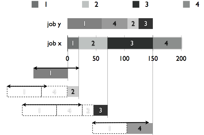
(a) Sample problem.

Machine	$1$	$2$	$3$	$4$
${t_{i}},{t_{j}}$	${t_{1}},{t_{5}}$	${t_{2}},{t_{7}}$	${t_{3}},{t_{8}}$	${t_{4}},{t_{6}}$
${p_{i}}$	20	50	80	50
${h_{i}}$	0	20	70	150
${p_{j}}$	60	20	25	45
${h_{j}}$	0	105	125	60
$-f(j,i)$	-60	-105	-80	45
$f(i,j)$	20	-35	25	140

(b) Values of ${p}$, ${h}$ and $f{}$.

Figure 1: Computation of conflict intervals.

In Figure 1a we illustrate two jobs ${J_{x}}=\{{t_{1}},{t_{2}},{t_{3}},{t_{4}}\}$ and ${J_{y}}=\{{t_{5}},{t_{6}},{t_{7}},{t_{8}}\}$. The number and shades of grey stand for the machine required by each task. The length of the tasks are respectively $\{20,50,80,50\}$ for ${J_{x}}$ and $\{60,45,20,25\}$ for ${J_{y}}$. In Figure 1b we give, for each machine, the pair of conflicting tasks, their durations and the corresponding forbidden intervals.

For each machine ${M_{k}}$, let ${t_{i}}$ be the task of ${J_{x}}$ and ${t_{j}}$ the task of ${J_{y}}$ that are both processed on machine ${M_{k}}$. Following the reasoning used in Model 4, we have a conflict interval (represented by black arrows in Figure 1a) for each pair of tasks sharing the same machine: ${J_{y}}\not\in~{}]{J_{x}}-f(j,i),{J_{x}}+f(i,j)[$. In the example the forbidden intervals for ${J_{y}}$ are therefore: $]{J_{x}}-60,{J_{x}}+20[\ldots]{J_{x}}-105,{J_{x}}-35[\ldots]{J_{x}}-80,{J_{x}}+25[\ldots]{J_{x}}+45,{J_{x}}+140[$. However, these intervals can be merged, yielding larger (maximal) forbidden intervals, in which case we have: ${J_{y}}\not\in]{J_{x}}-105,{J_{x}}+25[~{}\wedge~{}{J_{y}}\not\in]{J_{x}}+45,{J_{x}}+140[$.

Data: ${J_{x}}=\{{t_{x_{1}}},\ldots,{t_{x_{m}}}\},~{}{J_{y}}=\{{t_{y_{1}}},\ldots,{t_{y_{m}}}\},{\cal M}$ $I_{in}\leftarrow[]$;

foreach ${t_{x_{i}}}\in{J_{x}},{t_{y_{j}}}\in{J_{y}}$ such that ${\cal M}({t_{x_{i}}})={\cal M}({t_{y_{j}}})$ do

  $I_{in}\leftarrow I_{in}$ extended with $[(-f(j,i),+1),(f(i,j),-1)]$;

 sort $I_{in}$ by increasing first element;

$I_{out}\leftarrow[]$;  $open\leftarrow 0$;

while not-empty$(I)$ do

  $(a,z)\leftarrow$ remove first element from $I_{in}$;

if $open=0$ then append $a$ to $I_{out}$;

$open\leftarrow open+z$;

if $open=0$ then append $a$ to $I_{out}$;

 return $I_{out}$;

Algorithm 2 get-F-intervals.

Given two jobs ${J_{x}}$ and ${J_{y}}$, Algorithm 2 computes all maximal forbidden intervals efficiently (in $O(m\log m)$ steps). First, we build a list of pairs whose first element is an end point of a conflict interval, and second element is either $+1$ if it is the start, and $-1$ otherwise. Then these pairs are sorted by increasing first element. Now we can scan these pairs and count, thanks to the second element, how many intervals are simultaneously open. When we go from $0$ to $1$ open intervals, this marks the start of a maximal forbidden interval, and conversely the end when we go from $1$ to $0$ open intervals. The list $I_{out}$ has $2k$ elements, and the $2i+1^{th}$ and $2i+2^{th}$ elements are read as the start and end of a forbidden interval.

Given this set of forbidden intervals, we can represent the conflicts between ${J_{x}}$ and ${J_{y}}$ with the following set of Boolean variables and disjunctive constraints:

$${b_{xy}}^{105,25}=\left\{\begin{array}[]{cl}0\Leftrightarrow{J_{y}}+105\leq{J_{x}}\\ 1\Leftrightarrow{J_{x}}+25\leq{J_{y}}\end{array}\right.$$

$${b_{xy}}^{45,140}=\left\{\begin{array}[]{cl}0\Leftrightarrow{J_{y}}-45\leq{J_{x}}\\ 1\Leftrightarrow{J_{x}}+140\leq{J_{y}}\end{array}\right.$$

In the previous encoding we would have needed $4$ Boolean variables and as many disjunctive constraints (one for each pair of tasks sharing a machine). We believe, however, that the main benefit is not the reduction in size of the encoding. Rather, it is the tighter correlation between the model and the real structure of the problem which helps the heuristic to make good choices.

model 5 NW-JSP

$$minimise~{}C_{max}~{}~{}{\rm subject~{}to:}$$

$$C_{max}\geq{J_{x}}+\sum_{{t_{i}}\in{J_{x}}}{p_{i}} \qquad\forall{J_{x}}\in{\cal J}$$ (4.7)

$${b_{ij}}^{a,b}=\left\{\begin{array}[]{cl}0\Leftrightarrow{J_{y}}-a\leq{J_{x}}\\ 1\Leftrightarrow{J_{x}}+b\leq{J_{y}}\end{array}\right. \qquad\forall{J_{x}}\neq{J_{y}}\in{\cal J},[a,b]\in\texttt{get-F-intervals}({J_{x}},{J_{y}},{\cal M})$$ (4.10)

5 Experimental Evaluation

The full experimental results, with statistics for each instance, as well as benchmarks and source code are online: http://homepages.laas.fr/ehebrard/jsp-experiment.html.

5.1 Job Shop with Earliness/Tardiness Objective

The best complete methods for handling these types of problem are the CP/LP hybrid of Beck and Refalo [4] and the MIP approaches of Danna et al. [9], and Danna and Perron [8], while more recently Kebel and Hanzalek proposed a pure CP approach [14]. Danna and Perron also proposed an incomplete approach based on large neighborhood search [8].

Our experiments were run on an Intel Xeon 2.66GHz machine with 12GB of ram on Fedora 9. Each algorithm run on a problem had an overall time limit of 3600s, and there were 10 runs per instance. We report our results in terms of the best and worst run. We tested our method on two benchmarks which have been widely studied in the literature. The comparison experimental results are taken from [9] and [8], where all experiments were performed on a 1.5 GHz Pentium IV system running Linux. For the first benchmark, these algorithms had a time limit of 20 minutes per instance, while for the second benchmark the algorithms had a time limit of 2 hours.

The comparison methods are as follows:

• MIP: Default CPLEX in [9], run using a modified version of ILOG CPLEX 8.1

• CP: A pure constraint programming approach introduced by Beck and Refalo in [4], run using ILOG Scheduler 5.3 and ILOG Solver 5.3

• CRS-ALL: A CP/LP hybrid approach proposed by Beck and Refalo in [4], run using ILOG CPLEX 8.1, ILOG Hybrid 1.3.1, ILOG Scheduler 5.3 and ILOG Solver 5.3

• uLNS: An unstructured large neighborhood search MIP method proposed by Danna and Peron in [8], run using a modified version of ILOG CPLEX 8.1

• sLNS: A structured large neighborhood search CP/LP method proposed by Danna and Peron in [8], run using ILOG Scheduler 5.3, ILOG Solver 5.3 and ILOG CPLEX 8.1

The first benchmark consists of 9 sets of problems generated by Beck and Refalo [4] using the random JSP generator of Watson et al. [26]. For instance size ${\cal J}$x${\cal M}$, there were three sets of ten JSPs of size 10x10, 15x10 and 20x10 generated. The second benchmark is taken from the genetic algorithms (GA) literature and was proposed by Morton and Pentico [18]. There are 12 instances, with problem size ranging from 10x3 to 50x8. Jobs in these problems do have release dates. Furthermore earliness and tardiness costs of a job are equal.

We present results on the randomly generated ETJSPs in Table 1 in terms of number of problems solved to optimality and sum of the upper bounds, for each algorithm. Here, the column “Best” for our method means the number of problems solved to optimality on at least one of the ten runs on the instance, while the column “Worst” refers to the number of problems solved to optimality on all ten runs. We also report the mean cpu time in seconds for our method.

Table 1: ET-JSP - Random Problems, Number Proven Optimal and Upper Bound Sum

$lf$	MIP		CP		uLNS		sLNS	CRS-All		Model 2
										Best		Worst		Avg.
	opt.	$\sum$ub	opt.	$\sum$ub	opt.	$\sum$ub	$\sum$ub	opt.	$\sum$ub	opt.	$\sum$ub	opt.	$\sum$ub	Time (s)
1.0	0	654,290	0	1,060,634	0	156,001	52,307	7	885,546	10	30,735	8	38,416	2534.86
1.3	14	26,930	6	1,248,618	30	8,397	8,397	30	8,397	30	8,397	30	8,397	0.36
1.5	27	7,891	6	1,672,511	30	6,964	6,964	30	6,964	30	6,964	30	6,964	0.18
Notes: Comparison results taken from [9], except uLNS, taken from [8].
Figures in bold are the best result over all methods.

We first consider the number of problems solved to optimality (columns “Opt.”). While there is little difference in the performance of our method and that of uLNS and CRS-ALL on the looser instances (looseness factor of 1.3 and 1.5), we see that our method is able to close three of the 23 open problems in the set with looseness factor 1.0. An obvious reason for this improvement with our method would be the difference in time limits and quality of machines. However, analysis of the results reveals that of the 68 problems solved to optimality on every run of our method, only 8 took longer than one second on average, and only one took longer than one minute (averaging 156s). Furthermore, uLNS only solved two problems to optimality when the time limit was increased to two hours [8]. Clearly our method is extremely efficient at proving optimality on these problems.

The previous results suggest that CRS-ALL is much better than uLNS on these problems. However, as was shown by Danna et al. [9], this may not be the case when the algorithms are compared based on the sum of the upper bounds found over the 30 “hard” instances (i.e. with looseness factor 1.0). In order to assess whether there was a similar deterioration in the performance of our method as for CRS-ALL on the problems where optimality was not proven, we report this data in the columns “$\sum$ub” of Table 1.

We find, on the contrary, that the performance of our approach is even more impressive when algorithms are compared using this metric. The two large neighborhood search methods found the best upper bounds of the comparison algorithms with sLNS the most efficient by a factor of 2 over uLNS. However, there are a couple of points that should be noted here. Firstly sLNS is an incomplete method so cannot prove optimality, and secondly the sum of the worst upper bounds found by our method was still significantly better than that found by sLNS. Indeed, there was very little variation in performance for our method across runs, with an average difference of 256 between the best and worst upper bounds found.

Danna and Perron also provided the sum of the best upper bounds found on the hard instances over all methods they studied [8], which was 36,459. This further underlines the quality of the performance of our method on these problems. Finally, we investigated the hypothesis that the different time limit and machines used for experiments could explain these results. We compared the upper bounds found by our method after the dichotomic search phase, where the maximum runtime of this phase over all runs per instance was 339s. The upper bound sums over the hard instances were 32,299 and 49,808 for best and worst respectively, which refutes this hypothesis.

Table 2: ET-JSP - GA Problems, Normalized upper bounds

Instance	Size	MIP	CP	uLNS	sLNS	CRS-All	GA	Model 2
							Best	Best	Worst
jb1	10x3	0.191*	0.474	0.191*	0.191	0.191*	0.474	0.191*	0.191*
jb2	10x3	0.137*	0.746	0.137*	0.137	0.531	0.499	0.137*	0.137*
jb4	10x5	0.568*	0.570	0.568*	0.568	0.568*	0.619	0.568*	0.568*
jb9	15x3	0.333*	0.355	0.333*	0.333	1.216	0.369	0.333*	0.333*
jb11	15x5	0.233	0.365	0.213*	0.213	0.213*	0.262	0.221	0.235
jb12	15x5	0.190*	0.239	0.190*	0.190	0.190*	0.246	0.190*	0.190*
	GMR	1.015	1.774	1	1	1.555	1.610	1.006	1.017
ljb1	30x3	0.215*	0.847	0.215*	0.215	0.295	0.279	0.215	0.221
ljb2	30x3	0.622	1.268	0.508	0.508	1.364	0.598	0.590	0.728
ljb7	50x5	0.317	0.614	0.123	0.110	0.951	0.246	0.166	0.256
ljb9	50x5	1.373	1.737	1.270	1.015	2.571	0.739	1.157	1.513
ljb10	50x8	0.820	1.569	0.558	0.525	1.779	0.512	0.499	0.637
ljb12	50x8	1.025	1.368	0.488	0.605	1.601	0.399	0.537	0.623
	GMR	1.943	3.233	1.213	1.170	4.098	1.220	1.299	1.686
Overall GMR		1.329	2.434	1.084	1.068	2.305	1.408	1.118	1.256
Comparison results taken from [9]. Figures in bold indicate best upper bound
found over the different algorithms. “*” indicates optimality was proven by the algorithm.

Table 2 provides results on the second of the benchmarks (taken from the GA literature). Following the convention of previous work on these problems [23][4][9], we report the cost normalized by the weighted sum of the job processing times. We include the best results found by the GA algorithms as presented by Vázquez and Whitley [23]. We also provide an aggregated view of the results of each algorithm using the geometric mean ratio (GMR), which is the geometric mean of the ratio between the normalized upper bound found by the algorithm and the best known normalized upper bound, across a set of instances.

The performance of our method was less impressive for these problems, solving two fewer problems to optimality than uLNS, and achieving a worse GMR than either of the large neighborhood search methods. However, we remind the reader that all comparison methods had a 2 hour time limit on these instances, except the GA approaches for which the time limit was not reported. We further note that we find an improved solution for one instance (ljb10) and outperform all methods other than uLNS and sLNS.

5.2 Job Shop Scheduling Problem with positive Time Lags

These experiments were run using the same settings as in Section 5.1. However, because of the large number of instances and algorithms, we used only 5 random runs per instance.

There are relatively few results reported for benchmarks with positive maximum time lag constraints, as most publications focus on the “no wait” case. Caumond et al. introduced a genetic algorithm [7]. Then, Artigues et al. introduced a Branch & Bound procedure that allowed them to find lower bounds of good quality [1]. Therefore, in order to get a better idea of the efficiency of our approach, we adapted a model written by Chris Beck for Ilog Scheduler (version 6.3) to problems featuring time lag constraints. This model was used to showcase the SGMPCS algorithm [3]. We used the following two strategies: In the first, the next pair of tasks to schedule is chosen following the Texture heuristic/goal predefined in Ilog Scheduler and restarts following the Luby sequence [16] are performed, this was one of the default strategies used as a reference point in [3]. In the second, branching decisions are selected with the same “goal”, however the previous best solution is used to decide wich branch should be explored first, and geometric restarts [25] are performed, instead of the Luby sequence. In other words, this is SGMPCS with a singleton elite solution. We denote the first method Texture-Luby and the second method Texture-Geom+Guided. These two methods were run on the same hardware with the same time limit and number of random runs as our method. Finally, we report results for our approach without the greedy initialization heuristic (Algorithm 1) in order to evaluate its importance.

We used the benchmarks generated by Caumond et al. in [7] by adding maximal time lag constraints to the Lawrence JSP instances of the OR-library. Given a job shop instance N, and two parameters $x$ and $y$, a new instance N_$x$_$y$ is produced. For each job all maximal time lags are given the value $ym$, where $m$ is the average processing time over tasks of this job. The first parameter $x$ corresponds to minimal time lags and will always be 0 in this paper.

Table 3: TL-JSP - Comparison with related work (Time & Upper bound).

Instance	[AHL]		[CLT]		Model 3
	time (s)	$C_{max}$	time (s)	$C_{max}$	time (s)	$C_{max}$
la06_0_10	707.00	927	0.00	926	0.03	926
la06_0_1	524.00	1391	1839.00	1086	70.60	926
la07_0_10	518.00	1123	25.00	890	3600.00	890
la07_0_1	754.00	1065	1914.00	1032	3600.00	896
la08_0_10	260.00	863	2.00	863	0.07	863
la08_0_1	587.00	1052	1833.00	1048	615.80	892
average	558.33	1070	935.50	974	1314.41	898
$PRD$		18.88		8.32		0.00

Due to space limitations, we present most of our results in terms of each solver’s average percentage relative deviation (PRD) given by the following formula: $PRD=((C_{Alg}-C_{Ref})/C_{Ref})*100$, where $C_{Alg}$ is the best makespan found by the algorithm and $C_{Ref}$ is the best upper bound among all considered algorithms. In Table 3, we first report a comparison with the genetic algorithm described in [7], denoted [CLT] and the adhoc Branch & Bound algorithm introduced in [1], denoted [AHL]. We used only instances for which results were reported in both papers, and where the time lags were strictly positive, hence the relatively small data set. Despite that, and despite the difference in hardware and time limit, it is quite clear that our approach outperforms both the complete and heuristic methods on these benchmarks.

Table 4: TL-JSP - Comparison with Ilog Scheduler (Proofs of optimality & Upper bound PRD).

Instance Sets	Texture				Model 3
	Luby		Geom+Guided		no init.		init. heuristic
	Opt.	$PRD$	Opt.	$PRD$	Opt.	$PRD$	Opt.	$PRD$
la[1,40]_0_0	0.12	25.37	0.12	16.15	0.37	10.42	0.35	0.06
la[1,40]_0_0.25	0.20	22.98	0.25	12.01	0.37	3.46	0.40	0.00
la[1,40]_0_0.5	0.22	19.47	0.25	5.17	0.37	2.62	0.42	0.00
la[1,40]_0_1	0.35	15.76	0.42	1.18	0.40	17.43	0.45	0.47
la[1,40]_0_2	0.67	7.35	0.75	0.13	0.67	74.16	0.70	0.37
la[1,40]_0_3	0.75	3.47	0.92	0.00	0.75	95.91	0.77	0.29
la[1,40]_0_10	0.95	0.10	0.97	0.00	0.92	0.04	0.92	0.05

Next, in Table 4, we report results on all modified Lawrence instances for both Ilog Scheduler models, and the two version of Model 3, with and without the greedy initialization heuristic. Since there are 280 instances in total, the results are aggregated by the level of tightness of the time lag constraints. For each set, we give the ratio of instances that were solved to optimality in at least one of the five runs in the first column, as well as the mean PRD in the second column.

First, we notice the great impact of the new initialization heuristic on our method. Without it, the Ilog Scheduler model was more efficient for instances with $y=1$, and the overall results are extremely poor for larger values of $y$. However, the mean results are deceptive. Without initialization, Model 3 can be very efficient, although in a few cases no solution at all can be found. Indeed, relaxing the makespan does not necessarily makes the problem easy for this model. The weight of these bad cases in the mean value can be important, hence the poor PRD. On the other hand, we can see that the Ilog Scheduler model is more robust to this phenomenon: a non-trivial upper bound is found in every case. It is therefore likely that the impact of the initialization heuristic will not be as important on the Ilog model as on Model 3.

We also notice that solution guidance and geometric restarts greatly improve Ilog Scheduler’s performance. Interestingly, we observe that our approach is best when the time lag constraints are tight. On the other hand, Scheduler is slightly more efficient on instances with loose time lag constraints and in particular proves optimality more often on these instances. However, whereas our method always finds near-optimal solutions (the worst mean PRD is 0.47 for instances with $y=1$), both scheduler models find relatively poor upper bounds for small values of $y$.

5.3 Job Shop Scheduling Problem with no wait constraints

For the no-wait job shop problem, the best methods are a tabu search method by Schuster (TS [20]) and a hybrid constructive/tabu search algorithm introduced by Bożejko and Makuchowski in 2009 (HTS [6]). We also report the results of a Branch & Bound procedure introduced by Mascis and Pacciarelli [17]. This algorithm was run on a Pentium II 350 MHz.

Table 5: NW-JSP - Comparison with related work (Upper bound PRD).

Instance	Mascis et al.	Schuster	Bożejko et al.		Model 4		Model 5
	B&B	TS	HTS	HTS+	$tdom$+$bw$	$tdom/tw$	$tdom$+$bw$	$tdom/tw$
la[1-10]	0.00	4.43	1.77	1.77	0.00	0.00	0.00	0.00
la[11-20]	31.66	7.93	3.49	0.95	0.14	0.10	0.00	0.31
la[21-30]	61.09	10.43	7.25	0.08	1.16	0.57	0.25	0.84
la[31-40]	73.73	10.95	8.33	0.15	4.42	1.77	2.68	1.36
abz[5-9]	47.04	9.01	5.95	0.78	2.47	1.14	1.13	1.20
orb[1-10]	0.00	2.42	0.77	0.77	0.00	0.00	0.00	0.00
swv[1-5]	60.85	3.94	3.67	0.00	2.54	0.77	0.00	0.43
swv[6-10]	57.82	4.99	4.19	0.00	4.78	1.71	0.44	1.00
swv[11-15]	70.98	0.68	2.48	0.60	19.50	6.53	17.54	5.18
swv[16-20]	76.81	5.71	3.98	0.00	10.92	68.94	4.47	3.17
yn[1-4]	72.74	12.40	8.85	0.32	5.60	5.75	2.37	2.88
overall	44.72	6.51	4.36	0.52	3.53	5.50	1.97	1.13

For the no-wait class we used the same data sets as Schuster [20] and Bożejko et al. [6] where null time lags are added to instances of the OR-library. We report the best results of each paper in terms of average PRD. It should be noted that for HTS, the authors reported two sets of results. The former were run with a time limit based on the runtimes reported in [20] and varying from 0.25 seconds for the easiest instances to $2360$ seconds for the hardest. The latter (in italic font, and referred to as HTS+ in Table 5) were run “without limit of computation time”. We use bold face to mark the best result amongst methods that had time limits, i.e. excluding HTS+. We ran two variable ordering heuristics for our method. First, the heuristics used for ET-JSP and TL-JSP, where the Boolean variable minimizing the value of $(max({t_{i}})+max({t_{j}})-min({t_{i}})-min({t_{j}})+2)/(w({t_{i}})+w({t_{j}}))$ is chosen first, denoted $tdom/tw$. Second, we used another heuristic, denoted $tdom$+$bw$ that selects the next Boolean variable to branch on solely according to the tasks’ domain sizes $(max({t_{i}})+max({t_{j}})-min({t_{i}})-min({t_{j}})+2)$, and break ties with the Boolean variable’s own weight $w({b_{ij}})$.

Table 6: NW-JSP - New best upper bounds and optimality proofs.

Instance		Schuster	Bożejko		Model 4		Model 5
	BKS	TS	HTS	HTS+	$tdom$+$bw$	$tdom/tw$	$tdom$+$bw$	$tdom/tw$
la11_0_0	2821	1737	1704	1621	1622	1619	1619*	1621
la13_0_0	2650	1701	1696	1580	1582	1590	1580*	1580
la14_0_0	2662	1771	1722	1610	1578	1578	1578*	1612
la15_0_0	2765	1808	1747	1686	1692	1679	1671*	1691
la26_0_0	4268	2664	2738	2506	2624	2511	2488	2540
la28_0_0	4478	2886	2741	2552	2640	2605	2546	2569
la30_0_0	4097	2939	2791	2452	2452	2452	2452*	2508
la34_0_0	6380	3957	3936	3659	3914	3693	3817	3657
la39_0_0	4295	2804	2725	2687	2660	2660	2660*	2660
swv01	3824	2396	2424	2318	2344	2343	2318*	2333
swv02	3800	2492	2484	2417	2440	2418	2417*	2417
swv05	3836	2482	2489	2333	2433	2333	2333*	2333
yn2	4025	2705	2647	2370	2486	2603	2427	2353
yn4	4109	2705	2630	2513	2532	2573	2499	2582

In Table 6 we report the results on no-wait instances for which we obtained new upper bounds (5 instances) or new proofs of optimality (9 instances), thanks to the model introduced here.

6 Conclusions

We have shown that the simple constraint programming approach introduced in [13] can be successfully adapted to handle the objective of minimizing the sum of earliness/tardiness costs. These problems have traditionally proven troublesome for CP approaches because of the weak propagation of the sum objective [8].

Then we introduced a new heuristic to find good initial solutions for job shop problems with maximal time lag constraints. The resulting method greatly improves over state of the art algorithms for this problem. However, as opposed to the other aspects of the method (adaptive variable heuristic, solution guided branching, restarts with nogood storage) this new initialization heuristic is dedicated to job shop problems with time lag constraints.

Finally, we showed that domain-specific information can also be used to improve our model for no-wait job shop scheduling problems, allowing us to provide several improved upper bounds and prove optimality in many cases.

References

- [1] C. Artigues, M-J. Huguet, and P. Lopez. Generalized Disjunctive Constraint Propagation for Solving the Job Shop Problem with Time Lags. EAAI, 24(2):220 – 231, 2011.
- [2] P. Baptiste, M. Flamini, and F. Sourd. Lagrangian Bounds for Just-in-Time Job-shop Scheduling. Computers & OR, 35(3):906–915, 2008.
- [3] J. C. Beck. Solution-Guided Multi-Point Constructive Search for Job Shop Scheduling. JAIR, 29:49–77, 2007.
- [4] J. C. Beck and P. Refalo. A Hybrid Approach to Scheduling with Earliness and Tardiness Costs. Annals OR, 118(1-4):49–71, 2003.
- [5] F. Boussemart, F. Hemery, C. Lecoutre, and L. Sais. Boosting Systematic Search by Weighting Constraints. In ECAI, pages 482–486, 2004.
- [6] W. Bozejko and M. Makuchowski. A Fast Hybrid Tabu Search Algorithm for the No-wait Job Shop Problem. Computers & Industrial Engineering, 56(4):1502–1509, 2009.
- [7] A. Caumond, P. Lacomme, and N. Tchernev. A Memetic Algorithm for the Job-shop with Time-lags. Computers & OR, 35(7):2331–2356, 2008.
- [8] E. Danna and L. Perron. Structured vs. unstructured large neighborhood search: A case study on job-shop scheduling problems with earliness and tardiness costs. Technical report, ILOG, 2003.
- [9] E. Danna, E. Rothberg, and C. Le Pape. Integrating Mixed Integer Programming and Local Search: A Case Study on Job-Shop Scheduling Problems. In CPAIOR, 2003.
- [10] T. Feydy and P. J. Stuckey. Lazy Clause Generation Reengineered. In CP, pages 352–366, 2009.
- [11] D. Grimes. A Study of Adaptive Restarting Strategies for Solving Constraint Satisfaction Problems. In AICS, 2008.
- [12] D. Grimes and E. Hebrard. Job Shop Scheduling with Setup Times and Maximal Time-Lags: A Simple Constraint Programming Approach. In CPAIOR, pages 147–161, 2010.
- [13] D. Grimes, E. Hebrard, and A. Malapert. Closing the Open Shop: Contradicting Conventional Wisdom. In CP’09, pages 400–408, 2009.
- [14] J. Kelbel and Z. Hanzálek. Solving production scheduling with earliness/tardiness penalties by constraint programming. J. Intell. Manuf., 2010.
- [15] C. Lecoutre, L. Sais, S. Tabary, and V. Vidal. Nogood Recording from Restarts. In IJCAI, pages 131–136, 2007.
- [16] M. Luby, A. Sinclair, and D. Zuckerman. Optimal Speedup of Las Vegas Algorithms. In ISTCS, pages 128–133, 1993.
- [17] A. Mascis and D. Pacciarelli. Job-shop Scheduling with Blocking and No-wait Constraints. EJOR, 143(3):498–517, 2002.
- [18] T. E. Morton and D. W. Pentico. Heuristic Scheduling Systems. John Wiley and Sons, 1993.
- [19] C. Rajendran. A No-Wait Flowshop Scheduling Heuristic to Minimize Makespan. The Journal of the Operational Research Society, 45(4):472–478, 1994.
- [20] C. J. Schuster. No-wait Job Shop Scheduling: Tabu Search and Complexity of Problems. Math Meth Oper Res, 63:473–491, 2006.
- [21] A. Schutt, T. Feydy, P. J. Stuckey, and M. Wallace. Why Cumulative Decomposition Is Not as Bad as It Sounds. In CP’09, pages 746–761, 2009.
- [22] N. Tamura, A. Taga, S. Kitagawa, and M. Banbara. Compiling Finite Linear CSP into SAT. In CP, pages 590–603, 2006.
- [23] M. Vázquez and L. D. Whitley. A comparison of genetic algorithms for the dynamic job shop scheduling problem. In GECCO, pages 1011–, 2000.
- [24] P. Vilím. Filtering Algorithms for the Unary Resource Constraint. Archives of Control Sciences, 18(2), 2008.
- [25] T. Walsh. Search in a Small World. In IJCAI, pages 1172–1177, 1999.
- [26] J-P. Watson, L. Barbulescu, A. E. Howe, and L. D. Whitley. Algorithm performance and problem structure for flow-shop scheduling. In AAAI, pages 688–695, 1999.
- [27] D. A. Wismer. Solution of the Flowshop-Scheduling Problem with No Intermediate Queues. Operations Research, 20(3):689–697, 1972.