An Approximation of the
Universal Intelligence Measure

Abstract

The Universal Intelligence Measure is a recently proposed formal definition of intelligence. It is mathematically specified, extremely general, and captures the essence of many informal definitions of intelligence. It is based on Hutter’s Universal Artificial Intelligence theory, an extension of Ray Solomonoff’s pioneering work on universal induction. Since the Universal Intelligence Measure is only asymptotically computable, building a practical intelligence test from it is not straightforward. This paper studies the practical issues involved in developing a real-world UIM-based performance metric. Based on our investigation, we develop a prototype implementation which we use to evaluate a number of different artificial agents.

1 Introduction

A fundamental problem in strong artificial intelligence is the lack of a clear and precise definition of intelligence itself. This makes it difficult to study the theoretical or empirical aspects of broadly intelligent machines. Of course there is the well-known Turing Test (Turing,, 1950), however this paradoxically seems to be more about dodging the difficult problem of explicitly defining intelligence than addressing the real issue. We believe that until we have a more precise definition of intelligence, the quest for generally intelligent machines will lack reliable techniques for measuring progress.

One recent attempt at an explicit definition of intelligence is the Universal Intelligence Measure (Legg and Hutter,, 2007). This is a mathematical, non-anthropocentric definition of intelligence that draws on a range of proposed informal definitions of intelligence, algorithmic information theory (Li and Vitányi,, 2008), Solomonoff’s model of universal inductive inference (Solomonoff,, 1964, 1978), and Hutter’s AIXI theory of universal artificial intelligence (Hutter,, 2001, 2005). This paper conducts a preliminary investigation into the potential for this particular measure of intelligence to serve as a practical metric for evaluating real-world agent implementations.

2 Background

We now briefly describe the recently introduced notion of a Universal Intelligence Test, the Universal Intelligence Measure and the practical issues that arise when attempting to evaluate the performance of broadly intelligent agents.

2.1 Universal Intelligence Tests

Hernández-Orallo and Dowe, (2010) introduce the notion of a Universal Intelligence Test, a test designed to be able to quantitatively assess the performance of artificial, robotic, terrestrial or even extra-terrestrial life, without introducing an anthropocentric bias. Related discussion on the motivation behind such tests is given by Dowe and Hajek, (1998); Hernández-Orallo, (2000); Schaul et al., (2011). With respect to our goal of wanting to build more powerful artificial agents, we strongly support the introduction of such general purpose tests. Having a suite of such tests, with each emphasizing different, measurable aspects of intelligence, would clearly help the community build more powerful and robust general agents. This paper introduces our own such test, which works by approximating the Universal Intelligence Measure.

2.2 Universal Intelligence Measure

After surveying some 70 informal definitions of intelligence proposed by various psychologists and artificial intelligence researchers, Legg and Hutter (2007) argue that the informal definition:

“intelligence measures an agent’s ability to achieve goals in a wide range of environments”,

broadly captures many important properties associated with intelligence. To formalise this intuition, they used reinforcement learning (Sutton and Barto,, 1998), a general framework for goal achieving agents in unknown environments. In this setting, cycles of interaction occur between the agent and the environment. At each cycle, the agent sends an action to the environment, that then responds with an observation and (scalar) reward. The agent’s goal is to choose its actions, based on its previous observations and rewards, so as to maximise the rewards it receives over time. With a little imagination, it is not hard to see that practically any problem can be expressed in this framework, from playing a game of chess to writing an award-winning novel.

In their setup, both the agent and environment are expressed as conditional probability measures over interaction sequences. To formalise a ‘wide range of environments’, the set of all Turing computable environments is used, with the technical constraint that the sum of returned rewards is finitely bounded. Finally, the agent’s performance over different environments is then aggregated into a single result. To encourage agents to apply Occam’s Razor, as advocated by Legg and Hutter, (2007), each environment is weighted according to its complexity, with simpler environments being weighted more heavily. This is elegantly achieved by using the algorithmic prior distribution (Li and Vitányi,, 2008). The universal intelligence of an agent $\pi$ can then be defined as,

$$\Upsilon(\pi)\,:=\,\sum_{\mu\in E}2^{-K(\mu)}V_{\mu}^{\pi}$$ (1)

where $\mu$ is an environment from the set $E$ of all computable reward bounded environments, $K(\cdot)$ is the Kolmogorov complexity, and $V_{\mu}^{\pi}:=\mathbb{E}(\sum_{i=1}^{\infty}R_{i})$ is the expected sum of future rewards when agent $\pi$ interacts with environment $\mu$.

This theoretical measure of intelligence has a range of desirable properties. For example, the most intelligent agent under this measure is Hutter’s AIXI, a universal agent that converges to optimal performance in any environment where this is possible for a general agent (Hutter,, 2005). At the other end of the scale, it can be shown that the Universal Intelligence Measure sensibly orders the performance of simple adaptive agents. Thus, the measure spans an extremely wide range of capabilities, from the simplest reactive agents up to universally optimal agents. Unlike the pass or fail Turing test, universal intelligence is a continuous measure of performance and so it is more informative of incremental progress. Furthermore, the measure is non-anthropocentric as it is based on the fundamentals of mathematics and computation rather than human imitation.

The major downside is that the Universal Intelligence Measure is only a theoretical definition, and is not suitable for evaluating real-world agents directly.

3 Algorithmic Intelligence Quotient

The aim of the Universal Intelligence Measure was to define intelligence in the most general, precise and succinct way possible. While these goals were achieved, this came at the price of asymptotic computability. In this section we will show how a practical measure of machine intelligence can be defined via approximating this notion. While we will endeavor to retain the spirit of the Universal Intelligence Measure, the emphasis of this section will be on practicality rather than theoretical purity. We will call our metric the Algorithmic Intelligence Quotient or AIQ for short.

3.1 Environment sampling

One way to define an Occam’s Razor prior is to use the Universal Distribution (Solomonoff,, 1964). The universal prior probability, with respect to a reference machine $\mathcal{U}$, of a sequence beginning with a finite string of bits $x$ is defined as

$$M_{\mathcal{U}}(x)\,:=\!\sum_{p:\mathcal{U}(p)=x*}\!\!2^{-\ell(p)},$$

where $\mathcal{U}(p)=x*$ means that the universal Turing machine $\mathcal{U}$ computes an output sequence that begins with $x$ when it runs program $p,$ and $\ell(p)$ is the length of $p$ in bits. As the Kolmogorov complexity of $x*$ is the length of the shortest program for $x*$, by definition, it follows that the largest term in $M$ is given by $2^{-K(x*)}$. Thus, the set of all sequences that begin with a low complexity string will have a high prior probability under $M$, in accordance with Occam’s Razor. The difference now is that the lengths of all programs that generate strings beginning with $x$ are used to define the prior, not just the shortest program.

The advantage of switching to this related distribution is that it is much easier to sample from. As the probability of sampling a program $p$ by uniformly sampling consecutive bits is $2^{-\ell(p)}$, to sample a sequence from $M$ we just randomly sample a program $p$ and run it on $\mathcal{U}$. This method of sampling has been used to create the test data sequences that make up the Generic Compression Benchmark (Mahoney,, 2008). Here we will use this technique to sample environments for the Universal Intelligence Measure. More precisely, having defined a prefix-free universal Turing machine ${\mathcal{U}}$, we generate a finite sample of $N$ programs $S:=p_{1},p_{2},\ldots,p_{N}$ by uniformly generating bits until we reach the end of each program. This is not a set as the same program can be sampled many times. The estimate of agent $\pi$’s universal intelligence is then,

$$\hat{\Upsilon}(\pi)\,:=\,\frac{1}{N}\sum_{i=1}^{N}\hat{V}_{p_{i}}^{\pi},$$

where we have replaced the expectation $V_{\mu}^{\pi}$ with $\hat{V}_{p_{i}}^{\pi}$ which is defined to be the empirical total reward returned from a single trial of environment $\mathcal{U}(p_{i})$ interacting with agent $\pi$. Since we are sampling the space of programs that define environments, rather than the space of environments directly, multiple programs can define the same environment. Notice that the weighting by $2^{-\ell(p_{i})}$ is no longer needed as the probability of a program being sampled decreases by $\frac{1}{2}$ for every additional bit. The natural idea of performing a Monte Carlo sample over environments is also used by Hernández-Orallo and Dowe, (2010) and Schaul et al., (2011) in their related work.

3.2 Environment simulation

We need to be able to run each sampled program on our reference machine $\mathcal{U}$. A technical problem we face is that some programs will not halt, and due to the infamous halting problem, we know there is no process that can always determine when this is the case. The extent of this problem can be reduced by choosing a reference machine where non-halting programs are relatively unlikely, or one which aids the detection of many non-halting programs. Even so, we would still have non-halting problems to deal with.

From a practical perspective there is not much difference between a program that does not halt and one that simply runs for too long: in both cases the program needs to be discarded. To determine if this is the case, we first run the program on the reference machine. If the program exceeds our computation limit in any cycle, the program is discarded. In the future, more powerful hardware will allow us to increase this limit to obtain more accurate AIQ estimates.

3.3 Temporal preference

In the Universal Intelligence Measure, the total reward that an environment can return is upper bounded by one. Because all computable environments that respect this constraint are considered, in effect the Universal Intelligence Measure considers all computable distributions of rewards. Theoretically this is elegant, but practically we have no way of knowing if a program will respect the bound.

A more practical alternative is geometric discounting (Sutton and Barto,, 1998) where we allow the environment to generate any reward in any cycle so long as the reward belongs to a fixed bounded interval. Rewards are then scaled by a factor that decreases geometrically with each interaction cycle. Under such a scheme the reward sum is bounded and thus we can bound the remaining reward left in a trial. For example, we can terminate each trial once the possible remaining reward drops below a certain value.

While this is elegant, it is not very computationally efficient when we are interested in learning over longer time frames. This is since the later cycles, where the agent has most likely learnt the most, are the most heavily discounted. Thus, we will focus here on undiscounted, bounded rewards over fixed length trials.

3.4 Reference machine selection

When looking at converting the Universal Intelligence Measure into a concrete test of intelligence, a major issue is the choice of a suitable reference machine. Unfortunately, there is no such thing as a canonical universal Turing machine, and the choice that we make can have a significant impact on the test results. Very powerful agents such as AIXI will achieve high universal intelligence no matter what reference machine we choose, assuming we allow agents to train from samples prior to taking the test, as suggested in Legg and Hutter, (2007). For more limited agents however, the choice of reference machine is important. Indeed, in the worst case it can cause serious problems (Hibbard,, 2009). When used with typical modern reinforcement learning algorithms and a fairly natural reference machine, we expect the performance of the test to lie between these two extremes. That is, we expect that the reference machine will be important, but perhaps not so important that we will be unable to construct a useful test of machine intelligence. Providing some empirical insight into this is one of the main aims of this paper.

Before choosing a reference machine, it is worth considering, in broad terms, the effect that different reference machines will have on the intelligence measure. For example, if the reference machine is like the Lisp programming language, environments that can be compactly described using lists will be more probable. This would more heavily weight these environments in the measure, and thus if we were trying to increase the universal intelligence of an agent with respect to this particular reference machine, we would progress most rapidly if we focused our effort on our agent’s ability to deal with this class of environments. On the other hand, with a more Prolog like reference machine, environments with a logical rule structure would be more important. More generally, with a simple reference machine, learning to deal with small mathematical, abstract and logical problems would be emphasised as these environments would be the ones computed by small programs. These tests would be more like the sequence prediction and logical puzzle problems that appear in some IQ tests.

What about very complex reference machines? This would permit all kinds of strange machines, potentially causing the most likely environments to have bizarre structures. As we would like our agents to be effective in dealing with problems in the real world, if we do use a complex reference machine, it seems the best choice would be to use a machine that closely resembles the structure of the real world. Thus, the Universal Intelligence Measure would become a simulated version of reality, where the probability of encountering any given challenge would reflect its real world likelihood. Between these extremes, a moderately complex reference machine might include three dimensional space and elementary physics. While complex reference machines allow the intelligence measure to be better calibrated to the real world, they are far more difficult to develop. Thus, at least for our first set of tests, we focus on using a very simple reference machine.

3.5 BF reference machine

One important property of a reference machine is that it should be easy to sample from. The easiest languages are ones where all programs are syntactically valid and there is a unique end of program symbol. One language with this feature is Urban Müller’s BF language. It has just 8 symbols, listed in Table 1 along with their C equivalents, where we have used C stdin and stdout at the input and output tapes, and p is a pointer to the work tape.

BF		C
>	move pointer right	p++;
<	move pointer left	p--;
+	increment cell	*p++;
-	decrement cell	*p--;
.	write output	putchar(*p);
,	read input	*p = getchar();
[	if cell is non-zero, start loop	while(*p) {
]	return to start of loop	}

Table 1: Standard BF program symbols along with their C equivalents.

To convert BF for use as a reference machine the agent’s action information is placed on input tape cells, then the program is run, and the reward and observation information is collected from the output tape. Reward is the first symbol on the output tape and is normalised to the range -100 to +100. The following symbol is the observation. All symbols on the input, output and work tapes are integers, with a modulo applied to deal with under/over flow conditions. As discussed in Section 3.2, we set a time limit for the environment’s computation in each interaction cycle, here 1000 computation steps. To encourage programs to terminate, we interpret any attempt to write excess reward and observation cells as a signal to halt computation for that interaction cycle. As a result about 90% of programs do not exceed the computation limit and halt with output for each cycle.

As we do not wish our environments to always be deterministic, we have added to BF the instruction % which writes a random symbol to the current work tape cell. Furthermore, we also place a history of previous agent actions on the input tape. This solves the problem of what to do when a program reads too many input symbols, and it also makes it easier for the environment to compute functions of the agent’s past actions. Finally, after randomly sampling a program we remove any pointless code, such as “+-”, “><” and “[]”. This produces faster and more compact programs, and discards the most common type of pointless infinite loop. We also discard programs that do not contain any instructions to either read from the input or write to the output.

Finally, the first bit of the program indicates whether the reward values are negated or not. By randomly setting this bit, randomly acting agents have an AIQ of zero, a natural baseline suggested by Hernández-Orallo and Dowe, (2010).

3.6 Variance Reduction Techniques for AIQ Estimation

Obtaining an accurate estimate of an agent’s AIQ using simple Monte-Carlo sampling can be time consuming. This is due to the relatively slow rate at which the standard error decays as the number of samples increases, along with the fact that for many agents, simulating even a single episode is quite demanding. To help our implementation provide statistically significant results within reasonable time constraints, we applied a number of techniques that significantly reduced the variance of our AIQ estimates.

The first technique was to simply exploit the parallel nature of Monte Carlo sampling so that the test could be run on multiple cores. On present day hardware, this can easily lead to a 10x performance improvement over a single core implementation.

The second technique was to use stratified sampling. It works as follows: first, the sample space $\Omega$ is partitioned into $k$ mutually exclusive sets $\Omega_{1},\Omega_{2},\dots,\Omega_{k}$ such that $\bigcup_{i=1}^{k}\Omega_{i}=\Omega$. Each $\Omega_{i}$ is called a stratum. The total probability mass $\Pr[X\in\Omega_{i}]$ associated with each of the $k$ strata needs to be known in advance. Given a sample $(X_{1},X_{2},\dots,X_{n})$, the stratified estimate $\hat{X}_{ss}$ is given by,

$$\hat{X}_{ss}:=\sum_{i=1}^{k}\Pr[X\in\Omega_{i}]\left(\frac{1}{n_{i}}\sum_{j=1}^{n}X_{j}\mathbb{I}[X_{j}\in\Omega_{i}]\right)$$

where $n_{k}:=\sum_{i=1}^{n}\mathbb{I}[X_{i}\in\Omega_{k}]$. It can be interpreted as a convex combination of $k$ simple Monte Carlo estimates, and is easily shown to be unbiased. For a fixed sample size, the optimal way to allocate samples is in proportion to the standard deviation of each stratum, weighted by the stratum’s probability mass. More precisely, if $f_{X}(x)$ is the density function of $X$ and $f_{k}(x)\mathbb{\propto I}[x\in\Omega_{k}]f_{X}(x)$ is the density function associated with the random variable $Y_{k}$ associated with stratum $k$, the optimal allocation ratio is achieved when $n_{k}\propto\sqrt{\mathrm{Var}[Y_{k}]}\Pr[X\in\Omega_{k}]$. To do this we must estimate $\mathrm{Var}[Y_{k}]$ during sampling and adapt which strata we are drawing samples from accordingly. Intuitively, the algorithm is identifying those parts of the sample space which have the most variance and are of the most significance to the final result, and concentrating the sampling effort in these regions. There are various algorithms for adaptive stratified sampling, however we have chosen the method developed by Étoré and Jourdain, (2010) as they have derived the confidence intervals for the estimate of the mean, a feature we will use when reporting our results. In AIQ, we stratified on a combination of simple properties of each environment program, including the length and the presence of particular patterns of BF symbols. This particular technique gave roughly a 4x performance increase.

Another variance reduction technique we used was common random numbers. Rather than estimating the AIQ of two agents $\pi$ and $\pi^{\prime}$ from independent samples from the environment distribution, we instead estimate the difference,

$$\hat{\Delta}(\pi,\pi^{\prime}):=\hat{\Upsilon}(\pi^{\prime})-\hat{\Upsilon}(\pi)$$

using a single set of program samples. This technique is particularly important when an agent designer is deciding whether or not to accept a new version of the agent. Intuitively, common random numbers reduces the chance of one agent performing better due to being evaluated on an easier sample. More precisely,

$$\mathrm{Var}[\hat{\Delta}(\pi,\pi^{\prime})]=\mathrm{Var}[\hat{\Upsilon}(\pi^{\prime})]+\mathrm{Var}[\hat{\Upsilon}(\pi)]-2\mathrm{Cov}[\hat{\Upsilon}(\pi^{\prime}),\hat{\Upsilon}(\pi)].$$

If independent samples were used for $\hat{\Upsilon}(\pi^{\prime})$ and $\hat{\Upsilon}(\pi)$ the covariance would vanish. However, since we are using a single sample and have assumed that the AIQs of $\pi$ and $\pi^{\prime}$ are positively correlated (which makes sense if $\pi^{\prime}$ is an incremental improvement over $\pi$), $\mathrm{Cov}[\hat{\Upsilon}(\pi^{\prime}),\hat{\Upsilon}(\pi)]$ is positive and thus $\mathrm{Var}[\hat{\Delta}(\pi,\pi^{\prime})]$ is reduced.

The final variance reduction technique we used was antithetic variates. The intuition is quite straightforward: instead of using one sample, use two samples in such a way that the resultant estimators for the first and second sample are negatively correlated. These can then be combined to balance each other out, thus reducing the total variance. More formally, if $\hat{Y}_{1}$and $\hat{Y}_{2}$ are two unbiased estimates of a quantity of interest, then $\hat{{X}}=\tfrac{1}{2}[\hat{Y}_{1}+\hat{Y}_{2}]$ is also an unbiased estimator, with

$$\mathrm{Var}(\hat{{X})}=\tfrac{1}{4}\left[{\mathrm{Var}(\hat{Y}_{1})}+\mathrm{Var}(\hat{Y}_{2})+2\mathrm{Cov}(\hat{Y}_{1},\hat{Y}_{2})\right].$$

Thus if the two estimates are negatively correlated, $\mathrm{Var}(\hat{{X})}$ is reduced. A common way to achieve this is to sample in pairs, with each element of the pair directly opposing the other in some sense. In our AIQ implementation, since the first bit of each program specifies whether or not to negate the rewards, applying antithetic variates was trivial: we simply ran each program twice, once with the first bit off, once with the first bit on. This lead to a performance improvement that varied based on the agent being tested. With the exception of the Random agent (where there was a massive negative correlation), the performance improvements were typically smaller than a factor of 1.5x.

4 Empirical results

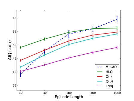
Figure 1: Estimated AIQ scores of agents as a function of episode length.

We implemented AIQ with the variance reduction techniques previously described, along with the extended BF reference machine. Our code is open source and available for download at www.vetta.org/aiq. It should run on any platform containing Python and the Scipy library. We have also implemented a number of reinforcement learning agents to test AIQ with. The simplest agent is called Random, which makes uniformly random actions. A slightly more complex agent is Freq, that computes the average reward associated with each action, ignoring observation information. It chooses the best action in each cycle except for a fixed fraction of the time when it tries a random action. We have implemented the $Q(\lambda)$ algorithm (Watkins,, 1989), which subsumes the simpler $Q(0)$ algorithm as a special case, and also $HLQ(\lambda)$ which is similar except that it automatically adapts its learning rate (Hutter and Legg,, 2007). Finally, we have created a wrapper for MC-AIXI (Veness et al.,, 2010, 2011), a more advanced reinforcement learning agent that can be viewed as an approximation to Hutter’s AIXI.

4.1 Comparison of artificial agents

For our first set of tests we took the BF reference machine and set the number of symbols on the tape to 5. We then tested all our agents without discounting on a range of different episode lengths. With the exception of MC-AIXI, which is significantly more computationally expensive, we performed 10,000 samples in each test. As expected, the AIQ of the Random agent was zero. For the other agents we ran parameter sweeps to find the best performing settings. These results appear in Figure 1, with the error bars representing approximate 95% confidence intervals.

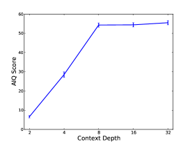
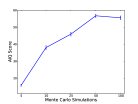
Figure 2: Estimated AIQ of MC-AIXI as the context depth and search effort is varied.

For 100k length episodes the agents’ AIQ scores appear in the order that we would expect: Random (not shown), Freq, $Q(0)$, $Q(\lambda)$, $HLQ(\lambda)$ and MC-AIXI. As the episode lengths decrease, the agent’s have less learning time in each trial and thus their scores decline. Except for MC-AIXI, the relative ranking of the agents remained the same. It seems MC-AIXI’s complex world model is relatively slow to learn but ultimately the most powerful. Our initial attempts at modifying MC-AIXI to be similarly high scoring on shorter runs failed. Longer tests may be needed in order to determine whether some of the more complicated agents have reached their maximal AIQ.

Similar tests to the above were performed with 2, 10 and 20 symbol tapes. The results were qualitatively the same, but with larger action and observation spaces the learning times increased for all agents. We also increased the number of cells used to represent the observations, usually set to 1, which had the same effect. We then tried reversing the order of the observation and the reward on the tape, which lead to results that were qualitatively the same. We experimented with discounting, and the results were consistent with the undiscounted results using shorter episodes lengths. We also increased the computation limit per cycle and did not see any measurable effect. Thus our initial findings were that the results seemed relatively robust to minor modifications of the reference machine.

4.2 Measuring Agent Scalability

The MC-AIXI agent has a parameter that sets the context depth of its prediction algorithm, in effect controlling the maximal size of the world model that it can learn. It also has a parameter that specifies the number of Monte Carlo simulations it generates, in effect controlling the amount of effort that it puts into planning for each interaction cycle. These two parameters allow us to vary the power of the MC-AIXI agent along two fundamentally different dimensions. We did this with a 5 symbol BF reference machine, as before, and with 50k length episodes. The results of these tests appear in Figure 2. While increasing the agent’s search effort consistently increased its AIQ score, the results for the context depth appear to have plateaued at a depth of 8, though with the present error bars it is impossible to tell for sure. This warrants future investigation. For example, it may be the case that larger context depths help only if the episode length is longer than 50,000.

4.3 Environment Distribution

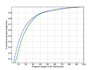
Figure 3: A comparison of the BF program lengths in the environment distribution compared to the environments chosen by the adaptive sampler. The dashed blue line shows the cumulative proportion of BF environments satisfying a given maximum program length. The solid green line shows the cumulative proportion of BF environments sampled by our variance reduction enhanced adaptive sampling procedure.

We next ran some tests to help characterise our environment sampling procedure.

Our first test involved generating $2\times 10^{5}$ legal BF environment programs satisfying the criteria listed in Section 3.5. For example, programs that ran too long or didn’t have both a read and a write instruction were discarded. The dashed blue line in Figure 3 shows the resultant empirical cumulative distribution of program lengths across the space of BF environments. Although the number of programs at any given length decays exponentially, this result shows that a significant amount of the total probability mass is still allocated to relatively complex environments with description lengths of 20 symbols or more.

Our next test involved inspecting the distribution of programs sampled by our adaptive sampler when evaluating the HLQ agent. This is shown by the green line on Figure 3. This shows that the adaptive sampler reduces the proportion of programs of length 10 or less from almost 40% to 20%. On the other hand, from length $20$ to $40$ the green line climbs more quickly then the blue one. Thus we see that the adaptive sampler has moved the sampling effort away from programs shorter than 20 symbols, and focused its effort on the $20$ to $40$ symbol range.

We also visually inspected a variety of generated environments. While it is true that extremely short programs, for example those of less than 5 symbols, do not generate very interesting environments, we found that by the time we got to programs of length 30, many environments (at least to our eyes) seemed quite incomprehensible.

5 Related Work and Discussion

Hernandez-orallo and Minaya-collado, (1998) developed a related test, called the C-test, that is also based on a very simple reference machine. Like BF it uses a symbolic alphabet with an end wrap around. Unlike BF, which is a tape based machine, the C-test uses a register machine with just three symbol registers. This means that the state space for programs is much smaller than in BF. Another key difference is that the C-test considers generated sequences of symbols, rather than fully interactive environments. In our view, this makes it not a complete test of intelligence. For example, the important problem of exploration does not feature in a non-interactive setting. Extending the C-test reference machine to be interactive would likely be straightforward: simply add instructions to read and write to input and output tapes, the same way BF does. It would be interesting to see how AIQ behaves when using such a reference machine.

A different approach is used by Insa-Cabrera et al., 2011b ; Insa-Cabrera et al., 2011a . Here an interactive reinforcement learning setting is considered, however the space of environments is no longer sampled from a Turing complete reference machine. Instead a small MDP is used (3, 6 and 9 states) with uniformly random transitions. Which state is punishing or rewarding follows a fixed random path through this state space. To measure the complexity of environments, the gzip compression algorithm is applied to a description of the environment. While this makes the test tractable, in our view it does so in a way that deviates significantly from the Universal Intelligence Measure that we are attempting to approximate with AIQ. Interestingly, in their setting human performance was not better than the simple tabular Q-learning algorithm. We suspect that this is because their environments have a simple random pattern structure, something that algorithms are well suited for compared to humans.

Another important difference in our work is that we have directly sampled from program space. This is analogous to the conventional construction of the Solomonoff prior, which samples random bit sequences and treats them as programs. With this approach all programs that compute some environment count towards the environment’s effective complexity, not just the shortest, though the shortest clearly has the largest impact. This makes AIQ very efficient in practice since we can just run sampled programs directly, avoiding the need to have to compute complexity values through techniques such as brute force program search. For example, to compute the complexity of a 15 symbol program, the C-test required the execution of over 2 trillion programs. For longer programs, such as many that we have used in our experiments, this would be completely intractable. One disadvantage of our approach, however, is that we never know the complexity of any given environment; instead we know just the length of one particular program that computes it.

6 Conclusion

We have taken the theoretical model of Legg and Hutter, (2007) and converted it into a practical test for machine intelligence. To do this we have randomly sampled programs from a simple universal Turing machine, drawing inspiration at points from Hernández-Orallo and Dowe, (2010), and the related work in Hernández-Orallo, (2010). In all of our tests the AIQ scores behaved sensibly, with agents expected to be more intelligent having higher AIQ. Naturally, no empirical test can confirm that a test of intelligence is indeed “correct”, rather it can only confirm that the theoretical model behaves as expected when suitably approximated, and that no insurmountable difficulties arise when attempting this. We believe that our present efforts have been successful in this regard, but more work is clearly required.

Perhaps the most worrying potential problem with the Universal Intelligence Measure is its dependence on the choice of reference machine, as highlighted by Hibbard, (2009). While we accept that problematic reference machines exist, it was our belief that if we chose a fairly simple and natural reference machine, the resulting intelligence test would behave sensibly. While we have only provided one data point to support this claim here, the fact that it was the first and only reference machine that we tried gives us hope that it is not overly special. Furthermore, we found that the results were qualitatively the same for a range of minor modifications to the BF reference machine. Obviously, further reference machines will need to be implemented and tested to gain a greater understanding of these issues.

Acknowledgements

This research was supported by Swiss National Science Foundation grant number PBTIP2-133701.

References

- Dowe and Hajek, (1998) Dowe, D. L. and Hajek, A. R. (1998). A non-behavioural, computational extension to the Turing Test. In Intl. Conf. on Computational Intelligence & multimedia applications (ICCIMA’98), Gippsland, Australia, pages 101–106.
- Étoré and Jourdain, (2010) Étoré, P. and Jourdain, B. (2010). Adaptive optimal allocation in stratified sampling methods. Methodology and Computing in Applied Probability, 12(3):335–360.
- Hernández-Orallo, (2000) Hernández-Orallo, J. (2000). Beyond the Turing Test. J. Logic, Language & Information, 9(4):447–466.
- Hernández-Orallo, (2010) Hernández-Orallo, J. (2010). A (hopefully) unbiased universal environment class for measuring intelligence of biological and artificial systems. In Proc. of the Third Conference on Artificial General Intelligence, Lugano.