Search for the signal of monotop production at the early LHC

Abstract

We investigate the potential of the early LHC to discover the signal of monotops, which can be decay products of some resonances in models such as R-parity violating SUSY or SU(5), etc. We show how to constrain the parameter space of the models by the present data of $Z$ boson hadronic decay branching ratio, $K^{0}-\overline{K^{0}}$ mixing and dijet productions at the LHC. Then, we study the various cuts imposed on the events, reconstructed from the hadronic final states, to suppress backgrounds and increase the significance in detail. And we find that in the hadronic mode the information from the missing transverse energy and reconstructed resonance mass distributions can be used to specify the masses of the resonance and the missing particle. Finally, we study the sensitivities to the parameters at the LHC with $\sqrt{s}$=7 TeV and an integrated luminosity of $1~{}{\rm fb}^{-1}$ in detail. Our results show that the early LHC may detect this signal at 5$\sigma$ level for some regions of the parameter space allowed by the current data.

I Introduction

The main tasks of the Large Hadron Collider (LHC) are to answer the fundamental questions in particle physics: whether the Higgs boson exist or not. And are there new physics beyond standard model (SM) such as supersymmetry (SUSY), extra dimension, etc, at the TeV scale? Generally, it is believed that top quark may have strong connections with new physics due to its large mass close to the scale of electroweak symmetry breaking. The production topologies of top quark pair production with or without missing transverse energy ${E\!\!\!/}_{T}$ have been extensively investigated Alvarez et al. (2011); Haisch and Westhoff (2011); Berger et al. (2011); Cao et al. (2011); Degrande et al. (2011); Battaglia and Servant (2010); Cao et al. (2010); Alwall et al. (2010); Han et al. (2009); Barger et al. (2008). However the topology of a single top and ${E\!\!\!/}_{T}$, which is so-called monotop Andrea et al. (2011), has only been discussed recently Kamenik and Zupan (2011); Dong et al. (2011). This signal is absent in the SM and occur in models such as R-parity violating SUSY and SU(5) as decay products of resonance production of some particles. In R-parity violating SUSY Barbier et al. (2005), a stop can be produced by the fusion of two down-type anti-quarks through the Yukawa-like trilinear interaction $\lambda_{ijk}^{{}^{\prime\prime}}U_{i}^{c}D_{j}^{c}D_{k}^{c}$, where $U_{i},D_{i}$ are left-handed chiral superfields and the superscript $c$ denotes the charge conjugate, and then the stop decays into a top quark and a neutralino which could not be detected at the collider. In the SU(5) model Barr (1982), the gauge bosons $X$, in one case, can transform quarks to anti-quarks assigned to the 10 representation; in the other case, they couple to quarks and leptons in the 5 representation. As a result, they can be resonantly produced at hadron colliders and decay into a top and a neutrino. Therefore, any discovery of such signal imply new physics, and may help us to explore the fundamental questions mentioned above.

In this work, we propose the general model-independent renormalizable effective Lagrangian with $\rm SU(3)_{c}\times SU(2)_{L}\times U(1)_{Y}$ gauge symmetry

$$\mathcal{L}=\lambda_{S}^{ij}\epsilon^{\alpha\beta\gamma}\phi_{\alpha}\bar{d}_{i\beta R}^{c}d_{j\gamma R}+a_{S}^{i}\phi_{\alpha}\bar{u}^{\alpha}_{iR}\chi+\lambda_{V}^{ij}\epsilon^{\alpha\beta\gamma}X_{\mu,\alpha}\bar{d}_{i\beta R}^{c}\gamma^{\mu}d_{j\gamma R}+a_{V}^{i}X_{\mu,\alpha}\bar{u}^{\alpha}_{iR}\gamma^{\mu}\chi+h.c.,$$ (1)

where there is a summation over the generation indices $i,j=1,2,3,$ and $\rm SU(3)_{c}$ gauge indices $\alpha,\beta,\gamma=1,2,3$. The superscript $c$ denotes charge conjugation. The Dirac field $\chi$ is a singlet under the SM gauge group and manifest itself as missing energy at colliders. The scalar and vector fields $\phi$ and $X_{\mu}$ are color triplet resonances that can appear in some models, which obtain their masses at high energy scales. This Lagrangian could further be generalized, such as shown in Ref. Andrea et al. (2011), although it may not be gauge invariant any more. The free parameters in Eq. (1) are masses of the resonances and missing particle, i.e., $m_{\phi},m_{X}$ and $m_{\chi}$, and couplings $\lambda_{S,V}^{ij}$ and $a_{S,V}^{i}$, which should be constrained by current precise data, and will be investigated carefully in this paper. Here, we only consider the case of scalar resonance field $\phi$, and the case of vector resonance field $X_{\mu}$ will be studied elsewhere.

The scenario of monotop production has been explored in Ref. Andrea et al. (2011), where they only consider the mode of top hadronic decay. In the case of resonant monotop production, they assume the branching fraction of $\phi\to t\chi$ equal to one and neglect the decay channel of $\phi\to\bar{d}\bar{s}$, which would lead to an overestimation of the signal. But we will take into account all decay channels of the resonance, which turns out to be very important for estimating the sensitivity to detect the signal at the LHC. Moreover, we also discuss the mode of semileptonic decay of top quark besides hadronic decay. Although the cross section of the backgrounds for semileptonic decay mode are very large, the discovery of the signal in this mode is still possible once appropriate cuts are imposed.

This paper is organized as follows. In Sec. II, we consider the constraints on the free parameters from $Z$ hadronic decay branching ratio, $K^{0}-\overline{K^{0}}$ mixing and dijet experiments at the LHC. In Sec. III, we investigate the signal and backgrounds of monotop production in detail and then analyze the discovery potential at the early LHC. A conclusion is given in Sec. IV.

II Experiment Constraints

The experiments have set constraints on the stop production and decay, the signal of which is similar to the monotop, in R-parity violating SUSY so far. For example, the H1 Aktas et al. (2004) and ZEUS Chekanov et al. (2007) collaborations at HERA have analyzed the process of stop resonantly produced by electron-quark fusion and followed either by a direct R-parity-violating decay, or by the gauge boson decay. The process of stop pair production and decaying into dielectron plus dijet at the Tevatron is also discussed Chakrabarti et al. (2003). However, these results can not be converted to constraints on the parameters in our case. Here the relevant experiments, we are concerned with, are $Z$ hadronic decay branching ratio, $K^{0}-\overline{K^{0}}$ mixing and dijet production at the LHC.

II.1 $Z$ hadronic decay branching ratio

The effective Lagrangian in Eq. (1) may contribute to the branching fraction of $Z$ boson hadronic decay as shown in Fig. 1. From the precise measurement of branching fraction of $Z$ boson hadronic decay, the relevant bands on R-parity violating SUSY parameters have been investigated in Ref. Bhattacharyya et al. (1995). Since the quarks in the effective Lagrangian are right-handed, the couplings of right-handed quarks with $Z$ boson are modified, and thus affect the branching fraction of $Z$ boson hadronic decay.

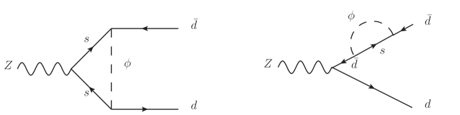
Figure 1: Feynman diagrams for hadronic $Z$ boson decay induced by the field $\phi$.

The tree-level amplitude of $Z$ boson decaying into a pair of quarks in the SM can be parameterized as

$$\mathcal{M}_{\mu}=g_{Z}\bar{q}(p_{1})\gamma^{\mu}(a_{L}^{q}P_{L}+a_{R}^{q}P_{R})q(p_{2}),$$ (2)

where

$$g_{Z} = \frac{e}{s_{W}c_{W}},$$

$$a_{L}^{q} = t_{3}^{q}-Q_{q}s_{W}^{2},$$

$$a_{R}^{q} = -Q_{q}s_{W}^{2}.$$ (3)

After calculating the Feynman diagrams in Fig. 1, we find that the coefficient $a_{R}^{q}$ is adjusted by multiplying a factor

$$1+\Delta_{f}=1+\frac{\lambda_{f}^{2}}{8\pi^{2}}g(a),$$ (4)

where $a=M_{Z}^{2}/m_{\phi}^{2}$ and $f=1,2,3$ correspond to $Z$ boson decaying into $d\bar{d}$, $s\bar{s}$ and $b\bar{b}$, respectively. And $\lambda_{f}$ are defined as

$$\lambda_{1}^{2} = 4[(\lambda_{S}^{12})^{2}+(\lambda_{S}^{13})^{2}],$$ (5)

$$\lambda_{2}^{2} = 4[(\lambda_{S}^{12})^{2}+(\lambda_{S}^{23})^{2}],$$ (6)

$$\lambda_{3}^{2} = 4[(\lambda_{S}^{13})^{2}+(\lambda_{S}^{23})^{2}],$$ (7)

where we have used the fact that $\lambda_{S}^{ij}=-\lambda_{S}^{ji}$ due to the antisymmetry of the $\epsilon^{\alpha\beta\gamma}$ couplings in Eq. (1). The explicit form of function $g(a)$ is

$$g(a) = \frac{(a-4)a-2\log(a)((a-2)a+2\log(a+1))-4\text{Li}_{2}(-a)}{4a^{2}}.$$ (8)

The ultraviolet poles of the triangle and self-energy diagrams have canceled each other, and we obtain a finite result. In this calculation, all the masses of quarks are neglected. Eq. (8) seems divergent if $a$ vanishes due to the denominator $a^{2}$. But actually we expand this result around $a=0$, and get the asymptotic form

$$g(a)=\left(\frac{1}{9}-\frac{\log(a)}{3}\right)a+\left(\frac{\log(a)}{4}-\frac{1}{16}\right)a^{2}+\left(\frac{1}{25}-\frac{\log(a)}{5}\right)a^{3}+O\left(a^{4}\right),$$ (9)

which vanishes obviously when taking the limit $a\to 0$. This feature guarantees the decouple of the heavy particle $\phi$ in the large $m_{\phi}$ limit.

There are two observables which can be affected by the change of coefficient $a_{R}^{q}$. One is $R_{l}\equiv\Gamma_{h}/\Gamma_{l}$, where $\Gamma_{h,l}$ are the widths of $Z$ boson decaying into hadrons and leptons, respectively. The correction to $R_{l}$ is

$$\delta R_{l} = \frac{\Gamma_{h}-\Gamma_{h}^{SM}}{\Gamma_{l}^{SM}}$$ (10)

$$= \frac{2(\Delta_{1}\Gamma_{dR}^{SM}+\Delta_{2}\Gamma_{sR}^{SM}+\Delta_{3}\Gamma_{bR}^{SM})}{\Gamma_{l}^{SM}},$$

where $\Gamma_{qR}^{SM},q=d,s,b$ denote the widths of $Z$ boson decaying into only right-handed $q$ quarks in the SM. The other is $R_{b}\equiv\Gamma_{b}/\Gamma_{h}$, where $\Gamma_{b}$ is the width into $b\bar{b}$. Explicitly, we can write $R_{b}$ as

$$R_{b} = \frac{\Gamma_{b}}{\Gamma_{h}}$$ (11)

$$= \frac{1+2\Delta_{3}\frac{\Gamma_{bR}^{SM}}{\Gamma_{b}^{SM}}}{1+2\Delta_{1}\frac{\Gamma_{dR}^{SM}}{\Gamma_{h}^{SM}}+2\Delta_{2}\frac{\Gamma_{sR}^{SM}}{\Gamma_{h}^{SM}}+2\Delta_{3}\frac{\Gamma_{bR}^{SM}}{\Gamma_{h}^{SM}}}\frac{\Gamma_{b}^{SM}}{\Gamma_{h}^{SM}}.$$

Thus, the correction to $R_{b}$ is given by

$$\delta R_{b} \approx 2\left[\Delta_{3}\frac{\Gamma_{bR}^{SM}}{\Gamma_{b}^{SM}}\left(1-\frac{\Gamma_{b}^{SM}}{\Gamma_{h}^{SM}}\right)-\Delta_{1}\frac{\Gamma_{dR}^{SM}}{\Gamma_{d}^{SM}}\frac{\Gamma_{d}^{SM}}{\Gamma_{h}^{SM}}-\Delta_{2}\frac{\Gamma_{sR}^{SM}}{\Gamma_{s}^{SM}}\frac{\Gamma_{s}^{SM}}{\Gamma_{h}^{SM}}\right]R_{b}^{SM}.$$ (12)

The experiments give $R_{e}=20.804\pm 0.050$, $R_{\mu}=20.785\pm 0.033$, $R_{\tau}=20.764\pm 0.045$ and $R_{b}=0.2163\pm 0.0007$, respectively, while the SM predictions are $R_{e}^{SM}=R_{\mu}^{SM}=20.735$, $R_{\tau}^{SM}=20.780$ and $R_{b}^{SM}=0.2158$ Nakamura et al. (2010). The requirement that the corrected $R_{e,\mu,\tau,b}$ are in the $1\sigma$ range around the experimental central values imposes constraints as follows,

$$(\lambda_{1}^{2}+\lambda_{2}^{2}+\lambda_{3}^{2})\frac{g(a)}{4\pi^{2}}<0.829,0.578,0.202{~{}~{}~{}\rm for}~{}~{}R_{e},R_{\mu},R_{\tau},{\rm respectively},$$ (13)

and

$$-0.0289<[0.78\lambda_{3}^{2}-0.22(\lambda_{1}^{2}+\lambda_{2}^{2})]\frac{g(a)}{4\pi^{2}}<0.173{~{}~{}~{}\rm for}~{}~{}R_{b}.$$ (14)

We show the allowed region by $R_{\tau}$ and $R_{b}$ for $\lambda_{S}$ as a function of $m_{\phi}$ in Fig. 2. The solid and dashed lines are the upper limits given by $R_{\tau}$ for the cases $\lambda_{S}^{12}=\lambda_{S}^{13}=\lambda_{S}^{23}=\lambda_{S}$ and $\lambda_{S}^{12}=\lambda_{S},\lambda_{S}^{13}=\lambda_{S}^{23}=0$, respectively. The dotted line is the upper limit given by $R_{b}$ for $\lambda_{S}^{12}=\lambda_{S},\lambda_{S}^{13}=\lambda_{S}^{23}=0$. From Fig. 2 we can see that this constraint on the parameter is not very stringent. This is due to the fact that only right-handed couplings are corrected, and the widths of $Z$ boson decaying into right-handed quarks are much less than into left-handed quarks.

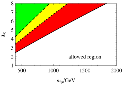
Figure 2: The allowed region by $Z$ boson hadronic decay branching fraction as a function of $m_{\phi}$. The solid and dashed lines are the upper limits given by $R_{\tau}$ for the cases $\lambda_{S}^{12}=\lambda_{S}^{13}=\lambda_{S}^{23}=\lambda_{S}$ and $\lambda_{S}^{12}=\lambda_{S},\lambda_{S}^{13}=\lambda_{S}^{23}=0$, respectively. The dotted line is the upper limit given by $R_{b}$ for $\lambda_{S}^{12}=\lambda_{S},\lambda_{S}^{13}=\lambda_{S}^{23}=0$.

II.2 $K^{0}-\overline{K^{0}}$ mixing

Now we consider the constraint from $K^{0}-\overline{K^{0}}$ mixing. The typical Feynman diagram for $K^{0}-\overline{K^{0}}$ mixing is shown in Fig. 3.

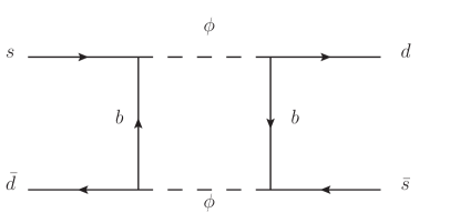
Figure 3: Representative Feynman diagram for $K^{0}-\overline{K^{0}}$ mixing.

After straightforward calculations, we can obtain

$$\mathcal{H}_{eff}^{\Delta S=2}=CQ,$$ (15)

where $Q$ is the operator $\bar{d}_{R}^{\alpha}\gamma^{\mu}s_{R}^{\alpha}\bar{d}_{R}^{\beta}\gamma^{\mu}s_{R}^{\beta}$, and $C$ is its Wilson coefficient,

$$C=\frac{(\lambda_{S}^{13}-\lambda_{S}^{31})^{2}(\lambda_{S}^{23}-\lambda_{S}^{32})^{2}}{32\pi^{2}}\left[\frac{m_{\phi}^{4}-m_{b}^{4}-2m_{b}^{2}m_{\phi}^{2}\ln\frac{m_{\phi}^{2}}{m_{b}^{2}}}{(m_{\phi}^{2}-m_{b}^{2})^{3}}\right]b(\mu),$$ (16)

where

$$b(\mu)=(\alpha_{s}(\mu))^{-2/9}\left(1+\frac{307}{162}\frac{\alpha_{s}(\mu)}{4\pi}\right)$$ (17)

contains the renormalization scale dependence Herrlich and Nierste (1995). We have compared this result with that in Refs. de Carlos and White (1997); Slavich (2001) and find our result is consistent with their results. Then, the $K_{L}-K_{S}$ mass difference $\Delta m_{K}$ is given by Ciuchini et al. (1998)

$$\Delta m_{K}=2{\rm Re}\langle K^{0}|\mathcal{H}_{eff}^{\Delta S=2}|\overline{K^{0}}\rangle=2C{\rm Re}\langle K^{0}|Q|\overline{K^{0}}\rangle.$$ (18)

The matrix element $\langle K^{0}|Q|\overline{K^{0}}\rangle$ can be parameterized as

$$\langle K^{0}|Q|\overline{K^{0}}\rangle=\frac{1}{3}m_{K}f_{K}^{2}B_{K}(\mu)$$ (19)

where $m_{K}$ is the mass of $K^{0}$ (497.6 MeV), $f_{K}$ is kaon decay constant (160 MeV), and $B_{K}(\mu)$ is related to the renormalization group invariant parameter $\hat{B}_{K}$ by

$$\hat{B}_{K}=B_{K}(\mu)b(\mu).$$ (20)

In our numerical analysis we will use the following result Buras (1998):

$$\hat{B}_{K}=0.75\pm 0.15.$$ (21)

On the other hand, the SM contribution to $\Delta m_{K}$ is

$$\Delta m^{SM}_{K}=\frac{G_{F}^{2}}{6\pi^{2}}f_{K}^{2}\hat{B}_{K}m_{K}M_{W}^{2}{\rm Re}[\lambda_{c}^{\ast 2}\eta_{1}S_{0}(x_{c})+\lambda_{t}^{\ast 2}\eta_{2}S_{0}(x_{t})+2\lambda_{c}^{\ast}\lambda_{t}^{\ast}\eta_{3}S_{0}(x_{c},x_{t})]$$ (22)

where $\lambda_{i}=V_{is}^{\ast}V_{is}$, and $V_{ij}$ are the CKM matrix elements. The functions $S_{0}$ are given by

$$S_{0}(x_{t}) = \frac{4x_{t}-11x_{t}^{2}+x_{t}^{3}}{4(1-x_{t})^{2}}-\frac{3x_{t}^{3}\ln x_{t}}{2(1-x_{t})^{3}},$$

$$S_{0}(x_{c}) = x_{c},$$

$$S_{0}(x_{c},x_{t}) = x_{c}\left[\ln\frac{x_{t}}{x_{c}}-\frac{3x_{t}}{4(1-x_{t})}-\frac{3x_{t}^{2}\ln x_{t}}{4(1-x_{t})^{2}}\right]$$ (23)

with $x_{i}=m_{i}^{2}/M_{W}^{2}$. The next-to-leading values of $\eta_{i}$ are given as follows Buras et al. (1990); Herrlich and Nierste (1994); Urban et al. (1998):

$$\eta_{1}=1.38\pm 0.20,\quad\eta_{2}=0.57\pm 0.01,\quad\eta_{3}=0.47\pm 0.04.$$ (24)

We require that the contribution to $\Delta m_{K}$, including the SM and new physics result, is not larger than the experimental value $\Delta m_{K}^{\rm exp}=(3.483\pm 0.006)\times 10^{-15}~{}\rm GeV$ Nakamura et al. (2010) within $1\sigma$ level, assuming the CPT conservation. In Fig. 4, we show the allowed region for $\lambda_{S}$ as a function of $m_{\phi}$ for $\lambda_{S}^{13}=\lambda_{S}^{23}=\lambda_{S}$. From Fig. 4 we find that the constraint on $\lambda_{S}$ is very stringent, generally less than 0.06. Furthermore, these couplings involves the third generation quarks, the parton distribution functions (PDFs) of which are small compared with those of the first two generations. Therefore, we choose $\lambda_{S}^{13}=\lambda_{S}^{23}=0$, for simplicity, in the following discussion.

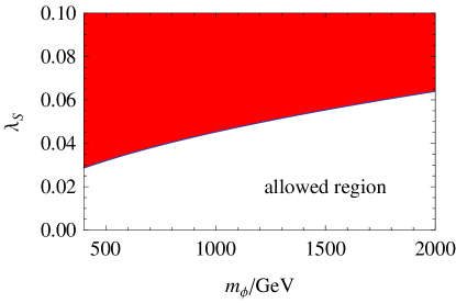
Figure 4: The allowed region of $\lambda_{S}$ ($=\lambda_{S}^{13}=\lambda_{S}^{23}$) by $K^{0}-\overline{K^{0}}$ mixing as a function of $m_{\phi}$.

II.3 Dijet production at the LHC

The dijet experiments at the LHC have set upper limits on the product of cross section ($\sigma_{jj}$) and signal acceptance ($\mathcal{A}$) for resonance productions Khachatryan et al. (2010); Aad et al. (2010, 2011a); Chatrchyan et al. (2011); Aad et al. (2011b), such as excited quarks, axigluons, Randall-Sundrum gravitons, diquarks and string resonances. We can use these data to constrain the parameters in the effective Lagrange in Eq. (1). The relevant Feynman diagram for the dijet production is shown in Fig. 5.

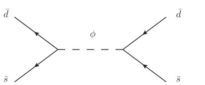
Figure 5: Feynman diagram for the dijet production.

The cross section of the resonance $\phi$ production and decaying into dijet is highly sensitive to the width of $\phi$ decay, which is given by

$$\Gamma_{\phi}=\Gamma_{\phi\to\bar{d}\bar{s}}+\Gamma_{\phi\to u_{i}\bar{\chi}},$$ (25)

with

$$\Gamma_{\phi\to\bar{d}\bar{s}} = \frac{(\lambda_{S}^{12})^{2}}{2\pi}m_{\phi},$$

$$\Gamma_{\phi\to u_{i}\bar{\chi}} = \frac{|a_{S}^{i}|^{2}}{16\pi m_{\phi}^{3}}(m_{\phi}^{2}-m_{u_{i}}^{2}-m_{\chi}^{2})\lambda^{1/2}(m_{\phi}^{2},m_{u_{i}}^{2},m_{\chi}^{2}),$$ (26)

where $\lambda(a,b,c)=a^{2}+b^{2}+c^{2}-2ab-2bc-2ca$. We will take into account the effect of these widths in our numerical calculation below. To calculate the cross section, we use MadGraph5v1.3.3 Alwall et al. (2011) with the effective Lagrangian implemented in by FeynRules Christensen and Duhr (2009). We vary the mass of $\phi$ from 500 GeV to 2500 GeV with a step of 100 GeV. For each mass, we calculate the decay width of $\phi$, assuming $\lambda_{S}^{12}=a_{S}^{3}=0.2,a_{S}^{1}=a_{S}^{2}=0,m_{\chi}=50{~{}\rm GeV}$. Then we change the corresponding parameters in MadGraph and calculate the cross sections of the dijet production. We choose the kinematical cuts as following Khachatryan et al. (2010); Chatrchyan et al. (2011):

$$|\eta_{j}|<2.5,\quad|\eta_{j_{1}}-\eta_{j_{2}}|<1.3.$$ (27)

The cross sections of the dijet signal before and after the cuts are listed in Table. 1.

$m_{\phi}$ (GeV)	500	600	700	800	900	1000	1100
$\sigma_{0}$ (pb)	28.2	12.6	6.11	3.17	1.73	9.80$\times 10^{-2}$	5.71$\times 10^{-2}$
$\sigma_{f}$ (pb)	16.2	7.13	3.52	1.84	9.98$\times 10^{-2}$	5.66$\times 10^{-2}$	3.22$\times 10^{-2}$
$m_{\phi}$ (GeV)	1200	1300	1400	1500	1600	1700	1800
$\sigma_{0}$ (pb)	3.40$\times 10^{-2}$	2.07$\times 10^{-2}$	1.28$\times 10^{-2}$	7.95$\times 10^{-2}$	5.00$\times 10^{-2}$	3.17$\times 10^{-2}$	2.03$\times 10^{-2}$
$\sigma_{f}$ (pb)	1.94$\times 10^{-2}$	1.18$\times 10^{-2}$	7.27$\times 10^{-2}$	4.55$\times 10^{-2}$	2.82$\times 10^{-2}$	1.79$\times 10^{-2}$	1.16$\times 10^{-2}$
$m_{\phi}$ (GeV)	1900	2000	2100	2200	2300	2400	2500
$\sigma_{0}$ (pb)	1.30$\times 10^{-2}$	8.35$\times 10^{-3}$	5.38$\times 10^{-3}$	3.47$\times 10^{-3}$	2.23$\times 10^{-3}$	1.44$\times 10^{-3}$	9.27$\times 10^{-4}$
$\sigma_{f}$ (pb)	7.42$\times 10^{-3}$	4.79$\times 10^{-3}$	3.07$\times 10^{-3}$	1.99$\times 10^{-3}$	1.28$\times 10^{-3}$	8.35$\times 10^{-4}$	5.25$\times 10^{-4}$

Table 1: The cross sections of dijet production induced by the resonance of $\phi$ before ($\sigma_{0}$) and after ($\sigma_{f}$) the cuts given in Eq. (27), assuming $\lambda_{S}^{12}=a_{S}^{3}=0.2,a_{S}^{1}=a_{S}^{2}=0$.

Fig. 6 shows the allowed region of $\lambda_{S}(=\lambda_{S}^{12}=a_{S}^{3})$ as a function of $m_{\phi}$, where we choose the acceptance $\mathcal{A}=0.6$ as in Ref. Chatrchyan et al. (2011). It is required that $\sigma_{jj}\cdot\mathcal{A}$ is not larger than the observed $95\%$ C.L. upper limit in the dijet experiment Khachatryan et al. (2010); Chatrchyan et al. (2011). The bump of the curve in the region from 500 GeV to 1000 GeV for $m_{\phi}$ is due to the fact that we compare with data in this region and the other regions corresponding to integrated luminosities of 2.9 ${\rm pb^{-1}}$ and 1 ${\rm fb^{-1}}$, respectively, collected by the CMS experiment at the LHC.

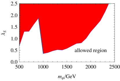
Figure 6: The allowed region of $\lambda_{S}(=\lambda_{S}^{12}=a_{S}^{3})$ by dijet experiments at the LHC as a function of $m_{\phi}$.

III Signal and Background

The signals of the monotop production are

$$pp\to t+{E\!\!\!/}_{T}\to bW+{E\!\!\!/}_{T}\to bjj+{E\!\!\!/}_{T}\quad{\rm and}\quad bl+{E\!\!\!/}_{T},$$ (28)

which are shown in Fig. 7.

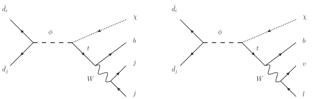
Figure 7: Feynman diagrams for the monotop production.

The symbol $b$ and $j$ denote a $b$-tagged jet and light quark or gluon jet, respectively, and $l$ refers to the first two generation charged leptons, i.e., $e$ and $\mu$. We define the process with top hadronic decay as hadronic mode, while the one with top semileptonic decay as semileptonic mode. The hadronic mode suffers from fewer backgrounds in the SM than the semileptonic mode because of the smaller phase space due to more particles in the final states. This mode has been studied in Ref. Andrea et al. (2011) where they assume the branching fraction $R(\phi\to t\bar{\chi})$ equal to one. However, this assumption is over optimistic. From Eq. (II.3) we get the branching fraction $R(\phi\to t\bar{\chi})$,

$$R(\phi\to t\bar{\chi}) = \frac{\Gamma_{\phi\to t\bar{\chi}}}{\Gamma_{\phi\to t\bar{\chi}}+\Gamma_{\phi\to\bar{d}\bar{s}}}=\frac{1}{1+z},$$ (29)

with

$$z = \frac{8(\lambda_{S}^{12})^{2}}{|a_{S}^{3}|^{2}}\frac{m_{\phi}^{4}}{(m_{\phi}^{2}-m_{t}^{2}-m_{\chi}^{2})\lambda^{1/2}(m_{\phi}^{2},m_{t}^{2},m_{\chi}^{2})}.$$ (30)

Here we assume that the decay widths $\Gamma_{\phi\to u\bar{\chi}}=\Gamma_{\phi\to c\bar{\chi}}=0$. In the case of $\lambda_{S}^{12}=a_{S}^{3}=0.2,m_{t}=173.1{~{}\rm GeV},m_{\phi}=500{~{}\rm GeV}{\rm~{}and~{}}m_{\chi}=50{~{}\rm GeV}$, we find $\Gamma_{\phi\to t\bar{\chi}}=0.300{~{}\rm GeV}$, $\Gamma_{\phi\to\bar{d}\bar{s}}=3.183{~{}\rm GeV}$, and the branching fraction of $\phi\to t\bar{\chi}$ is just about 0.1. So, in this work, we take into account the effect of both $\phi$ decay channels and below we will discuss further the hadronic and leptonic modes in detail.

Before discussing the signal and backgrounds in detail, we first give some comments on the parameter $m_{\chi}$. In the SUSY model, without the assumption of gaugino mass unification, there is no general mass limit from $e^{+}e^{-}$ colliders for the lightest neutralino Nakamura et al. (2010). The indirect constraints from $(g-2)_{\mu}$, $b\to s\gamma$ and $B\to\mu^{+}\mu^{-}$ show that the lightest neutralino mass can be as low as about 6 GeV Belanger et al. (2004). In our case, we choose the default value of $m_{\chi}=50$ GeV and discuss the effect on the discovery significance when varying $m_{\chi}$ in the range $5-100$ GeV. An estimate of the width can be made by the Feynman diagrams shown in Fig. 7, where we can consider only $\chi$ as the initial-state particle, for example,

$$\chi(p_{1})\to d(p_{2})s(p_{3})b(p_{4})\nu(p_{5})l^{+}(p_{6}).$$ (31)

Then the width of $\chi$ is given by

$$\Gamma_{\chi}=\frac{1}{2m_{\chi}}\int|\overline{\mathcal{M}}|^{2}d\Gamma_{5},$$ (32)

where $|\overline{\mathcal{M}}|^{2}$ is the matrix element squared for the decay process which has taken into account the average and sum over the initial- and final-state spins and colors. When the masses of all the final-state particles are neglected, the five body phase space integration can be written as

$$\int d\Gamma_{5} = \frac{1}{32768\pi^{7}}\frac{1}{m_{\chi}^{2}}\int_{0}^{m_{\chi}^{2}}ds_{23}\int_{0}^{(m_{\chi}-\sqrt{s_{23}})^{2}}ds_{456}\int_{0}^{s_{456}}ds_{45}$$ (33)

$$\lambda^{1/2}(m_{\chi}^{2},s_{23},s_{456})\left(1-\frac{s_{45}}{s_{456}}\right),$$

where $s_{ij}=(p_{i}+p_{j})^{2}$ and $s_{ijk}=(p_{i}+p_{j}+p_{k})^{2}$. In the mass range of $\chi$ we are interested in, the momenta of the decay products of the $W$ boson are so small compared with the mass of the $W$ boson that we neglect them in the calculation of the matrix element. Moreover, we assume that the lepton $l^{+}$ carries about one-fifth of the energy of $\chi$ on average. In this case, the matrix element squared is simply given by

$$|\overline{\mathcal{M}}|^{2}\approx\frac{96}{5}g_{W}^{4}(\lambda_{S}^{12})^{2}(a_{S}^{3})^{2}\frac{m_{\chi}^{2}}{m_{\phi}^{4}m_{t}^{2}M_{W}^{4}}s_{23}s_{45}.$$ (34)

where $g_{W}$ is the coupling of the $W$ boson with left-handed fermions. Then we perform the integration in Eq. (32), and obtain

$$\Gamma_{\chi}\approx 1.82\times 10^{-19}{\rm GeV}\left(\frac{\lambda_{S}^{12}}{0.2}\right)^{2}\left(\frac{a_{S}^{3}}{0.2}\right)^{2}\frac{(m_{\chi}/50{\rm GeV})^{11}}{(m_{\phi}/500{\rm GeV})^{4}(m_{t}/173.1{\rm GeV})^{2}(M_{W}/80.4{\rm GeV})^{4}}.$$ (35)

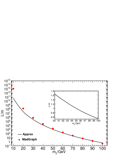
Figure 8: The distance travelled by the particle $\chi$ before its decay as a function of its mass. The solid line is obtained from Eq. (35) while the dots denote the results of MadGraph. The relevant parameters are chosen as $\lambda_{S}^{12}=a_{S}^{3}=0.2$, $m_{t}=173.1{~{}\rm GeV},M_{W}=80.4{~{}\rm GeV},{\rm~{}and~{}}m_{\phi}=500{~{}\rm GeV}$.

The produced $\chi$ at hadron colliders, as a decay product of a massive particle, usually has such a large energy that it moves nearly in the speed of light. In Fig. 8, we show the distance travelled by the particle $\chi$ before its decay as a function of its mass. It can be seen that the distance strongly depends on the mass of $\chi$ and decreases with increasing $m_{\chi}$. The results of MadGraph are well approximated by those obtained from Eq. (35) except for the low mass region since we have neglected the mass of final-state particle in Eq. (35). But this discrepancy between them in the low mass region is not important because they are both much larger than the size of the detector at the LHC. The ATLAS collaboration has searched for displaced vertices arising from decays of new heavy particles and found that the efficiency for detecting displaced vertices almost vanishes for a distance between the primary and the displaced vertex larger than 0.35 m Aad et al. (2012). Therefore, as shown in Fig. 8, it is reasonable that the particle $\chi$ with a mass less than 100 GeV is considered as missing energy at the LHC.

III.1 Hadronic mode

For the hadronic mode, the main backgrounds arise from $pp\to jjjZ(\nu\bar{\nu})$, with a jet misidentified as a $b$-jet, and $pp\to b\bar{b}jZ(\nu\bar{\nu})$ with a $b$-jet not tagged. The top pair and single top production processes with hadronic top quark decay may also contribute to the backgrounds if some jets are not detected. The signal and backgrounds are simulated by MadGraph5v1.3.3 Alwall et al. (2011) and ALPGEN Mangano et al. (2003) interfaced with PYTHIA Sjostrand et al. (2008, 2006) to perform the parton shower and hadronization. In this mode, the momentum of three jets, and therefore momentum of the $W$ boson and top quark, can be reconstructed, which leads to efficient event selection using invariant mass cut. In the following numerical calculation, the default relevant parameters are chosen as $\lambda_{S}^{12}=a_{S}^{3}=0.2,\lambda_{S}^{13}=\lambda_{S}^{23}=0,a_{S}^{1}=a_{S}^{2}=0,m_{t}=173.1{~{}\rm GeV},m_{\phi}=500{~{}\rm GeV}{\rm~{}and~{}}m_{\chi}=50{~{}\rm GeV}$, and CTEQ6L1 PDF is used. The renormalization and factorization scales are set at $m_{\phi}$. We use the following basic selection cuts

$$p_{T}^{b,j}>30{~{}\rm GeV},\quad|\eta^{b,j}|<2.4,\quad{\Delta R}_{bb,bj,jj}>0.5.$$ (36)

Moreover, we choose a $b$-tagging efficiency of 50$\%$ while the misidentification rates for other jets are, 8$\%$ for charm quark, 0.2$\%$ for gluon and other light quarks Aad et al. (2009).

To determine the missing transverse energy cut, we show the normalized spectrum of the missing transverse energy for the signal and backgrounds in Fig. 9. The backgrounds concentrate in the region ${E\!\!\!/}_{T}<100{~{}\rm GeV}$ because the missing transverse energy of the background comes from either an invisible decayed $Z$ boson or non-detected jets, which are produced mainly via t-channel. In contrast, the missing transverse energy of the signal results from the decay of a heavy resonance so that it can be large. Therefore we choose the missing transverse energy cut

$${E\!\!\!/}_{T}>100{~{}\rm GeV}.$$ (37)

Meanwhile, the shape of the signal is similar to the distribution ${E\!\!\!/}_{T}/\sqrt{{{E\!\!\!/}_{T}^{max}}^{2}-{E\!\!\!/}_{T}^{2}}$ with an edge at ${E\!\!\!/}_{T}^{max}=\lambda^{1/2}(m_{\phi}^{2},m_{t}^{2},m_{\chi}^{2})/2m_{\phi}$. This feature may help to specify the masses of the resonance and the missing particle.

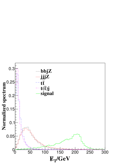
Figure 9: The normalized spectrum of missing transverse energy in the hadronic mode at the LHC ($\sqrt{s}=$ 7 TeV).

In Fig. 10 we show the reconstructed top quark mass distribution for the signal and backgrounds processes using the three leading jets.

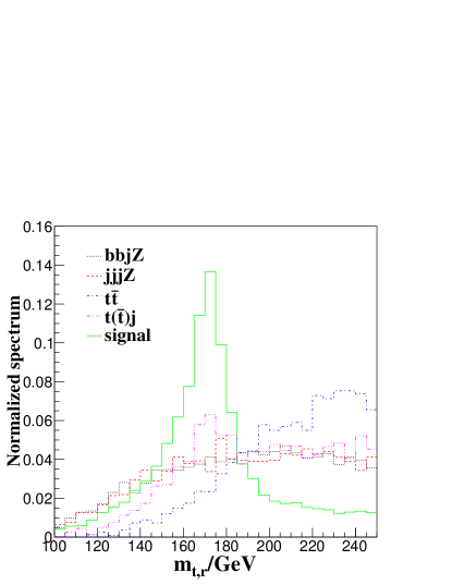
Figure 10: The reconstructed top quark mass distribution for the signal and backgrounds processes.

It can be seen that there is a peak around $175$ GeV for the signal while the distributions of backgrounds grow up with the increase of reconstructed top quark mass, and thus we impose the invariant mass cut in the final states as following,

$$120~{}{\rm GeV}<m_{t,r}<200~{}{\rm GeV}.$$ (38)

The cross sections of the signal and backgrounds after various cuts at the LHC ($\sqrt{s}=$ 7 TeV) are listed in Table 2. It can be seen that the backgrounds decrease dramatically when the invariant mass cuts are imposed, and the cross section of $b\bar{b}jZ(\nu\bar{\nu})$ is not smaller than that of $jjjZ(\nu\bar{\nu})$ after all cuts imposed so that it can not be neglected. The $t\bar{t}$ and $t(\bar{t})j$ processes are mainly suppressed by the missing transverse energy cut, which can be seen from Fig. 9.

To investigate the discovery potential of monotops in the hadronic mode at the LHC ($\sqrt{s}=$ 7 TeV) with an integrated luminosity of 1 $\rm fb^{-1}$, in Fig. 11 we present the contour curves of significance $\mathcal{S}=S/\sqrt{B}$ versus the parameters $\lambda_{S}^{12}$ and $a_{S}^{3}$, where $S$ and $B$ are respectively the expected numbers of the signal and backgrounds events. And in Fig. 12 we present the $5\sigma$ ($\mathcal{S}=5$) discovery limits of $m_{\phi}$, $m_{\chi}$ and $\lambda_{S}^{12}=a_{S}^{3}=\lambda_{S}$. From Fig. 11 we can see that for a $5\sigma$ discovery, the sensitivity to $\lambda_{S}^{12}$ and $a_{S}^{3}$ can be as low as 0.02 and 0.06, respectively. And from Fig. 12, we find that the LHC can generally detect the coupling $\lambda_{S}$ down to lower than 1.0 for $m_{\phi}$ less than 1.4 TeV. For $m_{\phi}$ larger than 1.4 TeV, the coupling $\lambda_{S}$ needed to discovery the monotop signal increases quickly. The increase of the integrated luminosity has a larger impact for larger $m_{\phi}$. Moreover, the narrow bands of the lines, which correspond to the value of $m_{\chi}$ varying from 5 GeV to 100 GeV, indicate the weak dependence of the discovery potential on the value of $m_{\chi}$ if $m_{\chi}\ll m_{\phi}$.

In this mode, since the full kinematic information of the top quark can be reconstructed, the mass of the resonance $\phi$ can be obtained by

$$m_{\phi}=\sqrt{p_{t}^{2}+m_{\chi}^{2}}+\sqrt{p_{t}^{2}+m_{t}^{2}},$$ (39)

with

$$p_{t}^{2}=p_{t,x}^{2}+p_{t,y}^{2}+p_{t,z}^{2},$$ (40)

in which $p_{t,x},p_{t,y},p_{t,z}$ are the three-vector momentum of the top quark. Fig. 13 shows the distribution of the reconstructed $m_{\phi}$. We can see a peak around $m_{\phi}=500$ GeV in the signal. To illustrate the effect of $m_{\chi}$, we also plot the situation that $m_{\chi}=0$ GeV is assumed in Eq. (39) when reconstructing $m_{\phi}$. It is evident that the peak position does not changed. This information, combined with the missing transverse energy distribution, may help to specify the masses of the resonance and the missing particle.

$\sigma$ (fb)	basic	${E\!\!\!/}_{T}$	$m_{t,r}$	b-tagging	$\epsilon_{cut}$
signal	902	811	502	251	27.1$\%$
$jjjZ(\nu\bar{\nu})$	$7.03\times 10^{4}$	$7.87\times 10^{3}$	944	9.35	0.013$\%$
$b\bar{b}jZ(\nu\bar{\nu})$	$1.70\times 10^{3}$	143	19.4	9.67	0.57$\%$
$t\bar{t}$	$2.80\times 10^{4}$	$34.6$	0.28	0.14	5 $\times 10^{-6}$
$t(\bar{t})j$	$2.35\times 10^{4}$	$10.9$	0.24	0.12	5 $\times 10^{-6}$

Table 2: The cross sections of the signal and backgrounds after various cuts in the hadronic mode at the LHC ($\sqrt{s}=$ 7 TeV). The cut acceptance $\epsilon_{cut}$ is also listed. The entries after the $m_{t,r}$ cut for $t\bar{t}$ and $t(\bar{t})j$ processes are estimated by considering that one out of the total events we have generated for analysis can survive various kinematic cuts.

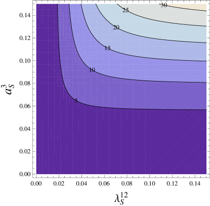
Figure 11: The significance in the hadronic mode at the LHC ($\sqrt{s}=$ 7 TeV) with an integrated luminosity of 1 $\rm fb^{-1}$ versus the parameters $\lambda_{S}^{12}$ and $a_{S}^{3}$, assuming $m_{\phi}=500{~{}\rm GeV}{\rm~{}and~{}}m_{\chi}=50{~{}\rm GeV}$.

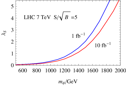
Figure 12: The $5\sigma$ discovery limits of $m_{\phi}$ and $\lambda_{S}(=\lambda_{S}^{12}=a_{S}^{3})$ in the hadronic mode at the LHC ($\sqrt{s}=$ 7 TeV). Either band consists of twenty solid lines from the bottom up corresponding to the value of $m_{\chi}$ varying from 5 GeV to 100 GeV with a step of 5 GeV.

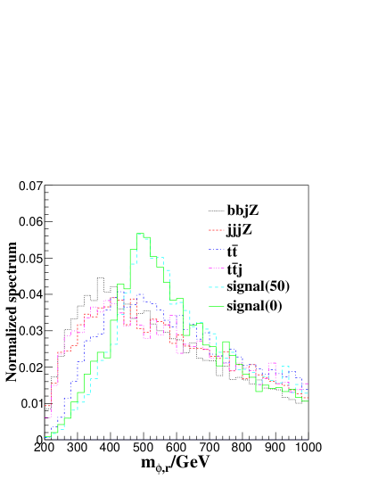
Figure 13: The reconstructed $m_{\phi}$ distribution for the signal and backgrounds processes. The signal(50) and signal(0) represent that the values of $m_{\chi}$ in Eq. (39) are 50 GeV and 0 GeV, respectively.

III.2 Semileptonic mode

For the semileptonic mode, the dominant backgrounds are $pp\to W(l\nu)j$ with the jet misidentified as a $b$-jet and single top production with semileptonic top quark decay. The $Wj$ background is very large because there are only two final-state particles, compared with four final-state particles in $pp\to jjjZ$ and $pp\to b\bar{b}jZ$ processes. Besides, the final state of the signal contains two missing particles, which makes the reconstruction of the mass of the top quark very challenging. Nevertheless, the semileptonic mode is still promising once appropriate cuts are imposed. The signal and backgrounds are simulated by MadGraph5v1.3.3 Alwall et al. (2011) interfaced with PYTHIA Sjostrand et al. (2008). We choose the same default parameters as in hadronic mode, and the basic cuts are

$$p_{T}^{b}>30{~{}\rm GeV},\quad|\eta^{b,l}|<2.4,\quad{\Delta R}_{bl}>0.5.$$ (41)

Fig. 14 shows the normalized spectrum of the transverse momentum of the charged lepton in the semileptonic mode at the LHC with $\sqrt{s}=$ 7 TeV. We can see that it is difficult to suppress the backgrounds by $p_{T}^{l}$ cut because of the similar distributions of the signal and backgrounds. As a result, we choose a loose cut

$$p_{T}^{l}>20{~{}\rm GeV}$$ (42)

to keep more signal events.

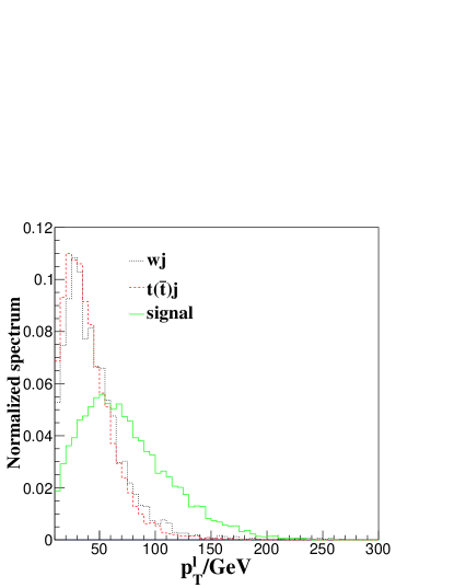
Figure 14: The normalized spectrum of transverse momentum of the charged lepton in the semileptonic mode at the LHC ($\sqrt{s}=$ 7 TeV).

Fig. 15 shows the normalized spectrum of the missing transverse energy in the semileptonic mode at the LHC with $\sqrt{s}=$ 7 TeV. The backgrounds decrease while the signal increases in the range $30{~{}\rm GeV}<{E\!\!\!/}_{T}<150{~{}\rm GeV}$. The reason is that the missing particle of the backgrounds is (anti)neutrino, which comes from the $W$ boson, and the $Wj$ is mainly produced through t-channel, in which the momentum of final-state particles tend to be collinear to those of the initial-state particles. The situation for the single top production is similar. In contrast, the missing particles of the signal originate from a resonance of a large mass, and thus could be produced with large transverse momentum. Therefore, we impose the missing transverse energy cut

$${E\!\!\!/}_{T}>120{~{}\rm GeV}$$ (43)

to suppress the backgrounds.

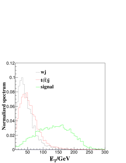
Figure 15: The normalized spectrum of the missing transverse energy in the semileptonic mode at the LHC ($\sqrt{s}=$ 7 TeV).

Fig. 16 shows the normalized spectrum of the transverse mass, which is defined as Nakamura et al. (2010)

$$M_{T}=\sqrt{({E\!\!\!/}_{T}+E_{T}^{l})^{2}-(\vec{{p\!\!\!/}}_{T}+\vec{p_{T}^{l}})^{2}},$$ (44)

in the semileptonic mode at the LHC with $\sqrt{s}=$ 7 TeV. The backgrounds increase in the range $0<M_{T}<80{~{}\rm GeV}$ and have a peak around $M_{T}\sim 80{~{}\rm GeV}$. This is due to the fact that the transverse mass measure the maximum of the invariant mass of the missing particles and the lepton, which is the mass of $W$ boson for the backgrounds. In contrast, the signal concentrates in the range $M_{T}>100{~{}\rm GeV}$. Thus, to suppress the backgrounds efficiently, we impose the transverse mass cut

$$M_{T}>120{~{}\rm GeV}.$$ (45)

Figure 16: The normalized spectrum of the transverse mass $M_{T}$ in the semileptonic mode at the LHC ($\sqrt{s}=$ 7 TeV).

The cross sections of the signal and backgrounds after various cuts at the LHC ($\sqrt{s}=$ 7 TeV) are listed in Table 3. We can see that the backgrounds nearly vanish after the transverse mass cut is imposed, which means that it is very promising to search for the signal of monotops in the semileptonic mode. In Fig. 17, we show the contour curves of the significance $\mathcal{S}$ versus the parameters $\lambda_{S}^{12}$ and $a_{S}^{3}$ in the semileptonic mode at the LHC ($\sqrt{s}=$ 7 TeV). And in Fig. 18, we show the $5\sigma$ ($\mathcal{S}=5$) discovery limits of $m_{\phi}$, $m_{\chi}$ and $\lambda_{S}^{12}=a_{S}^{3}=\lambda_{S}$ in the semileptonic mode. From Fig. 17 we can see that for a $5\sigma$ discovery, the sensitivity to $\lambda_{S}^{12}$ and $a_{S}^{3}$ can be as low as 0.015 and 0.045, respectively, which are smaller than the corresponding values in the hadronic mode. And from Fig. 18, we find that the LHC can generally detect the coupling $\lambda_{S}$ down to lower than 0.4 for $m_{\phi}$ less than 1.4 TeV, and for larger $m_{\phi}$, the coupling $\lambda_{S}$ needed to discover the monotop signal increases quickly. Also, the value of $m_{\chi}$ has little effect on the discovery potential.

$\sigma$ (fb)	basic	$p_{T}^{l}$	${E\!\!\!/}_{T}$	$M_{T}$	b-tagging	$\epsilon_{cut}$
signal	399	376	231	218	109	27.3$\%$
$W(l\nu)j$	$1.83\times 10^{6}$	$1.53\times 10^{6}$	$3.45\times 10^{4}$	$1.83$	0.003	2$\times 10^{-9}$
$t(\bar{t})j$	$9.09\times 10^{3}$	$7.33\times 10^{3}$	$185$	$2.15$	1.08	$0.012\%$

Table 3: The cross sections of the signal and backgrounds after various cuts in the semileptonic mode at the LHC ($\sqrt{s}=$ 7 TeV). The cut acceptance $\epsilon_{cut}$ is also listed. The entries after the $M_{T}$ cut for $W(l\nu)j$ process are estimated by considering that one out of the total events we have generated for analysis can survive various kinematic cuts.

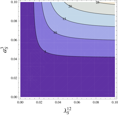
Figure 17: The significance in the semileptonic mode at the LHC ($\sqrt{s}=$ 7 TeV) with an integrated luminosity of 1 $\rm fb^{-1}$ versus the parameters $\lambda_{S}^{12}$ and $a_{S}^{3}$, assuming $m_{\phi}=500{~{}\rm GeV}{\rm~{}and~{}}m_{\chi}=50{~{}\rm GeV}$.

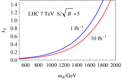
Figure 18: The $5\sigma$ discovery limits of $m_{\phi}$ and $\lambda_{S}(=\lambda_{S}^{12}=a_{S}^{3})$ in the semileptonic mode at the LHC ($\sqrt{s}=$ 7 TeV). Either band consists of twenty solid lines from the bottom up corresponding to the value of $m_{\chi}$ varying from 5 GeV to 100 GeV with a step of 5 GeV.

IV Conclusion

We have investigated the potential of the early LHC to discover the signal of monotop production. First, we obtain the parameter space of the effective Lagrangian constrained by the present data of $Z$ boson hadronic decay branching ratio, $K^{0}-\overline{K^{0}}$ mixing and dijet productions at the LHC. Then, we study the various cuts imposed on the events, reconstructed from the hadronic final states, to suppress backgrounds and increase the significance in detail. And we find that in the hadronic mode the information from the missing transverse energy and reconstructed resonance mass distributions can be used to specify the masses of the resonance and the missing particle. Lastly, we present the significance $\mathcal{S}$ at the LHC ($\sqrt{s}=$ 7 TeV) with an integrated luminosity of 1 $\rm fb^{-1}$ in the parameter space allowed by the current data, and the $5\sigma$ discovery limits of $m_{\phi}$ and $\lambda_{S}(=\lambda_{S}^{12}=a_{S}^{3})$. Our results show that the LHC can generally detect the coupling $\lambda_{S}$ down to lower than 1.0 and 0.4 for $m_{\phi}$ less than 1.4 TeV in the hadronic and semileptonic modes, respectively.