The size of the jet launching region in M87

Abstract

The supermassive black hole candidate at the center of M87 drives an ultra-relativistic jet visible on kiloparsec scales, and its large mass and relative proximity allow for event horizon scale imaging with very long baseline interferometry at millimetre wavelengths (mm-VLBI). Recently, relativistic magneto-hydrodynamic (MHD) simulations of black hole accretion flows have proven capable of launching magnetically-dominated jets. We construct time-dependent disc/jet models of the innermost portion of the M87 nucleus by performing relativistic radiative transfer calculations from one such simulation. We identify two types of models, jet-dominated or disc/jet, that can explain the spectral properties of M87, and use them to make predictions for current and future mm-VLBI observations. The Gaussian source size for the favored sky orientation and inclination from observations of the large-scale jet is $33-44\mu$as ($\simeq 4-6$ Schwarzschild radii) on current mm-VLBI telescopes, very similar to existing observations of Sgr A*. The black hole shadow, direct evidence for an event horizon, should be visible in future measurements using baselines between Hawaii and Mexico. Both models exhibit variability at millimetre wavelengths with factor of $\simeq 2$ amplitudes on year timescales. For the low inclination of M87, the counter-jet dominates the event horizon scale millimetre wavelength emission from the jet-forming region.

1 Introduction

Messier 87 (M87) is a giant elliptical galaxy in the Virgo cluster, known for its galaxy-scale, ultra-relativistic jet. Very long baseline interferometry (VLBI) images at 7mm (Junor, Biretta & Livio, 1999; Ly, Walker & Wrobel, 2004; Walker et al., 2008) show extended jet structure on milli-arcsecond (mas) scales, emanating from an unresolved bright core. Recent images between $7$ mm and $1.3$ cm (Hada et al., 2011) suggest that this core is coincidental with the central black hole candidate (hereafter M87 refers to the black hole rather than the galaxy). M87 is also one of the two largest black holes on the sky (along with the Galactic centre black hole candidate, Sgr A*). Its mass is $\simeq 6.4\times 10^{9}M_{\odot}$ (Gebhardt & Thomas, 2009; Gebhardt et al., 2011), $\sim$1600 times larger than Sgr A*. At a distance of $16$ Mpc, the angular size, $\delta\theta\propto M/D$, is about 4/5 that of Sgr A*.

Recent VLBI observations at $1.3$ mm have detected source structure in Sgr A* on event horizon scales (Doeleman et al., 2008; Fish et al., 2011), allowing a direct comparison between observations and black hole accretion theory (e.g., Dexter et al., 2010; Broderick et al., 2011). These observations also have the potential to detect the black hole shadow (Bardeen, 1973; Falcke, Melia & Agol, 2000; Dexter et al., 2010), which would provide the first direct evidence for an event horizon.

M87 is just as, if not more, promising a mm-VLBI target as Sgr A*. M87 is in the Northern sky, offering longer mutual visibility with current telescopes. Its large black hole mass gives a proportionally longer dynamical time, so that its event horizon spans $\sim$1 light-day. This means that, unlike in Sgr A*, Earth-aperture synthesis could be used to fill in the u-v plane, potentially (with additional telescopes) allowing the creation of an image of the source directly, in contrast with the model-dependent Fourier domain fitting techniques necessary for Sgr A*. Micro-arcsecond ($\mu$as) resolution of mm-VLBI also offers the possibility of imaging the jet launching region, which would provide the opportunity to compare directly with physical models of jet formation in the immediate vicinity of the black hole. The most recent mm-VLBI campaign observed M87 as well as Sgr A* (Fish et al., 2011), but the data are as yet unpublished.

The spectral properties of M87 are well known: it is an inverted radio source with a power law tail extending from the spectral peak in the millimetre to the optical. Previous semi-analytic work has modeled the low-frequency radio emission as arising from synchrotron radiation in either an advection-dominated accretion flow (Reynolds et al., 1996; Di Matteo et al., 2003) or a “truncated” accretion disc (Yuan, 2000; Broderick & Loeb, 2009). Both types of models can fit the spectrum. Synthetic jet images have also been produced as predictions for mm-VLBI from one of these semi-analytic models (Broderick & Loeb, 2009).

Maps of synchrotron emission from numerical simulations of jets have also been compared to observations of M87 (Zakamska, Begelman & Blandford, 2008; Gracia et al., 2009), but these jets are input by hand rather being formed self-consistently from an accretion flow. Conversely, axisymmetric general relativistic MHD (GRMHD) simulations of the accretion flow have been used to fit the spectrum of the core (Mościbrodzka et al., 2011; Hilburn & Liang, 2011).

Jet formation has recently become accessible to global, 3D GRMHD simulations (McKinney & Blandford, 2009). In their simulation initialised with a dipolar magnetic field (MBD in Dexter et al., 2010, and here), an ultra-relativistic jet is produced self-consistently from an accretion disc and propagates stably out to $1000$ M before it interacts with the simulation boundary. We perform general relativistic radiative transfer via ray tracing to create the first time-dependent spectral models of M87 from a GRMHD simulation, and use the models to make predictions for current and future mm-VLBI observations. The simulation and the relativistic radiative transfer method used to compute observables are described in §2, along with the details of the radiative disc/jet models. Fiducial models for the M87 spectrum are identified in §3, and the resulting millimetre images and variability are studied in §4 and §5. The implications of our results are discussed in §6 along with the many uncertainties in constructing the models. We summarize the results in §7.

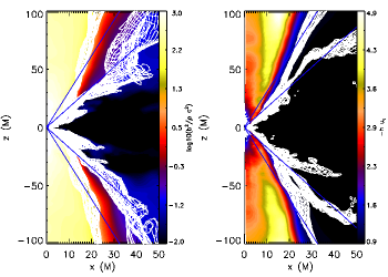
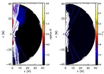
Figure 1: Ratio of magnetic to rest energy density (first and third panels) and specific enthalpy measured at infinity (second and fourth panels) for single time steps of the MBD (left two panels) and MBQ (right two panels) simulations. The azimuthally averaged data are shown in colour, while contours of $b^{2}/\rho c^{2}=0.1$, $8\pi$ and $-hu_{t}=1.0,1.1$ for the full range of azimuths are overplotted. Also overplotted in blue are lines of constant polar angle, $\theta=18^{\circ}$, $30^{\circ}$. For M87, $1$ M $\simeq 4\mu$as. The jet is clearly identified in MBD, but only roughly corresponds to lines of constant $\theta$. There is no persistent jet in the MBQ simulation.

2 Methods

2.1 Simulation Data

McKinney & Blandford (2009) carried out 3D global GRMHD simulations starting from a hydrostatic torus in whose angular momentum was aligned with the black hole spin axis for a spin value $a/M=0.92$. The initial torus pressure maximum was located at $r=12$ M. The GRMHD code used was a 3D version of HARM (Gammie, McKinney & Tóth, 2003; Noble et al., 2006) with fourth order interpolation and time-stepping (McKinney, 2006b) as well as other improvements (McKinney, 2006a; Tchekhovskoy, McKinney & Narayan, 2007).

This simulation conserved total energy and neglected radiative cooling. Energy-conserving simulations convert the energy lost to grid-scale numerical magnetic reconnection into heat. This is appropriate for studying radiatively inefficient sources such as Sgr A* or M87, where the accretion flow is hot and geometrically thick. The full azimuthal domain was included, but only marginally resolved with a resolution of 256$\times$128$\times$32 in ($r$, $\theta$, $\phi$). The effective resolution was higher than in fully second order schemes due to the high order scheme used. The coordinates were regular but warped, with the resolution concentrated toward the mid-plane at small radius to resolve the disc and towards the pole at large radius to resolve the jet. The total duration was $3500$ M, with roughly constant radial profiles in accretion rate and angular momentum out to $r\simeq 10$ M by $t\sim 3000$ M. The snapshot used for spectral fitting in §3 is from $t=3000$ M, after an approximate quasi-steady state was established in the inner disc. The final $2000$ M of the simulation is considered when we study time-variable properties of the radiative models.

2.2 Ray Tracing

We performed relativistic radiative transfer on the simulation data via ray tracing using the code grtrans (Dexter, 2011). Starting from an observer’s camera, rays are traced backwards in time toward the black hole assuming they are null geodesics (geometric optics approximation), using the public code geokerr described in Dexter & Agol (2009). In the region where rays intersect the accretion flow, the radiative transfer equation is solved along the geodesic (Broderick, 2006) in the form given in Fuerst & Wu (2004), which then represents a pixel of the image. This procedure is repeated for many rays to produce an image, and at many time steps of the simulation to produce time-dependent images (movies). Light curves are computed by integrating over the individual images. Repeating the procedure over observed wavelengths gives a time-dependent spectrum.

To calculate fluid properties at each point on a ray, the spacetime coordinates of the geodesic are transformed from Boyer-Lindquist to the modified Kerr-Schild coordinates used in the simulation (McKinney, 2006b). Since the accretion flow is dynamic, light travel time delays along the geodesic are taken into account. Data from the sixteen nearest zone centres (eight on the simulation grid over two time steps) were interpolated to each point on the geodesic.

2.3 Radiative Modeling

Computing emission and absorption coefficients requires converting simulation fluid variables (pressure/internal energy, mass density, and magnetic field strength) into an electron distribution function in physical units. The black hole mass sets the length and time scales, while the mass of the initial torus provides an independent scale and fixes the accretion rate. The scalings are such that $n$ and $b^{2}$ are proportional to the accretion rate. There is no consensus for the electron distribution or geometry responsible for the millimetre emission in M87. The presence of an extended jet at $7$ mm indicates that the jet is at least comparable in luminosity to the disc at that wavelength. Since our model consists of a GRMHD simulation where a jet is produced from accretion onto a black hole, we also include a disc component. The emission mechanism is taken to be entirely synchrotron radiation for both components. The disc electrons are assumed to be thermal, obeying a relativistic Maxwell (Maxwell–Juttner) distribution. As in previous models for Sgr A*, we assume a two-temperature flow with a constant ion-electron temperature ratio which is left as a free parameter (Goldston, Quataert & Igumenshchev, 2005; Mościbrodzka et al., 2009; Dexter et al., 2010). With this parameter, the electron temperature is computed from the gas pressure in the simulation using the ideal gas law. We use the approximate angle-dependent, unpolarized emissivity from Leung, Gammie & Noble (2011). Previous models of M87 have also included non-thermal disc emission, which could be important for explaining the radio spectrum (Broderick & Loeb, 2009).

Figure 2: Sample disc/jet spectra varying each parameter independently: $\gamma_{\text{min}}$ (top left), $p$ (top middle), $\eta$ (top right), $\dot{m}$ (bottom left, in units of $10^{-5}$), and $T_{i}/T_{e}$ (bottom right). The default parameter values are $\gamma_{\text{min}}=50$, $p=3.25$, $\eta=0.05$, $\dot{m}=10\times 10^{-5}$ and $T_{i}/T_{e}=10$.

2.4 Jet Emission

We assume that the jet emission is from non-thermal electrons, whose particle distribution is a power law in electron energy (Lorentz factor) with a constant index $p$ between low- and high-energy cutoffs, $\gamma_{\text{min},\text{max}}$. The unpolarized synchrotron emission and absorption coefficients, $j_{\nu}$ and $\alpha_{\nu}$, for this distribution in cgs units are (Legg & Westfold, 1968; Yuan, Quataert & Narayan, 2003; Dexter, 2011),

$$j_{\nu}=\frac{ne^{2}(p-1)\nu_{c}}{2\sqrt{3}c(\gamma_{\text{min}}^{1-p}-\gamma_{\text{max}}^{1-p})}\left(\frac{\nu}{\nu_{c}}\right)^{-\frac{p-1}{2}}$$

$$\times\left[G(x_{\text{min}})-G(x_{\text{max}})\right],$$ (1)

$$\alpha_{\nu}=\frac{ne^{2}(p-1)(p+2)}{4\sqrt{3}mc\nu_{c}(\gamma_{\text{min}}^{1-p}-\gamma_{\text{max}}^{1-p})}\left(\frac{\nu}{\nu_{c}}\right)^{-\frac{p}{2}-2}$$

$$\times\left[Ga(x_{\text{min}})-Ga(x_{\text{max}})\right],$$ (2)

with $\nu_{c}=\frac{3eB\sin{\theta}}{4\pi mc}$, $x_{\text{min},\text{max}}=\nu/(\gamma_{\text{min},\text{max}}^{2}\nu_{c})$, $\nu$ is the emitted frequency, $n$ is the particle density, $B$ is the magnetic field strength, $\theta$ is the angle between the photon wave-vector and the magnetic field, and the power law synchrotron integrals are,

$$G(x) =\int_{x}^{\infty}dzz^{\frac{p-3}{2}}F(z),$$ (3)

$$Ga(x) =\int_{x}^{\infty}dzz^{\frac{p}{2}-1}F(z),$$ (4)

and where,

$$F(x)=x\int_{x}^{\infty}dyK_{5/3}(y),$$ (5)

is the unpolarized synchrotron function and $K_{\alpha}(y)$ is a modified Bessel function. The functions $G(x)$ and $Ga(x)$ are tabulated for the desired values of $p$ and interpolated for the emissivity calculation. Evaluating the double integrals for constructing the interpolation tables can be sped up significantly using (Westfold, 1959),

$$\int_{x}^{\infty}d\xi\xi^{s-1}\int_{\xi}^{\infty}dy K_{\alpha}(y)=\frac{\alpha+s}{s}\int_{x}^{\infty}d\xi\xi^{s-1}K_{\alpha}(\xi)$$

$$-\frac{x^{s}}{s}\left[\int_{x}^{\infty}dyK_{\alpha+1}(y)-K_{\alpha}(x)\right]$$ (6)

to convert them to sums of single integrals. This form for the absorption coefficient is original, derived in the same fashion as for the emissivity in previous work. Both coefficients reduce to the standard approximate forms when $x_{\text{min}}=0$ and $x_{\text{max}}\rightarrow\infty$.

This form of the emissivity is more accurate for M87 than approximate forms commonly found in the literature that assume a frequency far from those corresponding to the cutoff Lorentz factors. In M87, the frequency corresponding to the low-energy Lorentz factor cutoff, for $\gamma_{\text{min}}=10-100$, is $\nu_{0}\simeq 10^{10-11}$Hz, close to the frequencies of interest for mm-VLBI ($230$ GHz and $345$ GHz). Taking the low-frequency cutoff into account broadens the spectrum and smoothes the turnover from optically thick to thin.

The magnetic field strength everywhere is taken directly from the simulation. For the jet emission, we need to calculate a non-thermal particle density. In magnetically-dominated regions such as the jet, the particle density and internal energy from the simulations are highly inaccurate due to the artificially enforced floor values used for numerical stability. Instead of using these compromised values, we scale the internal energy to the magnetic energy with a constant of proportionality, $\eta$ (cf. Broderick & McKinney, 2010):

$$u_{\text{nth}}=\eta\frac{b^{2}}{8\pi},$$ (7)

where $u_{\text{nth}}$ is the non-thermal internal energy density and $b$ is the magnetic field strength in cgs units. Then the particle density, $n_{\text{nth}}$, is taken from,

$$n_{\text{nth}}=\eta\frac{b^{2}}{8\pi}\frac{p-2}{p-1}(m_{e}c^{2}\gamma_{\text{min}})^{-1},$$ (8)

where $m_{e}$ is the electron mass and which implicitly assumes that all of the internal energy is in electrons, or equivalently that the thermal energy in all particles is negligible and that the positive charge carriers are thermal.

For self-consistency, the rest energy of these non-thermal particles should still be less than the magnetic energy density. This leads to the condition,

$$\eta\lesssim\frac{m_{e}}{m_{e,p}}\frac{p-1}{p-2}8\pi\gamma_{\text{min}},$$ (9)

where $m_{e,p}$ correspond to leptons (baryons) producing the jet. The strictest condition on $\eta$ is found by assuming a baryonic jet, in which case (for $p=3-3.5$),

$$\eta\lesssim.25\frac{\gamma_{\text{min}}}{10}.$$ (10)

This inequality is satisfied in all our models as the maximum $\eta$ considered is $0.1$.

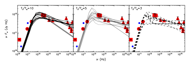
Figure 3: Viable spectra with $T_{i}/T_{e}=10$ (left), $5$, (middle), $3$ (right). The large red symbols are the observational data used as either upper limits (squares), data points (circles) or waveband-averaged data points (triangles). The small blue circles are the flux in the unresolved radio core of VLBI observations.

2.5 Disc/Jet Boundary

The GRMHD simulation consists of a solution for a single component fluid, neglecting electrons and dynamical effects on the local particle distribution. Defining a disc/jet solution then requires choosing a condition for the boundary between the two components. There are a few possibilities.

The general structure of numerical simulations of black hole accretion flows consists of a dense, thick disc with scale height $H/R\sim 0.2-0.3$ centered on the equatorial plane, surrounded by a tenuous wind and then a polar jet. One straightforward method is to define the disc/jet boundary at a particular polar angle ($\simeq 30^{\circ}$).

The outflows in GRMHD simulations arise in magnetically-dominated regions (De Villiers et al., 2005; McKinney, 2006b). The second method is then to define the jet as anywhere that $b^{2}/\rho c^{2}>f$, where $f\simeq 0.1-8\pi$ depending how much of the “disc wind” is to be included in the jet.

Finally, the disc/jet components can be separated as the boundary between inflow/outflow. In this case, unbound fluid elements constitute the jet ($-hu_{t}>1$, where $h$ is the specific enthalpy and $u_{t}$ is the time-component of the covariant fluid four-velocity, De Villiers et al. 2005). Any combination of these criteria can also be used. A comparison of the three criteria for an azimuthally-averaged time step of the simulation is shown in Figure 1, and as expected they all lead to roughly the same definition of the jet for MBD. The inflow/outflow and magnetically-dominated criteria are in particularly good agreement, while the constant slice in polar angle tends to cut out a significant amount of the jet base crucial for mm-VLBI images. We also show the same criteria applied to the simulation from McKinney & Blandford (2009) initialised with a large-scale quadrupolar magnetic field (MBQ in Dexter et al., 2010), where no persistent jet forms. Little of the polar region in this simulation would qualify as a jet by our criteria that fluid be magnetically-dominated or unbound.

In the fiducial models discussed below, we use the condition $b^{2}/\rho c^{2}>1$, but our results are insensitive to the exact criterion used to separate the disc and jet components.

2.6 Model Parameters

These are the required elements to define a radiative model of M87. Unlike in Sgr A*, the inclination of M87 is fairly well constrained from observed superluminal motion in the jet (Heinz & Begelman, 1997), implying $i\lesssim 30^{\circ}$. We fix $i=25^{\circ}$ in this work, but discuss the effect of varying it in § 6.3. The black hole spin is also fixed at $a/M=0.92$ since we only consider models from the MBD simulation.

Each radiative model of M87 then has the following parameters: the ion-electron temperature ratio $T_{i}/T_{e}$ for the disc component, the accretion rate $\dot{M}$ and the disc/jet boundary selection criterion for both components, and $\gamma_{\text{min},\text{max}}$, $p$, and $\eta$ for the jet component. We fix $\gamma_{\text{max}}=10^{5}$ throughout (see Broderick & Loeb, 2009), leaving five free parameters. This is many more free parameters than in prior radiative models of Sgr A* from GRMHD simulations (Mościbrodzka et al., 2009; Dexter, Agol & Fragile, 2009; Dexter et al., 2010; Shcherbakov, Penna & McKinney, 2010). Sample spectra showing the effects of independently varying the parameters are shown in Figure 2. The ion-electron temperature ratio $T_{i}/T_{e}$ (bottom right panel) determines the relative disc contribution. At $T_{i}/T_{e}=10$, the disc emission is negligible at all wavelengths while at $T_{i}/T_{e}=3$, the best-fitting ratio for this simulation for Sgr A* (Dexter et al., 2010), the jet portion dominates except in the millimetre, where thermal disc emission produces a sub-millimetre bump. The normalization and peak frequency are affected by both $\gamma_{\text{min}}$ (for the jet portion, upper left panel) and $\dot{m}$ (bottom left panel). The fraction of magnetic energy converted into non-thermal jet particles, $\eta$, changes the normalization of the jet spectrum (top right panel). Finally, $p$ fixes the spectral slope between the millimetre and IR/optical emission.

Table 1: Fiducial Model Parameters

Model	$T_{i}/T_{e}$	$\dot{m}(10^{-4})$	$\gamma_{\text{min}}$	$p$	$\eta$
DJ1	$3$	$1$	$50$	$3.25$	$0.05$
J2	$10$	$1$	$50$	$3.50$	$0.10$

3 Fiducial Models

To identify viable models, we compute spectra from a single time step of the MBD simulation data over a grid spanning reasonable values of the various parameters: $T_{i}/T_{e}=(3,5,10)$, $\dot{m}=(1,2.2,4.6,10,22,46,100)\times 10^{-5}$, $p=(3,3.25,3.5,3.75)$, $\gamma_{\text{min}}=(10,30,50,100,1000)$ and $\eta=(0.01,0.02,0.05,0.10)$. The relative accretion rate is defined as $\dot{m}\equiv\dot{M}c^{2}/L_{\text{edd}}$, where $L_{\text{edd}}\simeq 8\times 10^{47}(M/6.4\times 10^{9}M_{\odot})\hskip 2.0pt\text{erg}\hskip 2.0pt\text{s}^{-1}$ is the Eddington luminosity. Although we only use a snapshot of the simulation, the shape of the spectra as well as the morphology of the millimetre wavelength images (see §4) do not change significantly over the simulation, even as the total flux varies by a factor of a few (see §5). In §4.1, we discuss the effect of time variability on the predicted emission region sizes for mm-VLBI.

The resulting spectra are fit to multi-wavelength observations. We fit to average values in the optical (Sparks, Biretta & Macchetto, 1996) and near infrared (Perlman et al., 2001, 2007) and to the measured values at $3.3$ mm and $1.3$ mm (Tan et al., 2008). The far infrared measurements are treated as upper limits due to their possible contamination by dust in the host galaxy (Perlman et al., 2007). The radio data are also treated as upper limits, since as in Sgr A* the spatial extent of the simulation is too limited to model large-scale emission. The uncertainties are taken as $30\%$ in all cases irrespective of measurement errors, since we are interested in finding qualitatively reasonable spectra rather than quantitatively constraining parameters.

Examples of the many feasible models from the grid of spectra are shown in Figure 3. The lines are all spectra for which $\chi^{2}<0.5$, split up by ion-electron temperature ratio. The $\chi^{2}$ values are low because of our artificial inflation of the error bars, and the number of observational constraints is equal to the number of free parameters in our model. For both of these reasons we make no attempt to quantify a goodness of fit for the model spectra.

These disc/jet models are much different from previous semi-analytic models of M87 (Yuan, 2000; Broderick & Loeb, 2009). The jet and disc emission both peak in the millimetre, unlike truncated disc models where the disc emission peaks in the radio. The peak frequency of the disc spectrum and its normalization are fixed by $T_{i}/T_{e}$ and $\dot{m}$. Both parameters scale the normalization of the spectrum with its peak frequency, so that it is not possible to produce the observed radio emission from the GRMHD accretion flow. It could, however, be produced by thermal or non-thermal disc electrons at large radius outside of the simulation volume. Then the truncated disc would be most closely related to our models with $T_{i}/T_{e}=10$, where the disc component contributes negligibly. The disc components of the model spectra with $T_{i}/T_{e}=3$ are similar to the time-averaged spectra from axisymmetric GRMHD simulations (Mościbrodzka et al., 2011; Hilburn & Liang, 2011), except that we neglect the effects of Compton scattering.

The jet spectrum has the additional degrees of freedom $\eta$ and $\gamma_{\text{min}}$, which allow the possibility of a spectral peak in the radio. However, this is seemingly in conflict with $7$ mm VLBI observations, which find extended mas scale jet emission (Junor, Biretta & Livio, 1999). In our jet models and those from Broderick & Loeb (2009), the emission is extended when optically thick to synchrotron self-absorption, and the existing VLBI observations suggest that the jet spectrum is still rising in the millimetre. Moving the spectral peak of the jet component also requires extreme values of the relevant parameters, with $\dot{m}\gtrsim 10^{-3}$, $\eta\sim 1$ and $\gamma_{\text{min}}\sim 1$. For both reasons, we do not pursue these models further.

Figure 4: Total (solid), disc (dotted) and jet (dashed) spectra from the two fiducial models along with the observational data points. The error bars shown are from the measurements, whereas $30\%$ uncertainties were used for the fitting. In the model with $T_{i}/T_{e}=3$ (left panel), the thermal disc electrons produce the millimetre emission. For small electron temperatures (right panel), the entire spectrum is from the non-thermal jet component.

3.1 Viable Parameter Ranges

We select the best-fitting spectra to the chosen data with $T_{i}=3$, $10$ as fiducial models representative of the set of viable possibilities. This parameter fixes the relative contribution of the disc. The parameters of the two fiducial models (DJ1 and J2) are listed in Table 1, and their spectra are plotted in Figure 4, showing the total spectra as well as their separate jet and disc components. The solid points are the total observed flux, while the open circles show only the flux from the unresolved radio core of VLBI observations (Pauliny-Toth et al., 1981; Spencer & Junor, 1986; Baath et al., 1992). This is a better comparison for the extremely small scale emission seen in our models, and gives reasonable agreement for frequencies $\gtrsim 10^{10}\text{Hz}$.

Typical parameter values producing the millimetre emission in the fiducial models are $n\lesssim 10^{7}\hskip 2.0pt\text{cm}^{-3}$, $b\simeq 10$ G, and $T_{e}\simeq 2\times 10^{10}$ K. It is important to note that the observed emission depends on the electron temperature itself, despite the common parametrization in terms of $T_{i}/T_{e}$. Simulations with hotter ions would favor similar values of $T_{e}$, but much larger values of $T_{i}/T_{e}$. Typical non-thermal jet particle densities are $n_{\text{nth}}\lesssim 10^{4}\hskip 2.0pt\text{cm}^{-3}$.

3.2 Jet Only or Disc/Jet

With $T_{i}/T_{e}=10$, the disc emission is negligible at all wavelengths. The jet spectrum peaks in the millimetre, with a power law tail extending to the IR/optical. Models with $T_{i}/T_{e}=3$ are still jet-dominated at low and high frequencies, but the thermal emission leads to a sub-millimetre bump. This not only leads to significant disc emission at frequencies of interest for mm-VLBI, but the thermal absorption can also attenuate the jet emission, which for the inclination of M87 is mostly from the counter-jet (see §4). The spectrum alone cannot distinguish between the jet or disc electrons producing the millimetre emission.

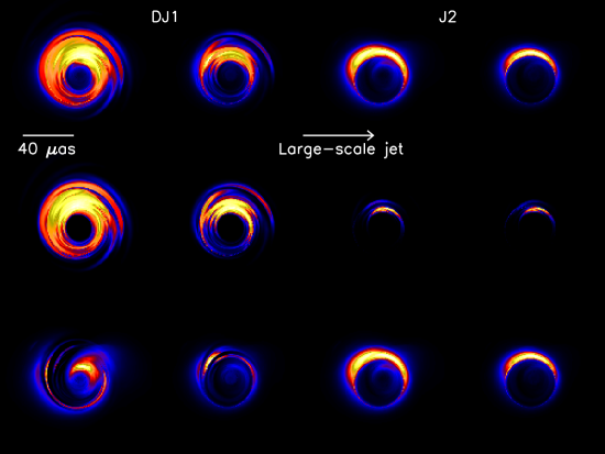
Figure 5: Images from total (top row), disc (middle row) and jet (bottom row) components for the two fiducial models (left two columns and right two columns) at $1.3$ mm (first and third columns) and $0.87$ mm (second and fourth columns). The colours are scaled linearly from blue to red to yellow to white, with a dynamic range of 60. The panel size is $100\times 100\mu$as. The images are taken from the same time step used for the spectra in Figure 4, and have been rotated $90^{\circ}$ to roughly align with the position angle of the large-scale jet at $7$ mm. Both fiducial model images are crescents from the combined effects of light bending and Doppler beaming. The disc component of DJ1 is similar to previous models of Sgr A*. The jet component in J2 is dominated by the counter-jet, while in DJ1 the jet component comes from the forward jet since the counter-jet emission is absorbed by the disc.

4 Image Morphology

Images of the fiducial models as well as their jet and disc components from the time step of the MBD simulation used for spectral fitting are shown in Figure 5 at $1.3$ mm and $0.87$ mm, the two wavelengths of interest for mm-VLBI. The orientation angle of the M87 black hole spin axis projected on the plane of the sky can be reasonably assumed to align with the orientation of the $7$ mm jet structure. This assumes that the jet is launched along the spin axis, and that the jet remains coherent on parsec scales. The images in Figure 5 have all been rotated to this favored orientation.

Images of M87 dominated by thermal particles in the accretion flow (DJ1) are nearly identical to those of Sgr A* (cf. Figure 11 of Dexter et al., 2010). Doppler beaming from the Keplerian velocity profile is significant even at the low expected inclination of M87 ($i=25^{\circ}$ here), but weaker than for preferred inclinations of Sgr A* ($\simeq 60^{\circ}$). The image is a crescent from the combined effects of beaming, light bending and gravitational lensing. The emission region is in the inner portion of the accretion flow ($r\sim 5M$) near the mid-plane (see Mościbrodzka et al., 2009; Dexter et al., 2010).

The jet emission arises from near the pole at very small radius ($r\sim 2-4M$), which falls mostly in the “shadow” region of the image, connected with an observer at infinity by photons that intersect the black hole. The portions outside the shadow for lines of sight at the low inclinations considered here ($i\lesssim 40^{\circ}$) are in the counter-jet rather than the forward jet. Inside the shadow, a small fraction of the emitted photons reach a distant observer, strongly suppressing the brightness of the forward jet. When the disc emission is negligible (J2), the lines of sight to the counter-jet are optically thin and the counter-jet dominates the jet image. The vertical velocity components are small at these small radii, so that the Doppler beaming is dominated by the azimuthal velocity component. This leads to the asymmetry in the jet component of the image. The jet image is still a crescent, although its intensity drops off sharply due to the strong radial dependence of the jet emissivity ($j_{\nu}\sim n_{\text{nth}}B^{2}\sim r^{-4}$ with $B\sim r^{-1}$ near the spectral peak). When the disc emission is significant, lines of sight to the counter-jet become optically thick, and the jet emission is dominated by the forward jet contribution (lower left two panels of Figure 5).

These are the first images of a jet launching region from a simulation. Images of the same time step are plotted in Figure 6 for inclinations of $90^{\circ}$ (edge-on, top left panel) to $0^{\circ}$ (face-on, bottom right panel) in even steps of $\cos{i}$, where $i$ is the inclination angle. For edge-on viewing, there is no distinction between jet and counter-jet and the image is split into two bright lobes close to the black hole. The image is highly asymmetric due to strong Doppler beaming from helical motion in the jet base. Moving to lower inclination, more and more of the forward jet falls into the shadow region where the path lengths are shorter and less of the orbital velocity is aligned with the line of sight. This causes the brightening of the counter-jet relative to the forward jet. At small inclinations, the forward jet is barely visible and the image is dominated by the counter-jet. This is the opposite of the behavior seen in extended jet emission where the material is ultra-relativistic and the radial velocity dominates. In that case, the forward- (counter-) jet is strongly Doppler boosted towards (away from) the observer at small inclinations. The counter-jet in M87 isn’t visible even on mas scales at $7$ mm. These jet images are also much different from those in Broderick & Loeb (2009), where the jet is launched farther from the black hole ($r\sim 10M$) than is found from the simulation assuming that $n_{\text{nth}}\propto b^{2}$. When the jet is launched farther from the black hole, the forward jet dominates the images at $1.3$ mm. For this reason, the jet images discussed here are sensitive to the uncertain mass loading in ultra-relativistic jets. Jet particle density profiles for M87 found from pair production calculations are qualitatively similar to those used here (Mościbrodzka et al., 2011).

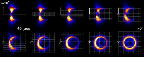
Figure 6: Jet images at observer inclinations ranging from edge-on (top left panel) to face-on (bottom right panel). The colours are scaled linearly from blue to red to yellow to white, with a dynamic range of 60. The panel size is $100\times 100\mu$as. The arrow shows the orientation of the black hole spin axis, and the grid is the xy-plane. For edge-on viewing there is strong asymmetry from Doppler boosting and no distinction between the jet/counter-jet, but as the inclination decreases the image becomes circularly symmetric and the counter-jet becomes more prominent as more of the forward jet emission is captured by the black hole.

In both the disc and jet models the circular photon orbit produces a black hole shadow at $1.3$ mm. At $0.87$ mm, both images are more compact. The jet component in DJ1 is less significant, and the J2 image is essentially just a single crescent from Doppler beaming of the jet material with a velocity component along the line of sight.

4.1 Predictions for mm-VLBI

The first mm-VLBI observations of M87 were conducted recently (Fish et al., 2011) using telescopes in Arizona, California, and Hawaii, but the results are not yet available. We therefore make predictions for both current and future telescopes, assuming a geometry (inclination and orientation) based on larger scale jet observations. With sufficient baseline coverage, sensitivity and observing time it may be possible to construct observational images in the future. However, for now the small number of available telescopes requires that models be fit to observations in the u-v plane. We Fourier transform the images to visibilities, whose amplitudes are shown along with the images for both mm-VLBI wavelengths in Figure 7. Possible locations of current measurements are shown as the green lines, and the visibility amplitudes are interpolated to those locations and plotted against baseline length in the top panel of Figure 8. In both fiducial models the current telescopes are at an orientation where the visibility amplitude decreases monotonically with baseline length. Fit with a symmetric Gaussian model, the source FWHM size is 43 (36) $\mu$as for this single time step of model DJ1 (J2).

However, the models are time variable and sensitive to the sky orientation. To make a more robust prediction, these effects are taken into account by fitting symmetric Gaussian models to visibilities from 120 images spaced evenly over the last $\simeq 2000$ M of simulation time ($\simeq 2$ years for M87) with sky orientations of $-75^{\circ}\pm 30^{\circ}$. In both models, the inferred source size increases with the total $1.3$ mm flux due to the emission region becoming optically thick. The inferred sizes ($\text{DJ1}_{\text{FWHM}}$ and $\text{J2}_{\text{FWHM}}$) can be expressed as power laws in flux as,

$$\text{DJ1}_{\text{FWHM}} \simeq (33\pm 6)\left(\frac{F_{\nu=230\text{GHz}}}{1\hskip 2.0pt\text{Jy}}\right)^{.5}\mu\text{as},$$ (11)

$$\text{J2}_{\text{FWHM}} \simeq (39\pm 8)\left(\frac{F_{\nu=230\text{GHz}}}{1\hskip 2.0pt\text{Jy}}\right)^{.25}\mu\text{as},$$ (12)

where the uncertainties are the 1$\sigma$ scatter both from the time variability and sky orientation. For the observed total flux of $1.77$Jy found by Tan et al. (2008), the predicted sizes are both $44\mu$as. VLBI observations of Sgr A* have found smaller fluxes on micro-arcsecond scales than those from single dish observations, in which case the values of $33\mu$as and $39\mu$as for $1$Jy may be more appropriate for M87.

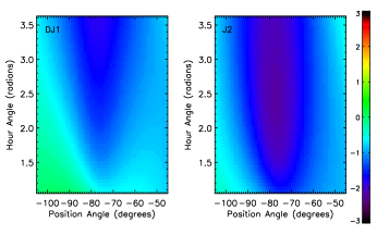
Figure 9: Predicted closure phase from the two fiducial models (left and right panels) at $1.3$ mm as functions of the position angle of the black hole spin axis and the projection of the Hawaii/California/Arizona baseline triangle on M87. For a large fraction of parameter space, the predicted closure phase differs significantly from zero, indicative of the asymmetric structure of the images.

We can also interpolate the visibilities from the fiducial models to the baselines probed by telescopes to be added to the mm-VLBI array in the near future in Chile and Mexico, and the results are shown in the bottom panel of Figure 8. In both cases, the black hole shadow is accessible to observations between Mexico and Hawaii. In the jet-dominated model, the shadow also appears on baselines between Chile and Mexico. Finally, the VLBI closure phase provides an additional constraint for any triangle of baselines, independent of that given by the visibility amplitude. Predicted closure phases for our two fiducial models as functions of position angle and the projection of the Hawaii/California/Arizona baseline triangle on M87 are shown in Figure 9. The predicted closure phase can deviate significantly from zero, indicative of asymmetric structure, especially in the jet-dominated model (J2). These results hold over the range of sky orientations and simulation time considered.

The maximum brightness temperatures, $kT_{b}=I_{\nu}c^{2}/2\nu^{2}$ in cgs units, where $I_{\nu}$ is the observed specific intensity, from the models are $3\times 10^{10}$ K (DJ1) and $7\times 10^{10}$ K (J2). The brightness temperature tracks the image intensity, and its maximum is larger for a more compact image. In the disc model, the maximum brightness temperature is in good agreement with the typical temperature of the electrons producing the millimetre emission.

5 Variability

As discussed above, these radiative disc/jet models of M87 are also time-dependent. Light curves from the fiducial models are shown in Figure 10 at $1.3$ mm and $0.87$ mm. The variability in the jet model is from one extended event, while the disc model light curve looks similar to that for the same simulation in the Sgr A* modeling (lower right panel of Figure 6 from Dexter et al., 2010). This disc variability is caused by fluctuations in the particle density and magnetic field strength driven by MRI turbulence, and are strongly correlated with the accretion rate. Both models are consistent with the finding that M87 varies at about $1\hskip 2.0pt\text{Jy}\hskip 2.0pt\text{yr}^{-1}$ (Steppe et al., 1988). However, longer light curves would be required to make a statistically significant statement about the variability. This is particularly true in the jet model, where the variability is the result of one event. It is unclear whether this is due to a transient effect in the jet formation/propagation or recurrent variable activity.

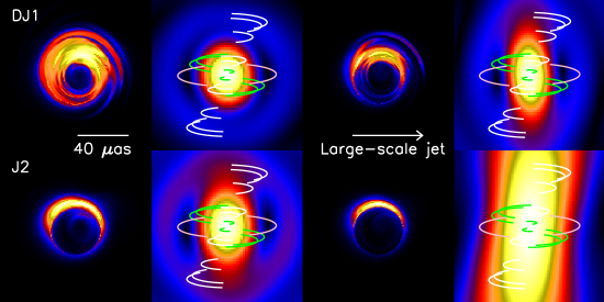
Figure 7: Images (first and third columns) and corresponding visibility amplitudes (second and fourth columns) from the two fiducial models (rows) at $1.3$ mm (first two columns) and $0.87$ mm (right two columns). The colours are scaled linearly from blue to red to yellow to white, with a dynamic range of 60. The panel size is $100\times 100\mu$as. The baseline orientations available to current (green) and near future (white and pink) telescopes are overplotted as lines. At this orientation, set by the direction of the $7$ mm jet, the black hole shadow is accessible to future observations on a Hawaii-Mexico baseline.

6 Discussion

We have created the first radiative disc/jet models of M87 based on GRMHD simulations. The jet is formed, collimated and accelerated self-consistently from an accretion flow within the ideal MHD approximation and the limitations of the numerical scheme. The disc/jet boundary is taken as a contour in the ratio of magnetic to rest mass energy density or in the particle specific enthalpy as measured at infinity, with similar results in either case. The disc portion is modeled as thermal electrons with a constant ion-electron temperature ratio as in previous models of Sgr A*, while the internal energy of the power law electrons in the jet region is scaled as a fixed fraction of the magnetic energy density. The emission mechanism is synchrotron radiation in both cases. Two separate types of models can describe the high resolution spectrum of M87. In one class of models, the disc emission is negligible at all frequencies and the jet produces the entire spectrum. In the other, the jet produces the low and high frequency spectrum, while the millimetre emission is produced by thermal disc electrons.

6.1 Favored Parameter Values

The favored jet parameter combinations are $\gamma_{\text{min}}=30-100$, $p=3.25-3.5$ and $\eta=0.02-0.10$. The favored average accretion rate is $\dot{m}=(1-2)\times 10^{-4}$, or $\dot{M}=(1-2)\times 10^{-3}M_{\odot}\text{yr}^{-1}$. For the jet portion, the parameters $\dot{m}$, $\eta$ and $\gamma_{\text{min}}$ are partially degenerate. Ignoring important effects of optical depth and the cutoff frequency on the spectrum, $F_{\nu_{\text{max}}}\sim\eta\dot{M}^{2}\gamma_{\text{min}}^{4}$, while $\nu_{\text{max}}\propto\sqrt{\dot{m}}\gamma_{\text{min}}^{2}$. Jet spectra with $\gamma_{\text{min}}=1000$ peak in the near-IR or optical, inconsistent with VLBI observations of extended jet emission in the radio. Smaller $\dot{m}$ is required at larger $\gamma_{\text{min}}$ to keep the spectral peak in the millimetre. The fraction of magnetic energy density in non-thermal electrons, $\eta$, can be used to scale to the correct normalization for any $\gamma_{\text{min}}$ and $\dot{m}$ as long as it remains less than unity and small enough so that the jet remains magnetically dominated (Equation 10). The spectral slope, $p$, is fixed by the near IR and optical observations, while the ion-electron temperature ratio $T_{i}/T_{e}$ determines whether the disc or jet produces the emission at millimetre wavelengths. The favored value for this simulation from Sgr A* models, $T_{i}/T_{e}=3$ (Dexter et al., 2010), leads to a disc-dominated millimetre image.

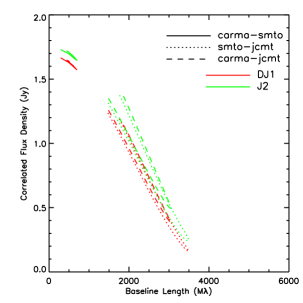
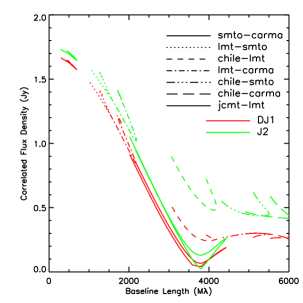
Figure 8: Model visibility amplitude vs. baseline length for current (top) and near future (bottom) telescopes. The visibility amplitude falls off monotonically with baseline length for current measurements and can be fit reasonably well with a circular Gaussian model. The black hole shadow appears as a local minimum in the visibility profile, and is accessible to a future baseline between Hawaii and Mexico.

6.2 Radiative Efficiency

By ignoring radiation in the simulations, we have assumed that the accretion flow is radiatively inefficient. We can check this assumption by calculating the radiative efficiency, $\epsilon=L/\dot{M}c^{2}$, where $L\sim 2\times 10^{42}\hskip 2.0pt\text{erg}\hskip 2.0pt\text{s}^{-1}$ is the bolometric luminosity of the models. This gives $\epsilon\sim(1-4)\times 10^{-2}$, so that the radiative models are radiatively inefficient and marginally self-consistent. The effects of radiative cooling on the dynamical solution should be considered in future simulations. Using axisymmetric GRMHD simulations, Mościbrodzka et al. (2011) found lower accretion rates, $\dot{M}\simeq 10^{-4}M_{\odot}\text{yr}^{-1}$, and larger bolometric luminosities, $L\sim 10^{44}\hskip 2.0pt\text{erg}\hskip 2.0pt\text{s}^{-1}$, leading to unphysically large radiative efficiencies ($\simeq 16$, see their Table 1). Their models used a smaller black hole mass and $T_{i}=T_{e}$, which together could explain the small accretion rates found. The bolometric synchrotron luminosity $L\sim nB^{2}T_{e}^{2}M^{3}\propto\dot{M}^{2}T_{e}^{2}/M^{3}$. Using the factor $\simeq 2.1$ smaller black hole mass and factor of $2$ larger electron temperature then requires an order of magnitude decrease in accretion rate to produce the observed flux, which explains the difference. Their models also include Compton scattering, which is neglected here. Extending our non-thermal jet spectrum to the X-ray does not significantly change its bolometric luminosity, but including Compton scattering would both increase the bolometric luminosity and allow us to include a constraint from the observed X-ray luminosity (Wilson & Yang, 2002). In Mościbrodzka et al. (2011), the spectral energy distribution from the simulation without radiative cooling peaks at $\nu\gtrsim 10^{20}$Hz. It is unclear whether Compton scattering would have such an important effect if included in our 3D models.

We can crudely estimate the relative significance of Compton scattering for both models. In the jet model, the ratio of peak $\nu F_{\nu}$ for synchrotron and self-Compton components in a homogeneous blob with a power law distribution of electrons, ignoring all relativistic and viewing effects is (e.g., Sari & Esin, 2001):

$$\frac{\nu F_{\nu}(\text{IC})}{\nu F_{\nu}(\text{Syn})}\sim\frac{2}{3}\frac{p-1}{p+3}\sigma_{T}\hskip 2.0ptn\hskip 2.0ptR\hskip 2.0pt\gamma_{\text{min}}^{p-1}\hskip 2.0pt\gamma_{\text{max}}^{3-p},$$ (13)

where $\sigma_{T}$ is the Thompson cross-section and $R$ is the size of the emitting blob. Scaling to reasonable parameters for our jet model gives,

$$\frac{\nu F_{\nu}(\text{IC})}{\nu F_{\nu}(\text{Syn})}\sim 0.5\left(\frac{R}{5M}\right)\left(\frac{n}{10^{7}\hskip 2.0pt\text{cm}^{-3}}\right)\left(\frac{\gamma_{\text{min}}}{50}\right)^{5/2}\left(\frac{\gamma_{\text{max}}}{10^{5}}\right)^{-1/2}.$$ (14)

This estimate is not self-consistent. We have scaled the electron number density to the typical value for thermal disc electrons which provide the scattering optical depth, but then assumed they have a power law energy distribution. This is a conservative approach, since thermal electrons would have a much sharper high energy cutoff.

For the disc model, we use the approximate local prescription given in Esin et al. (1996) to calculate the Comptonization enhancement to the bolometric thermal synchrotron luminosity. This enhancement depends sensitively on the scattering optical depth and weakly on the seed photon energy. The scattering optical depth is taken to be $\tau=n\sigma H$, where $\sigma$ is the Thomson scattering cross section and $H\equiv(H/R)R$ is the disc height, where $H/R\simeq 0.2$ for the simulation considered here. Comptonization is estimated from the peak frequency of the synchrotron spectrum, $\nu_{p}\sim 10^{11-12}$Hz for the disc models. The estimate is mostly independent of $\nu_{p}$ within this range. Using typical values of $n=10^{7}\hskip 2.0pt\text{cm}^{-3}$, $R=1$ M, and $T=2\times 10^{10}$ K, we find the relative Compton luminosity $L_{\text{IC}}/L_{\text{Syn}}\simeq 1$. Numerically integrating the Compton cooling rate over the simulation domain gives a similar answer. However, this enhancement factor is extremely sensitive to the assumed scattering optical depth. For example, replacing the disc height $H$ with radius $R$ in the expression above gives $L_{C}/L_{S}\sim 10$, or a radiative efficiency $\epsilon\lesssim 1$, invalidating our assumption that radiation can be added after the fact without changing the (thermo)dynamics of the accretion flow.

From both estimates, it is clear that Compton scattering is an important mechanism and will significantly affect the observed X-ray emission. However, we estimate that it may only lead to an order unity correction in the bolometric luminosity of both of our models. Including optically thin synchrotron and Compton cooling self-consistently is an important goal for future simulations of M87, and may significantly affect the resulting radiative model. However, this is complicated by the uncertain ion-electron coupling. Including optically thin radiative cooling in standard single fluid simulations assumes perfect coupling between the ions and electrons, since both species are cooled equally.

For completeness, we can also estimate the bolometric luminosity from bremsstrahlung:

$$L_{B}\sim 10^{40}\left(\frac{n}{10^{7}\hskip 2.0pt\text{cm}^{-3}}\right)^{2}\left(\frac{T}{10^{10}\hskip 2.0pt\text{K}}\right)^{1/2}\left(\frac{R}{10M}\right)^{3}\text{erg}\hskip 2.0pt\text{s}^{-1},$$ (15)

a few orders of magnitude less than the synchrotron luminosity. Including the large-scale accretion flow, with much smaller particle densities and temperatures but a much larger volume, will increase this estimate and both Compton scattering and bremsstrahlung could be important emission mechanisms at X-ray energies.

6.3 Images

Assuming that the M87 jet propagates along the black hole spin axis, its orientation angle is constrained to be roughly $-75\pm 30^{\circ}$ measured E of N. The inclination has been estimated to be $\simeq 25^{\circ}$ from the Lorentz factor of the jet (Heinz & Begelman, 1997; Biretta, Sparks & Macchetto, 1999). For these parameters, we can make predictions for ongoing mm-VLBI observations. On current baselines, we predict that M87 should appear as a compact source similar to Sgr A*. The fiducial models have FWHM sizes of $22-68$$\mu$as when fit with symmetric Gaussian models over the entire range of sky orientations and simulation time steps considered. For reasonable values of the total $1.3$ mm flux, the sizes are largely in the range $33-44\mu$as, similar to the size of $37\mu$as found in the first mm-VLBI observations of Sgr A* (Doeleman et al., 2008).

The black hole shadow is accessible to future observations on baselines between Mexico and Hawaii and possibly Mexico and Chile. Although the predicted Gaussian sizes for current telescopes are nearly identical for both fiducial models, future observations with additional telescopes or epochs should be able to distinguish between the two. This is because the 2D structure of the images is significantly different and future baselines will probe orientations where the predictions differ substantially. Future mm-VLBI observations will also measure polarized emission on event horizon scales, and including polarization in the radiative transfer calculations is a goal for future work.

Both images are crescents, as in the case of Sgr A*. When the emission region is compact enough and the velocities are roughly Keplerian disc motion and helical jet motion, the resulting image is a crescent, qualitatively independent of the details of the physics in the innermost part of the accretion flow. The sky orientation (position angle) determines the orientations measured by VLBI. Thus, our predictions for mm-VLBI with current and future telescopes are fairly robust as long as the assumed geometry is accurate and the millimetre emission region is compact ($r\lesssim 10$ M), despite the fact that the fiducial models chosen here are only representative of a range of possibilities for explaining the spectral properties of M87. The compactness requirement for the emission region is equivalent to assuming a steeply declining emissivity with radius, and a small optical depth ($\tau\lesssim 1$) to the emission region.

At inclinations of $10^{\circ}$ ($40^{\circ}$), the images become less (more) Gaussian and more (less) circular. The crescent morphology and size predictions are less sensitive to changes in inclination within this range than to uncertainties in the model (DJ1 or J2) or position angle.

We have assumed the new mass estimate of $6.4\times 10^{9}M_{\odot}$ (Gebhardt & Thomas, 2009; Gebhardt et al., 2011) throughout. Changing the black hole mass changes the favored parameter values, but does not substantively change the types of feasible models or other major results. The exception is in the size predictions for mm-VLBI, which essentially scale with mass. If the black hole mass in M87 is $3\times 10^{9}M_{\odot}$ (Marconi et al., 1997), then the predicted sizes would be a factor $\simeq 2$ smaller. This means that mm-VLBI can provide a model-dependent test of the black hole mass – if a size smaller than $\simeq 22\mu$as is found, the smallest for our models over the range of simulation time and valid position angles, it may indicate a smaller black hole mass. Conversely, a relatively large measured size would favor the larger black hole mass estimate, although it could also mean that the emission at $1.3$ mm is more extended than found from current GRMHD simulations.

Figure 10: Light curves from the two fiducial models (left and right panels) at $1.3$ mm (top row) and $0.87$ mm (bottom row). The disc variability is driven by MRI turbulence, as previously found in similar models of Sgr A* (Dexter, Agol & Fragile, 2009; Dexter et al., 2010).

6.4 Uncertainties

There are many uncertainties in this analysis. The assumption that the internal energy in non-thermal particles scales with magnetic field energy density may be reasonable (e.g., Broderick & McKinney, 2010), but it is made out of necessity. Both the internal energy (pressure) and mass density from the simulation are set by the artificial numerical floor required for code stability when $b^{2}/\rho c^{2}\gg 1$, the region of interest for jet launching. Radiation is added in post-processing, despite the fact that the models are found to be marginally radiatively efficient. Both synchrotron and Compton scattering have been found to be dynamically important in axisymmetric simulations of M87 (Mościbrodzka et al., 2011) with similar parameters to our disc/jet model (DJ1). It will be possible to include those forms of cooling in future simulations, but a method for evolving the non-thermal particle density self-consistently is much more difficult.

Previous semi-analytic disc/jet models of M87 have invoked a truncated disc, with a low, constant particle density and magnetic field strength throughout the inner disc. This configuration can produce the observed radio emission. We find that the magnetic field strength in MBD and other GRMHD simulations falls off with radius ($\propto r^{-1.2}$ for MBD). Producing the observed flux then requires that the disc emission peaks at millimetre wavelengths. Although none of our models can explain the observed radio emission, the agreement is much better if the models are fit to only the unresolved emission from the core of radio images (cf. Reynolds et al., 1996; Di Matteo et al., 2003).

Both the disc and jet models used here are unlikely to be valid outside the innermost radii. The accretion flow solution is probably reliable only out to $r\simeq 10$ M, but the disc emission region is so compact that this does not affect the results. However, there are so few studies of jets launched from GRMHD simulations that it is unclear what the domain of validity is. This situation will improve in the near future, as numerical techniques for propagating large-scale jets improve and simulations are able to be evolved for longer physical times due to the increase in available computational resources. The jet solution in a new simulation similar to MBD but with much higher resolution (272$\times$128$\times$256), a larger radial boundary ($26000$ M) and a longer duration ($20000$ M) is nearly identical to that of MBD within $r\lesssim 8$ M ($B\propto r^{-1}$), but has a nearly flat radial magnetic field strength profile outside of that. Preliminary images based on a single time step from this simulation display extended (mas) structure in the radio, but give nearly identical predictions for mm-VLBI of M87, indicating that the low resolution used in MBD is unlikely to invalidate the results of this paper. Models from this and other high resolution, geometrically thick simulations (McKinney, Tchekhovskoy & Blandford, 2012) will be considered in a subsequent publication.

7 Summary

We have constructed the first radiative disc/jet models of M87 based on a general relativistic MHD simulation of a black hole accretion flow. The main results of this study are:

1. The spectral energy distribution of the core of M87 can be explained with jet or disc/jet models.

2. In both types of models the images at $1.3$ mm are crescents from the combination of gravitational lensing and Doppler beaming of the compact emission region.

3. The jet emission is produced in the counter-jet near the pole in the immediate vicinity of the black hole ($r\lesssim 4$ M), while the disc emission is produced near the midplane in the inner radii $r\simeq 5$ M as found in previous models of Sgr A*.

4. For the favored viewing geometry of M87 based on analyses of the large-scale jet, we predict a Gaussian source structure with a size of $33-44\mu$as ($\simeq 5$ Schwarzschild radii) for observations with current mm-VLBI telescopes. The inferred size should increase slowly with increasing flux. The black hole shadow, direct evidence for an event horizon, may be detected on future baselines between Hawaii (JCMT) and Chile (ALMA/APEX/ASTE).

5. The two types of models can be distinguished with mm-VLBI observations on baselines including telescopes in Mexico (LMT) and Chile (ALMA/APEX/ASTE), or by measuring the change in size between epochs of different total $1.3$ mm flux.

References

- Baath et al. (1992) Baath L. B. et al., 1992, A&A, 257, 31
- Bardeen (1973) Bardeen J. M., 1973, in Black holes (Les astres occlus), DeWitt B. S., DeWitt C., eds., New York: Gordon and Breach, p. 215
- Biretta, Sparks & Macchetto (1999) Biretta J. A., Sparks W. B., Macchetto F., 1999, ApJ, 520, 621
- Broderick (2006) Broderick A. E., 2006, MNRAS, 366, L10
- Broderick et al. (2011) Broderick A. E., Fish V. L., Doeleman S. S., Loeb A., 2011, ApJ, 735, 110
- Broderick & Loeb (2009) Broderick A. E., Loeb A., 2009, ApJ, 697, 1164
- Broderick & McKinney (2010) Broderick A. E., McKinney J. C., 2010, ApJ, 725, 750
- De Villiers et al. (2005) De Villiers J.-P., Hawley J. F., Krolik J. H., Hirose S., 2005, ApJ, 620, 878
- Dexter (2011) Dexter J., 2011, PhD thesis, University of Washington
- Dexter & Agol (2009) Dexter J., Agol E., 2009, ApJ, 696, 1616
- Dexter, Agol & Fragile (2009) Dexter J., Agol E., Fragile P. C., 2009, ApJ, 703, L142
- Dexter et al. (2010) Dexter J., Agol E., Fragile P. C., McKinney J. C., 2010, ApJ, 717, 1092
- Di Matteo et al. (2003) Di Matteo T., Allen S. W., Fabian A. C., Wilson A. S., Young A. J., 2003, ApJ, 582, 133
- Doeleman et al. (2008) Doeleman S. S. et al., 2008, Nature, 455, 78
- Esin et al. (1996) Esin A. A., Narayan R., Ostriker E., Yi I., 1996, ApJ, 465, 312
- Falcke, Melia & Agol (2000) Falcke H., Melia F., Agol E., 2000, ApJ, 528, L13
- Fish et al. (2011) Fish V. L. et al., 2011, ApJ, 727, L36+
- Fragile et al. (2007) Fragile P. C., Blaes O. M., Anninos P., Salmonson J. D., 2007, ApJ, 668, 417
- Fuerst & Wu (2004) Fuerst S. V., Wu K., 2004, A&A, 424, 733
- Gammie, McKinney & Tóth (2003) Gammie C. F., McKinney J. C., Tóth G., 2003, ApJ, 589, 444
- Gebhardt et al. (2011) Gebhardt K., Adams J., Richstone D., Lauer T. R., Faber S. M., Gültekin K., Murphy J., Tremaine S., 2011, ApJ, 729, 119
- Gebhardt & Thomas (2009) Gebhardt K., Thomas J., 2009, ApJ, 700, 1690
- Goldston, Quataert & Igumenshchev (2005) Goldston J. E., Quataert E., Igumenshchev I. V., 2005, ApJ, 621, 785
- Gracia et al. (2009) Gracia J., Vlahakis N., Agudo I., Tsinganos K., Bogovalov S. V., 2009, ApJ, 695, 503
- Hada et al. (2011) Hada K., Doi A., Kino M., Nagai H., Hagiwara Y., Kawaguchi N., 2011, Nature, 477, 185
- Heinz & Begelman (1997) Heinz S., Begelman M. C., 1997, ApJ, 490, 653
- Hilburn & Liang (2011) Hilburn G., Liang E., 2011, ArXiv e-prints
- Junor, Biretta & Livio (1999) Junor W., Biretta J. A., Livio M., 1999, Nature, 401, 891
- Legg & Westfold (1968) Legg M. P. C., Westfold K. C., 1968, ApJ, 154, 499
- Leung, Gammie & Noble (2011) Leung P. K., Gammie C. F., Noble S. C., 2011, ApJ, 737, 21
- Ly, Walker & Wrobel (2004) Ly C., Walker R. C., Wrobel J. M., 2004, AJ, 127, 119
- Marconi et al. (1997) Marconi A., Axon D. J., Macchetto F. D., Capetti A., Sparks W. B., Crane P., 1997, MNRAS, 289, L21
- McKinney (2006a) McKinney J. C., 2006a, MNRAS, 367, 1797
- McKinney (2006b) —, 2006b, MNRAS, 368, 1561