Large-Scale High-Lundquist Number Reduced MHD Simulations of the Solar Corona Using GPU Accelerated Machines

Abstract

We have recently carried out a computational campaign to investigate a model of coronal heating in three-dimensions using reduced magnetohydrodynamics (RMHD). Our code is built on a conventional scheme using the pseudo-spectral method, and is parallelized using MPI. The current investigation requires very long time integrations using high Lundquist numbers, where the formation of very fine current layers challenge the resolutions achievable even on massively parallel machines. We present here results of a port to Nvidia CUDA (Compute Unified Device Architecture) for hardware acceleration using graphics processing units (GPUs). In addition to a brief discussion of our general strategy, we will report code performance on several machines which span a variety of hardware configurations and capabilities. These include a desktop workstation with commodity hardware, a dedicated research workstation equipped with four Nvidia C2050 GPUs, as well as several large-scale GPU accelerated distributed memory machines: Lincoln/NCSA, Dirac/NERSC, and Keeneland/NICS.

¹Space Science Center, University of New Hampshire, Durham, NH 03824

²Geophysical Institute, University of Alaska Fairbanks, Fairbanks, AK 99775

1 Introduction

The Reduced Magnetohydrodynamics Coronal Tectonics code (RMCT) solves the reduced MHD equations in three dimensions using a standard pseudo-spectral semi-implicit scheme and predictor-corrector time stepping. The code has been tailored for studying the role of magnetic reconnection and singular current layers in the heating of the solar corona. Within the framework of Parker’s model of coronal heating (Parker 1972), a recent analysis in two dimensions (Ng & Bhattacharjee 2008) demonstrated that when coherence times ($\tau_{coh}$) of imposed photospheric turbulence are much smaller than characteristic resistive time-scales ($\tau_{R}$), the Ohmic dissipation scales independently of resistivity. While their initial 2-D RMHD treatment precluded non-linear effects such as instabilities and/or magnetic reconnection they further invoked a simple analytical argument that demonstrated that even considering these non-linear effects which would limit the growth of $B_{\perp}$, given small enough $\tau_{coh}$, the same insensitivity to resistivity would be recovered. The RMCT code has been used in a computational campaign to extend this analysis to three dimensions (Ng et al. 2011). Spanning three orders of magnitude in Lundquist number, this campaign requires very high resolution to correctly resolve dissipative MHD structures, and very long time integrations to obtain adequate statistics. The high Lundquist number limit has proved particularly challenging even when parallelized on distributed memory machines. In this paper we present a comprehensive reprogramming of our RMHD code for hardware acceleration using general purpose graphics processing units (GPUs).

Recent years have seen the rapid emergence of graphics processing units as hardware accelerators for general purpose computation and high performance computing. Computational scientists have benefited from GPUs in fields as diverse as geology, molecular biology, weather prediction, high energy nuclear physics (lattice QCD), quantum chemistry, finance and oil exploration.

In computational plasma astrophysics, several groups have reported progress using GPU acceleration for magnetohydrodynamics (MHD) (Wong et al. 2009; Wang et al. 2010; Zink 2011), astrophysical gyro-kinetics (Madduri et al. 2011), and particle-in-cell simulations (Stantchev et al. 2008).

The work we describe here is most similar to that of Stantchev et al. (2009). Using a G80 generation (128 stream processors single precision) NVidia GPU, compared with a single 3.0 GHz Intel Xeon using $1024^{2}$ perpendicular resolution, they report a up to a $14\times$ speedup for a Hasegawa-Mima equation solver and 25-30$\times$ speedup for a pseudo-spectral RMHD code in single precision. We describe in this paper a full fledged three dimensional reduced MHD production code and report code performance using the latest generation Nvidia GPUs on GPU equipped workstations as well as several distributed memory GPU accelerated machines.

2 Reduced Magnetohydrodynamics and the Parallel Numerical Scheme

The RMHD equations are a simplified version of MHD applicable to systems where the plasma is dominated by a strong guide field such that the timescales of interest are slow compared with the characteristic Alfvén timescale $\tau_{A}$. These restrictions also imply incompressibility ($\nabla\cdot V=0$) and the exclusion of magnetosonic modes (leaving only the shear Alfvén modes propagating in $\hat{e}_{z}$). The RMHD equations were first derived for the study of tokamak plasmas by Kadomtsev & Pogutse (1974) and Strauss (1976), which can be written in dimensionless form as

$$\frac{\partial\Omega}{\partial t}+[\phi,\Omega]=\frac{\partial J}{\partial z}+[A,J]+\nu\nabla^{2}_{\perp}\Omega,$$ (1)

$$\frac{\partial A}{\partial t}+[\phi,A]=\frac{\partial\phi}{\partial z}+\eta\nabla^{2}_{\perp}A,$$ (2)

where $A$ is the flux function so that the magnetic field is expressed as $\mathbf{B=\mathbf{\hat{e_{z}}}+B_{\perp}}=\mathbf{\hat{e_{z}}}+\nabla_{\perp}A\times\mathbf{\hat{e_{z}}}$; $\phi$ is the stream function so that the fluid velocity field is expressed as $\mathbf{v}=\nabla_{\perp}\phi\times\mathbf{\hat{e_{z}}}$; $\Omega=-\nabla^{2}_{\perp}\phi$ is the $z$-component of the vorticity; $J=-\nabla^{2}_{\perp}A$ is the $z$-component of the current density; and the bracketed terms are Poisson brackets such that, for example, $[\phi,A]\equiv\phi_{y}A_{x}-\phi_{x}A_{y}$ with subscripts here denoting partial derivatives. The normalized viscosity $\nu$ is the inverse of the Reynolds number ${\sf{R_{v}}}$, and resistivity $\eta$ is the inverse of the Lundquist number $S$. The normalization adopted in equations (1) and (2) is such that the magnetic field is in the unit of $B_{z}$ (assumed to be a constant in RMHD); velocity is in the unit of $v_{A}=B_{z}/(4\pi\rho)^{1/2}$ with a constant density $\rho$; length is in the unit of the transverse length scale $L_{\perp}$; time $t$ is in the unit of $L_{\perp}/v_{A}$; $\eta$ is in the unit of $4\pi v_{A}L_{\perp}/c^{2}$; and $\nu$ is in the unit of $\rho v_{A}L_{\perp}$.

The numerical scheme we employ in this work was adapted from Longcope & Sudan (1994) and Longcope (1993). The simulation domain is a rectangular cartesian box of ($L_{z}\times L_{\perp}\times L_{\perp}$), permeated by guide-field $B_{z}$ line-tied at both ends representing the photosphere. Time integration is performed with a second order predictor corrector method. Perpendicular dimensions are bi-periodic for a pseudo-spectral scheme using standard two-thirds rule de-aliasing and in the parallel dimension a second order finite difference method is used. The original was written in Fortran90 and parallelization is accomplished by domain decomposition in $\hat{e}_{z}$ using MPI. Typical resolutions used for our coronal heating scaling study range from $64^{2}\times 32$ up to $1024^{2}\times 128$ and as with many pseudo-spectral schemes, the 2D FFTs dominate the computational burden typically consuming more than $80\%$ of computation time for the resolutions we target.

3 Numerical Results on Parker’s Model of Coronal Heating

It is crucial to the scaling study that we obtain good statistics averaging over time evolution in statistical steady state. As with previous long time integration studies of the Parker model, the runs are started with a vacuum potential field. After a time of the order of the resistive diffusion time, the system will evolve to a statistical steady state.

The range of $\eta$ has been extended to lower values (with $\tau_{c}=10\ll\tau_{r}$) for about an order of magnitude as compared with the study in (Longcope & Sudan 1994) which stopped at $\eta\sim 10^{-3}$. This extension of course requires significant increase in resolution, with our highest resolution case at $512^{2}\times 64$ so far, as compared with $48^{2}\times 10$ in (Longcope & Sudan 1994). The main difficulty in performing these simulations is the requirement to run up to hundreds or even thousands of Alfvén times in order to obtain good statistics of the average quantities under the driving of random boundary flow.

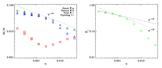
Figure 1.: (a) Average energy dissipation rate for different values of $\eta$. $\triangle$ is Ohmic dissipation, $\Box$ is viscous dissipation, $\Diamond$ is the total of the two, and $\bigcirc$ is the footpoint Poynting flux. (b) Average perpendicular magnetic field strength for different values of $\eta$.

Fig. 1 shows some of the scaling results we obtained so far. In Fig. 1 (a), the time-averaged Ohmic dissipation rate $\bar{W}_{\eta}$ (at the saturated level) for different $\eta$ is plotted in triangles, while the viscous dissipation rate $\bar{W}_{\nu}$ are plotted in squares. Note that $\bar{W}_{\nu}\ll\bar{W}_{\eta}$ in general. The time-averaged Poynting flux $\bar{I}$ is also plotted in the same graph in circles. It is supposed to be of the same value as $\bar{W}$ theoretically, and we do see that the differences between these two quantities are generally small in our numerical results, indicating acceptable accuracy.

Due to the fact that we are doing 3D simulations, and that we need to simulate for a long time to obtain good statistics, so far we have only been able to extend the value of $\eta$ to about an order of magnitude lower, as compared with similar studies in (Longcope & Sudan 1994). Nevertheless, we can see already that below $\eta\sim 10^{-3}$, there is a significant deviation from the scalings obtained in (Longcope & Sudan 1994), who showed by numerical results and scaling analysis that both $\bar{W}$ and $\bar{B_{\perp}}$ should scale with $\eta^{-1/3}$ in the small $\eta$ limit. We have added dotted lines in Fig. 1 (a) and (b) showing the $\eta^{-1/3}$ scaling. For more details of these numerical results, as well as an analysis showing the transition of scaling behavior from (Longcope & Sudan 1994) to ours, please see (Ng et al. 2011).

4 GPU implementation

CUDA is a parallel computing engine developed specifically for general purpose applications using NVidia GPUs. It allows programmers to leverage the high-throughput power of GPUs by programming in the familiar ANSI C language rather than resorting to reverse engineering native graphics languages (such as Open GL or Cg) to perform general purpose and scientific computations. The CUDA model allows programmers to delegate serial tasks required by the CPU by usual C code while extensions to C are provided for programming GPUs to exploit data parallelism. CUDA (now version 4.0 as of this writing) provides libraries for basic linear algebra (CUBLAS), sparse matrices (CUSPARSE), random number generation (CURAND), standard templates (THRUST), and fast Fourier transforms (CUFFT) as well as tools for profiling (Compute Visual Profiler) and debugging (CUDA-gdb). In the present study, we follow Stantchev et al. (2009) (and most all the studies mentioned previously) in adopting CUDA for our acceleration project.

Name	CPU	Nodes	GPUs	Network
Carver/NERSC	Nehalem(8 core)2.67 Ghz	400	None	QDR
Lincoln/NCSA	Harpertown(4 core)2.33Ghz	192	96 x S2070	SDR
Dirac/NERSC	Nehalem(8 core)2.67 Ghz	44	44 x C2050	QDR
UAF Workstation	Gulftown(12 core)2.8 Ghz	1	4 x C2050	-
Keeneland/NICS	Westmere(6 core)2.67 Ghz	120	360 x C2070	QDR

Table 1.: Specifications for Carver/NERSC and several GPU accelerated machines.

Our strategy for a comprehensive reprogramming of RMCT for GPU acceleration with CUDA can be summarized as follows: $\mathbf{[1]}$ Perform FFTs using the CUFFT library. The library is about an order of magnitude faster than our original FFT implementation when not considering CPU-GPU memory transfers but only several times faster when including them. We aim therefore to maximize the number of FFTs per memory transfer, and to perform intermediary tasks on the GPU. $\mathbf{[2]}$ Recycle memory of intermediate quantities. There is limited memory available on the GPU board so one must adequately budget memory allocated on board in such a manner as to observe $\mathbf{[1]}$. $\mathbf{[3]}$ Write simple kernels for point-wise arithmetic. Point-wise arithmetic is the bread and butter of stencil-operation based MHD codes, and CUDA implementations of such codes have been published (Wong et al. (2009) Wang et al. (2010) and Zink (2011)). It is tempting to say that such operations take a back seat in the current pseudo-spectral application to FFTs, but as we have seen Amdahl’s law would require that these kernels also see full consideration. $\mathbf{[4]}$ Preserve the underlying MPI decomposition. We are dealing here with two levels of parallelization, the first being the domain decomposition in $z$ and the second being the massive parallelism afforded by GPUs. The wide availability of multi-GPU workstations and GPU accelerated distributed memory machines warrants the pursuit of both parallelization methods in tandem. For this code, we pair one CPU core to one GPU, each core responsible for one sub-cube in the the $z$ domain decomposition scheme.

5 GPU Code Performance and Discussion

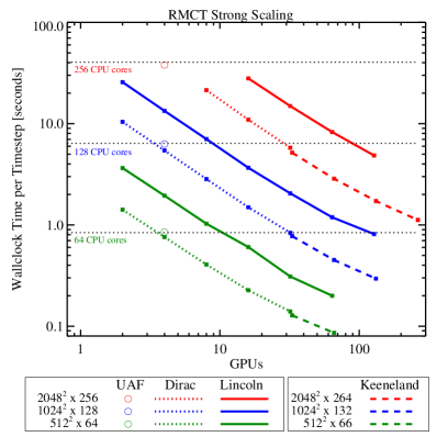
Figure 2.: Strong scaling of RMCT CUDA on various large scale distributed memory machines.

Figure 2 shows scaling results for RMCT CUDA on several GPU accelerated distributed memory machines. Measurements were made for each of five machines whose relevant specifications are summarized in Table 1. For a base-line comparison we use Carver, an IBM iDataplex mid-sized traditional CPU cluster at the National Energy Research Scientific Computing Center (NERSC) on which we have achieved the best performance thus far with the original version of the code. Carver hosts a GPU testbed cluster named Dirac which accelerates each of 44 nodes with a single NVidia C2050 GPU. A larger dedicated GPU production cluster at the National Center for Supercomputing Applications (NCSA) was available through TeraGrid, and paired 96 S2070s (4 GT200 GPU module) with 192 nodes. A dedicated GPU accelerated desktop workstation was acquired for this project and is running at the University of Alaska Fairbanks with four C2050 GPUs. The most powerful machine on which we have tested is the Keeneland Initial Delivery System hosted at the National Institute for Computational Science (NICS) and Georgia Tech. It features 120 nodes each accelerated by 3 C2070s, and is to be expanded to a full production system for TeraGrid (now called XSEDE) using next generation NVidia GPUs in the coming year.

As the codes currently stand, the CUDA port on Lincoln/NCSA at full scale is able to achieve roughly an order of magnitude speedup compared with Carver. Considering the performance of the code on the UAF workstation, the chip-to-chip equivalence is roughly 4, 8, and 16. As expected, the possibility of exposing maximal fine-grained parallelism given finer grids improves the potential for increasing this equivalence ratio. Actually observing an increase in this ratio then attests to the quality of the re-coding effort. At full scale on Keeneland, using the Fermi class GPUs the code is able to achieve up to a $30\times$ speedup beyond what was previously achieved on Carver.

The principal caveat of the present analysis is that we have spent much of our time optimizing the CUDA port, and have used as a basis of comparison, an original Fortran/MPI code which remains largely the same. The results reported here therefore should be taken as an effective speedup for a small academic coding team (consisting of a professor and graduate student) going from one practically deployable code to another.

Acknowledgments

Computer time was provided by UNH (using the Zaphod Beowulf cluster at the Institute for the Study of Earth, Oceans and Space), as well as a grant of HPC resources from the Arctic Region Supercomputing Center and the DoD High Performance Computing Modernization Program. This work is supported by NASA grants NNX08BA71G, NNX06AC19G, a NSF grant AGS-0962477, and a DOE grant DE-FG02-07ER54832.

References

- Kadomtsev & Pogutse (1974) Kadomtsev, B. B., & Pogutse, O. P. 1974, Soviet Journal of Experimental and Theoretical Physics, 38, 283
- Longcope (1993) Longcope, D. W. 1993, Ph.D. thesis, Cornell Univ., Ithaca, NY.
- Longcope & Sudan (1994) Longcope, D. W., & Sudan, R. N. 1994, Astrophys. J., 437, 491
- Madduri et al. (2011) Madduri, K., Im, E.-J., Ibrahim, K. Z., Williams, S., Ethier, S., & Oliker, L. 2011, Parallel Computing, In Press, Corrected Proof, . URL http://www.sciencedirect.com/science/article/pii/S0167819111000147
- Ng & Bhattacharjee (2008) Ng, C. S., & Bhattacharjee, A. 2008, Astrophys. J., 675, 899
- Ng et al. (2011) Ng, C. S., Lin, L., & Bhattacharjee, A. 2011, Submitted to Astrophys. J., ArXiv e-prints. 1106.0515
- Parker (1972) Parker, E. N. 1972, Astrophys. J., 174, 499
- Stantchev et al. (2008) Stantchev, G., Dorland, W., & Gumerov, N. 2008, J. Parallel Distrib. Comput., 68, 1339. URL http://portal.acm.org/citation.cfm?id=1412749.1412824
- Stantchev et al. (2009) Stantchev, G., Juba, D., Dorland, W., & Varshney, A. 2009, Computing in Science and Engg., 11, 52
- Strauss (1976) Strauss, H. R. 1976, Physics of Fluids, 19, 134
- Wang et al. (2010) Wang, P., Abel, T., & Kaehler, R. 2010, New Astronomy, 15, 581. %****␣LNB-astronum2011-arxiv-v1.bbl␣Line␣50␣****0910.5547
- Wong et al. (2009) Wong, H.-C., Wong, U.-H., Feng, X., & Tang, Z. 2009, ArXiv e-prints. 0908.4362
- Zink (2011) Zink, B. 2011, ArXiv e-prints. 1102.5202