Galaxies in X-ray Groups I: Robust Membership Assignment and the Impact of Group Environments on Quenching

Abstract

Understanding the mechanisms that lead dense environments to host galaxies with redder colors, more spheroidal morphologies, and lower star formation rates than field populations remains an important problem. As most candidate processes ultimately depend on host halo mass, accurate characterizations of the local environment, ideally tied to halo mass estimates and spanning a range in halo mass and redshift are needed. In this work, we present and test a rigorous, probabalistic method for assigning galaxies to groups based on precise photometric redshifts and X-ray selected groups drawn from the COSMOS field. The groups have masses in the range $10^{13}\lesssim M_{200\rm{c}}/M_{\odot}\lesssim 10^{14}$ and span redshifts $0<z<1$. We characterize our selection algorithm via tests on spectroscopic subsamples, including new data obtained at the VLT, and by applying our method to detailed mock catalogs. We find that our group member galaxy sample has a purity of $84\%$ and completeness of $92\%$ within $0.5\mbox{$R_{200\rm{c}}$}$. We measure the impact of uncertainties in redshifts and group centering on the quality of the member selection with simulations based on current data as well as future imaging and spectroscopic surveys. As a first application of our new group member catalog which will be made publicly available, we show that member galaxies exhibit a higher quenched fraction compared to the field at fixed stellar mass out to $z\sim 1$, indicating a significant relationship between star formation and environment at group scales. We also address the suggestion that dusty star forming galaxies in such groups may impact the high-$\ell$ power spectrum of the cosmic microwave background and find that such a population cannot explain the low power seen in recent SZ measurements.

1. Introduction

Galaxies in dense cluster regions have long been known to have different characteristics than counterparts in the field, with redder colors, a greater tendency for spheroidal morphologies, and suppressed star formation rates. Dense clusters are also the sites of the most massive and luminous galaxies. Much effort has been made to find the redshift, halo mass, and cluster-centric distance at which these distinctions between galaxy populations are imprinted and the process by which these transformations occur (e.g., Oemler, 1974; Dressler, 1980; Butcher & Oemler, 1984; Dressler et al., 1997; Poggianti et al., 1999; Lewis et al., 2002; Goto et al., 2003; Balogh et al., 2004; De Propris et al., 2004; Kauffmann et al., 2004; Lin et al., 2004; Blanton et al., 2005; Cucciati et al., 2006; Cooper et al., 2006; Weinmann et al., 2006; Capak et al., 2007a; Gerke et al., 2007; Blanton & Moustakas, 2009; Hansen et al., 2009; Mei et al., 2009; Feruglio et al., 2010). While massive clusters present clear examples of galaxy transformations due to gas stripping, merger activity, and tidal disruption (e.g., Kenney et al., 1995; Gavazzi et al., 2001; Cortese et al., 2007), the extent to which these processes affect the majority of galaxies which live in less dense environments is uncertain. Extending cluster samples to groups with lower halo masses and higher redshifts is challenging because it requires significant observational expenditures and careful analysis to isolate such environments from the field.

Recent analyses at low redshift have confirmed the existence of an environmental dependence of galactic structure and colors across a range of environments (e.g., Kauffmann et al., 2004; Baldry et al., 2006; Bamford et al., 2009). The corresponding picture at $z\sim 1$ has been less clear. With pointed observations around high-redshift galaxy clusters, several studies have found significant trends in morphology, color, and star-formation rate with local galaxy density (e.g., Postman et al., 2005; Smith et al., 2005; Tanaka et al., 2005; Poggianti et al., 2008). However, some find that the relations disappear in stellar mass-selected samples, arguing that environmental trends are due to differences in the stellar mass distribution between environments rather than physical processes acting in dense regions (e.g., Poggianti et al., 2008).

In field surveys reaching $z\sim 1$, results from the VIRMOS-VLT Deep Survey (VVDS; Scodeggio et al., 2009) and zCOSMOS (Tasca et al., 2009; Cucciati et al., 2010; Iovino et al., 2010; Kovač et al., 2010a) show little or no environmental influence on morphology and color especially at high stellar masses ($\log(M_{\star}/M_{\odot})\gtrsim 10.7$), while results from DEEP2 (Cooper et al., 2010) and others from zCOSMOS (Peng et al., 2010) show a clear relationship between color and environment. These papers generally find weakening environmental trends with increasing redshift, but differ in the redshift at which the trends disappear. Cooper et al. (2007) and Cooper et al. (2010) discuss the discrepancies in environmental trends seen in high-redshift field surveys and suggest that the non-detection by some studies could be due to the use of less confident spectroscopic redshifts and lower sampling rates, as well as increased difficulty with determining environmental densities using optical spectroscopy at high redshift, while Peng et al. (2010) attributes the differences to the definitions used to characterize environments.

The aim of this work is to define a clean sample of galaxies in dense group environments out to redshift $z=1$ to address these issues. We study groups from the COSMOS survey that have been identified as sources of extended X-ray emission (Finoguenov et al., 2007, and in prep.), which is a strong indication that they are virialized structures and not chance associations of galaxies. The groups have halo masses in the range $10^{13}\lesssim M_{200\rm{c}}/M_{\odot}\lesssim 10^{14}$ as determined by weak lensing (Leauthaud et al., 2010). In a companion paper, we describe weak lensing tests to optimize the identification of halo centers (Paper II; George et al., in prep.). We select member galaxies based on photometric redshifts derived from extensive multi-wavelength imaging, which provides a much greater sampling density than existing spectroscopic surveys. Using a spectroscopic subsample and mock catalogs, we carefully evaluate our member selection for potential biases or contamination, and account for photometric redshift uncertainties. This robust sample of group members can be used to address unsettled questions about the link between galaxies and their environments.

A key challenge is to disentangle the intrinsic and extrinsic factors that may play a role in shaping galaxy properties. For instance, galaxies in dense regions have a higher characteristic stellar mass than in less dense environments (e.g., Baldry et al., 2006), so a morphology-mass relation could be conflated with a morphology-density relation. Since stellar mass plays an important role in determining galaxy properties, and mass-to-light ratios are strongly affected by star formation activity, recent environmental studies have stressed the use of stellar mass-selected samples rather than luminosity-selected samples to make a fair comparison across environments (e.g., van der Wel et al., 2007; Scodeggio et al., 2009; Cooper et al., 2010).

In addition to controlling for intrinsic galaxy properties in these studies, defining and measuring the “environment” presents another problem. The distance to the $N$th nearest neighbor or the mean density of galaxies inside a fixed radius are commonly used as environmental indicators (e.g., Dressler, 1980). Kauffmann et al. (2004) show that galaxy properties correlate most tightly with local density on scales below $\sim 1~{}\rm{Mpc}$ and are uncorrelated with the density on larger scales once the small-scale density is fixed. Several studies have shown evidence that galaxy properties correlate most tightly with density within their halo, and have emphasized that the aperture used for comparing equivalent regions must scale with halo mass to avoid confusion between local and global densities (Hansen et al., 2005; Weinmann et al., 2006; Blanton & Berlind, 2007; Haas et al., 2011). Instead of using the galaxy density field to define environment, one can define a catalog of galaxy groups and clusters and study their properties as a function of halo mass and group-centric distance. In this paper we use the term “group” to denote a set of galaxies with a common dark matter halo and to emphasize the low mass range studied, making no formal distinction between groups and clusters.

Catalogs of galaxy groups have been constructed from both optical surveys identifying galaxy overdensities and X-ray surveys detecting the hot gas trapped by deep gravitational potentials. Optical catalogs often employ matched filters (e.g., Postman et al., 1996) and tesselations (e.g., Marinoni et al., 2002; Gerke et al., 2005) to isolate groups from the background field, and red sequence methods have proven efficient at identifying groups over large volumes (e.g., Gladders & Yee, 2005; Koester et al., 2007). These catalogs typically assign the brightest member galaxy as the center of each group, and use the richness determined by the number of members as a proxy for the total mass. X-ray detections can reduce the likelihood of projection effects, improve mass estimates, help with the determination of group centers, and shed light on the interplay between the hot gas and stellar content of groups (e.g., Mulchaey et al., 2003; Lin et al., 2004; Finoguenov et al., 2007; Sun et al., 2009).

Our understanding of group properties has benefited from small, well-studied samples at low redshift (e.g., Mulchaey & Zabludoff, 1998; Zabludoff & Mulchaey, 1998; Tran et al., 2001; Sun et al., 2009) along with larger statistical samples taken over wide areas or to high redshifts (e.g., Eke et al., 2004; Gerke et al., 2005; Gladders & Yee, 2005; Miller et al., 2005; Yang et al., 2005; Berlind et al., 2006; Hansen et al., 2009). These studies have established many similarities between groups and more massive clusters, including their extended dark matter halos and elevated fractions of quenched early type galaxies relative to the field. Groups show some differences from clusters including gas mass fractions that are typically lower in less massive systems, and the differences between physical processes acting on galaxies in groups and those in clusters are still being explored. Recent and ongoing surveys are pushing to greater sample sizes and higher redshifts with multi-wavelength observations and spectroscopic campaigns (e.g., Osmond & Ponman, 2004; Driver et al., 2009; Milkeraitis et al., 2010; Adami et al., 2010). Several large imaging surveys in development plan to study the growth of structure without significant spectroscopic observations initially (Dark Energy Survey, Hyper Suprime-Cam, Large Synoptic Survey Telescope, EUCLID), so photometric redshifts will be important for identifying member galaxies using techniques such as those outlined in this paper.

We study groups in the COSMOS field where a unique data set has been compiled for studying the interplay between galaxies, intragroup gas, and dark matter in galaxy groups out to $z\sim 1$. The COSMOS survey has obtained X-ray observations for group detections, deep imaging data spanning ultraviolet (UV), optical, and infrared (IR) wavelengths for precise photometric redshifts and stellar masses, extensive spectroscopic coverage, and high resolution imaging from the Hubble Space Telescope (HST) for measuring morphologies and weak lensing. Group catalogs have been constructed in this field from X-ray data (Finoguenov et al., 2007, and in prep.), zCOSMOS spectroscopy (Knobel et al., 2009), photometric redshifts (Gillis & Hudson, 2011), CFHTLS-Deep photometry (Olsen et al., 2007; Grove et al., 2009), and with a combination of weak lensing and matched filters (Bellagamba et al., 2011). Additionally, Scoville et al. (2007) studied large-scale structures in this field using photometric redshifts, and Kovač et al. (2010b) measured the galaxy density field using zCOSMOS redshifts to probe a large dynamic range of environments. Here we focus on the X-ray selected group catalog to ensure a pure sample of virialized structures whose masses have been characterized with weak lensing (Leauthaud et al., 2010). Giodini et al. (2009) have studied the stellar mass content of these X-ray groups; we expand upon their work with a thorough characterization of a new member selection algorithm and develop a group member catalog for a variety of applications.

The data used in making our group catalog are described in § 2. In § 3, we present the sample selection and sensitivity limits, along with tests of the quality of the photometric redshifts constructed from the imaging data. Our selection algorithm for the member catalog is described in § 4, where we associate member galaxies with groups based on their proximity to the X-ray center and their photometric redshifts. In § 5, we characterize the reliability of our selection with mock catalogs from simulations and by comparing our photometric redshift selection to the subsample of sources with spectroscopic redshifts. We make the catalog of group membership assignments and galaxy properties publicly available, describing the format and release in § 6. We discuss in § 7 some of our initial findings from the catalog, including the influence of the group environment on galaxy colors out to $z\sim 1$. We find evidence of suppressed star formation in galaxies in group environments over the entire redshift range studied, and briefly discuss how the low incidence of star forming galaxies in groups cannot play a significant role in explaining recent observations of a deficit of power from the Sunyaev-Zel’dovich effect (SZ; Sunyaev & Zeldovich, 1972) in the angular spectrum of the cosmic microwave background (CMB; e.g., Lueker et al., 2010; Fowler et al., 2010).

We adopt a WMAP5 $\Lambda$CDM cosmology to determine distances and halo masses with $\Omega_{\rm m}=0.258$, $\Omega_{\Lambda}=0.742$, $H_{0}=72$ km s^-1 Mpc^-1 (Dunkley et al., 2009), the same values used by Leauthaud et al. (2010) to calibrate the masses of this group sample. Distances are expressed in physical units of Mpc, magnitudes are given on the AB system, X-ray luminosities are expressed in the rest-frame 0.1-2.4 keV band, and logarithmic quantities use base 10. Group masses are estimated from their X-ray luminosity using the $L_{X}-M$ relation derived in Leauthaud et al. (2010) and concentrations are then derived from the mass-concentration relation of Zhao et al. (2009) assuming an NFW density profile (Navarro, Frenk, & White, 1996). We estimate the virial radius of groups as $R_{200\rm{c}}$, the radius within which the mean density is 200 times the critical density of the Universe at the redshift of the group, $\rho_{\rm{c}}(\mbox{$z_{\rm G}$})$, and use the corresponding halo masses defined as $\mbox{$M_{200\rm{c}}$}\equiv(200\rho_{\rm{c}}(\mbox{$z_{\rm G}$}))(4\pi/3)\mbox{$R_{200\rm{c}}$}^{3}$. We also make use of the NFW scale radius, defined as $R_{\rm s}=\mbox{$R_{200\rm{c}}$}/c_{200\rm{c}}$, where $c_{200\rm{c}}$ is the concentration parameter.

2. COSMOS Data

The COSMOS field has been observed in a broad range of wavelengths, with imaging data from X-ray to radio and a large spectroscopic follow-up program (zCOSMOS) with the Very Large Telescope (VLT) (Scoville et al., 2007; Koekemoer et al., 2007; Lilly et al., 2007). We have added to the spectroscopic sample in groups with a recent campaign using the Focal Reducer and low dispersion Spectrograph 2 (FORS2) at the VLT (Program ID 084.B-0523; PI: Mei). X-ray imaging has been taken with the XMM-Newton (1.5 Ms covering 2.13 deg²; Hasinger et al., 2007; Cappelluti et al., 2009) and Chandra observatories (1.8 Ms covering 0.9 deg²; Elvis et al., 2009). Imaging obtained through the F814W filter of the Wide Field Channel (WFC) of the Advanced Camera for Surveys (ACS) on HST adds accurate shape measurements for morphologies and weak lensing (Scarlata et al., 2007; Leauthaud et al., 2007). Observations of over thirty photometric bands covering the ultraviolet, optical, and infrared ranges have enabled the determination of precise photometric redshifts (Capak et al., 2007b; Ilbert et al., 2009), with typical redshift uncertainty $\sigma_{\mathcal{P}}\lesssim 0.01$ for galaxies with F814W $<22.5$, and $\sigma_{\mathcal{P}}=0.03$ for F814W=24, at $z<1.2$ (see §§ 2.3 and 3.2 for details and tests of the photometric redshifts used in this paper).

2.1. X-ray Catalog

The entire COSMOS region has been mapped through 54 overlapping XMM-Newton pointings and additional Chandra observations covering the central region (0.9 deg²) with higher spatial resolution. A mosaic combining these two data sets has been used to find and measure the fluxes of groups using a wavelet transform method described in Vikhlinin et al. (1998). The data reduction process including the combination of X-ray data sets and identification of optical counterparts follows that of Finoguenov et al. (2009, 2010). An initial group catalog from the COSMOS field is presented in Finoguenov et al. (2007).

Briefly, extended objects are detected in the mosaic when the sum of the flux on scales of $32\arcsec$ and $64\arcsec$ is greater than the flux on small scales by a given threshold. Detections on smaller scales tend to be contaminated by point sources, which are cleaned from XMM and Chandra data separately to allow for variability. The flux is calculated using a scaling relation that incorporates a $\beta$-model fit to the surface brightness within $32\arcsec$, resulting in a $4\sigma$ detection limit of the group sample of $1.0\times 10^{-15}$ erg cm^-2 s^-1 over $96\%$ of the ACS field. Once extended X-ray sources are detected, a red sequence finder is employed on galaxies with a projected distance less than $0.5$ Mpc from the centers to identify an optical counterpart and determine the redshift of the group, which is then refined with spectroscopic redshifts when available. The red sequence finder only requires an overdensity of red galaxies and not a deficiency of blue galaxies, meaning that it does not specifically require an enhanced red fraction to identify groups.

A quality flag (hereafter xflag) is assigned to the reliability of the optical counterpart, with flags 1 and 2 indicating a secure association, and higher flags indicating potential problems due to projections with other sources or bad photometry due to bright stars in the foreground. We run our membership algorithm on all detections in the catalog with $\mbox{$z_{\rm G}$}<1$ but in later analyses limit the sample to groups with xflag $=1$ and 2, which have reliable spectroscopically confirmed optical counterparts. The difference in these two flags reflects the uncertainty in the X-ray position; for xflag $=2$ the uncertainty in each coordinate is assumed equal to the wavelet scale of $32\arcsec$, and for xflag $=1$ sources, which have more certain centers, the uncertainty is $32\arcsec$ divided by the significance of the flux measurement. The mean uncertainty in right ascension and declination for sources with flags 1 and 2 is $23\arcsec$ ($120~{}\rm{kpc}$ at $z=0.4$ and $170~{}\rm{kpc}$ at $z=0.8$ for our adopted cosmology).

The main changes from the catalog described in Finoguenov et al. (2007) are the detection of fainter groups thanks to deeper XMM coverage, a more conservative point-source removal procedure, increased redshift accuracy due to the availability of more spectroscopic data and improved photometric redshifts, and some changes in quality flags after visual inspection of optical counterparts. In total, the catalog used in this paper contains 211 extended X-ray sources over 1.64 deg², spanning the redshift range $0<z<1$ and with a rest-frame 0.1–2.4 keV luminosity range of $41.3<\log(L_{X}/\mbox{erg s${}^{-1}$})<44.1$, and 165 of these groups and clusters have secure optical counterparts with xflag $=1$ or 2. X-ray detections without clear optical counterparts are likely a mix of unresolved active galactic nuclei (AGN), projections of multiple systems, and background fluctuations; tests of the identification method using a larger spectroscopic sample will be presented with the updated X-ray catalog in a separate paper (Finoguenov et al., in prep.).

2.2. Spectroscopic Data

The COSMOS field has been targeted by a number of spectroscopic campaigns. We use spectra from the zCOSMOS “20K sample” (Lilly et al., in prep.) which targeted galaxies in the ACS area to a magnitude limit of $i^{+}=22.5$, along with other spectroscopic data sets from Keck, MMT, SDSS, and VLT (Prescott et al., 2006; Capak et al., 2010). We include in this paper a new sample from our recent program with FORS2/VLT (see § 2.2.1). Each redshift has an associated confidence flag; we use only those of class 3 or 4 meaning that the redshift is secure or very secure. In repeat observations, zCOSMOS targets with these confidence classes have a verification rate of $>99\%$ (Lilly et al., 2007). For galaxies in the ACS field with F814W $<24.2$ and any redshift passing this quality cut, the spectroscopic sample has 529 galaxies from FORS2, 11619 from zCOSMOS, and 1527 from other sources. These spectra are distributed throughout the redshift range used in this paper, with 1931 at $0.05<z\leq 0.25$, 4257 at $0.25<z\leq 0.50$, 4184 at $0.50<z\leq 0.75$, and 1980 at $0.75<z\leq 1.00$.

A spectroscopically-selected group catalog has been constructed by Knobel et al. (2009). We defer a detailed comparison between the galaxy content of spectroscopically-selected groups and X-ray selected groups to future work (Finoguenov et al., in prep.). Kovač et al. (2010b) showed that there is good general correspondence between the overdense regions in the galaxy density field, the spectroscopically-selected groups with $N_{\rm mem}\geq 4$, and the X-ray detected groups.

Our primary use of the spectra is to obtain precise group redshifts and to verify the accuracy of photometric redshifts, which are critical for both the membership selection and the weak lensing analysis. Roughly $20\%$ of group members have spectroscopic redshifts in addition to the photometric redshifts used for member selection.

2.2.1 FORS2 Spectra

We have recently obtained additional spectra of galaxies in the COSMOS field with the FORS2 spectrograph at the VLT. Targets were selected for a number of scientific goals including velocity dispersion measurements of massive central galaxies and a comparison sample of field ellipticals, a study of merger rates within groups based on the abundance of close pairs, and refined redshift determinations for group members. Data were taken on four clear nights with excellent conditions and 0.8″ typical seeing from 2010 February 14-18. The FORS2 instrument was used in MXU mode with the 600RI grism and GG435 order separation filter, providing a wavelength range of roughly $4500-9000$Å. There were 27 masks each observed in 4 exposures of 650 seconds. Each mask had roughly 50 slits of width $0.6\arcsec$ for bright targets and $1\arcsec$ for fainter ones, and a typical slit length of $8\arcsec$.

These data have been reduced using the standard esorex reduction pipeline. In short, for each mask and detector we performed bias subtraction and overscan removal, determined a wavelength solution from He, HgCd, Ar, and Ne arc lamps, and found slit extraction regions using a pattern recognition algorithm on the arc and flat lamp exposures. Science exposures were bias subtracted and flat fielded before a median combination. The flat fields were first normalized by dividing out a smooth component calculated using a $10\times 10$ pixel median filter to account for the intrinsic shape of the flat lamp spectrum. A local sky subtraction was performed on each CCD column prior to rectification, then cosmic rays were removed and object spectra were optimally extracted.

For the extracted objects, we measured redshifts with a modified version of the zspec software used for the DEEP2 survey (Cooper et al., in prep.). Each one-dimensional spectrum was fit by a linear combination of galaxy eigenspectra and also compared with stellar and quasar templates over a range of redshifts to find possible redshift values. Spectral features important for fitting in this range of wavelengths and redshifts include [O II], CaK, CaH, G-Band, H$\beta$, [O III], Mgb, and NaD. Each spectrum was visually inspected by at least two co-authors alongside the two-dimensional spectral image to choose the best redshift and assign a quality flag according to the zCOSMOS system (Lilly et al., 2007). In cases where the first two inspectors disagreed on the redshift or quality flag, a third person viewed the spectrum independently to reconcile differences. We include only those objects with a secure redshift (quality flag = 3,4) in our sample, which amounts to $529$ galaxies. Our redshift success rate will improve with continuing reduction efforts to handle cases where slits were tilted to cover close pairs or to measure velocity dispersions along the major axis of a galaxy. There are $8$ objects in this sample that have been observed by SDSS, with a median and scatter between redshift measurements of $16$ and $43\rm{km~{}s^{-1}}$, respectively. For $126$ objects observed by both FORS2 and zCOSMOS, the scatter in redshifts is $160~{}{\rm km~{}s^{-1}}$ after removing $2$ outliers with $|\Delta z|>0.002$. We have detected a median offset of $\sim 100~{}{\rm km~{}s^{-1}}$ between zCOSMOS redshifts and those measured by FORS2 and SDSS which is still under investigation, but since the magnitude of this offset is a factor of 3 smaller than the typical group velocity dispersion and several times smaller than photometric redshift errors it should not impact our results.

2.3. Photometric Redshifts

Despite the extensive spectroscopic data available, coverage of group members is incomplete. We instead use photometric redshifts (hereafter photo-$z$s) to determine distances to galaxies. Ilbert et al. (2009) constructed spectral energy distributions (SEDs) from over 30 bands of UV, optical, and IR data described in Capak et al. (2007b), and compared these SEDs with templates from galaxies at known redshifts supplemented with stellar population synthesis models. They computed photo-$z$s from SEDs using a $\chi^{2}$ template fitting method which included a treatment of emission lines. The derived $\chi^{2}(z)$ function was used to compute a probability density function (PDF), $\mathcal{P}(z)$, which is the likelihood that a galaxy lives at a redshift $z$ given the photometric data and the spectral templates used. Rather than collapsing this function to a single value at the mean, median, or peak and assuming Gaussian uncertainty as is often done, we make use of the full PDF to determine group membership, described in § 4. In this paper we use an updated version (pdzBay_v1.7_010809) of the photo-$z$ catalog presented in Ilbert et al. (2009) with additional deep $H$ band data and small improvements in the template fitting techniques.

Ilbert et al. (2009) demonstrated that these photo-$z$s are precise and accurate thanks to the broad wavelength range covered by the photometric data and the many bands into which it is divided. Those authors discussed the quality of the photo-$z$s in comparison with a number of samples of spectroscopic redshifts using the normalized median absolute deviation (NMAD $=1.48\times$ median$(|\mbox{$z_{\rm s}$}-\mbox{$z_{\rm p}$}|/(1+\mbox{$z_{\rm s}$}))$; Hoaglin et al., 1983), which is an estimator for $\sigma_{\Delta z/(1+\mbox{$z_{\rm s}$})}$ that is robust to outliers. Ilbert et al. (2009) showed that the distribution of offsets between the photometric and spectroscopic redshifts is well-fit by a Gaussian with a standard deviation equal to the NMAD. Applying this estimator to galaxies considered for group membership, i.e., those with F814W $<24.2$, $z_{p}<1.2$, and an available stellar mass estimate (see § 2.4), there are over 12000 spectroscopic redshifts and the overall agreement with photo-$z$s is $\sigma_{\Delta z/(1+\mbox{$z_{\rm s}$})}=0.008$. However, the spectroscopic sample is dominated by the zCOSMOS survey, which has a magnitude limit of $i^{+}=22.5$. The other spectroscopic samples have a variety of selection functions, so we cannot assume that the sample is representative of the full photometric sample of galaxies.

A second measure of uncertainty of a photometric redshift comes directly from the width of the PDF. Ilbert et al. (2009) have shown that the shape of $\mathcal{P}(z)$ is broadly consistent with the distribution of offsets between photometric and spectroscopic redshifts. For example, $65\%$ of objects have a redshift offset within the $68\%$ uncertainty on the PDF, $\sigma_{\mathcal{P}}$. In § 3.2, we discuss further tests on the agreement between these two estimates of redshift uncertainty, $\sigma_{\mathcal{P}}$ and $\sigma_{\Delta z}$ (we henceforth drop the conventional factor of $1+\mbox{$z_{\rm s}$}$ to make direct comparisons between the two quantities), and we study variations in photo-$z$ quality that could bias our selection against different galaxy populations.

2.4. Stellar Mass Estimates

Stellar masses are used in the identification of group centers (see § 4.3) and are estimated using the Bayesian code described in Bundy et al. (2006), with good agreement to the masses determined by Drory et al. (2009). For each galaxy, the SED and photo-$z$ described above are referenced to a grid of stellar population synthesis models constructed using the Bruzual & Charlot (2003) code and assuming an initial mass function from Chabrier (2003). The grid includes models that vary in age, star formation history, dust content, and metallicity. At each grid point, the probability that the observed SED fits the model is calculated, and the corresponding stellar mass is stored. By marginalizing over all parameters in the grid, the stellar mass probability distribution is obtained. The median and width of this distribution are taken respectively as the stellar mass estimate and the uncertainty due to degeneracies and the model parameter space. The final stellar mass error estimate also includes uncertainties from the K-band photometry and the expected error on the luminosity distance that results from the photo-$z$ uncertainty, producing a typical final uncertainty of 0.2-0.3 dex. Stellar mass estimates in this paper require a $3\sigma$ detection in $K_{\rm s}$-band, which is complete to a typical depth of $K_{\rm s}=24$ (McCracken et al., 2010).

3. Sample Limits and Quality of Photometric Redshifts

3.1. Mass Limits and Quality Flags

In this section we present the sample selection and sensitivity limits for galaxies and groups used in our analysis. Since one of our limiting factors is the decline in photo-$z$ precision at faint magnitudes, we also discuss tests of the accuracy and precision of photo-$z$s for different galaxy populations to show that our group member sample is not biased by variations in the quality of photo-$z$s.

As mentioned in § 2.1, we consider X-ray detected groups at redshifts $0<\mbox{$z_{\rm G}$}<1$. Identifying optical associations with X-ray groups becomes more challenging at $\mbox{$z_{\rm G}$}>1$ and typically requires dedicated spectroscopic followup, so we omit high redshift candidates from this work. In addition to the flags from the X-ray catalog describing the quality of the optical identification and centroid uncertainty, we record three additional flags for each group:

• mask: more than $10\%$ of the area within $R_{200\rm{c}}$ or within $R_{\rm{s}}$ of the X-ray center is masked in optical images or falls outside the edges of the ACS field

• poor: 3 or fewer member galaxies are associated with the group (using $P_{\rm mem}>0.5$, see § 4)

• merger: the projected radius ($R_{200\rm{c}}$) drawn from the X-ray center of one group overlaps with that of another by more than $25\%$ and the group redshifts are consistent ($|\Delta z|<0.01$).

We flag groups in masked regions because their membership may not be adequately represented and central galaxies may not be properly identified. Poor groups are flagged as possibly questionable optical associations or redshift determinations, and merging groups are flagged because the algorithm may confuse membership assignments. Of the $165$ X-ray groups with a clear optical counterpart (xflag $=1$ or 2), 10, 12, and 15 groups are assigned the mask, poor, and merger flags, respectively. Our rationale for assigning these flags is to attain a group catalog that is as pure as possible, though not necessarily complete.

The left panel of Figure 1 shows the halo masses and redshifts for the group sample. Green squares represent the cleanest sample of $129$ groups with xflag $=1$ or 2, and none of the other flags set, black points relax the restrictions on the mask, poor, and merger flags, and gray dots represent the remaining sources in the catalog with higher values of xflag. The red curve shows the $4\sigma$ X-ray flux limit reached in $96\%$ of the field of $1.0\times 10^{-15}$ erg cm^-2 s^-1 converted to a limiting group mass. Coverage is non-uniform, so some groups are detected below this threshold in areas with deeper coverage. Blue lines show the mass and redshift bins used for later analysis.

To be considered for group membership and to derive stellar mass estimates, galaxies must be brighter than F814W $<24.2$ and have a photo-$z$ in the range $0<\mbox{$z_{\rm p}$}<1.2$. Galaxies must also have a $3\sigma$ $K_{\rm s}$-band detection, for which the typical limiting depth is $K_{\rm s}=24$. Though the photometry in COSMOS is complete to $i^{+}=26.2$ and has similar depths in other optical filters (Capak et al., 2007b), the $K_{\rm s}$-band detection requirement causes detections in the ACS imaging to become incomplete near F814W=24.2, which is also in the magnitude range where photo-$z$ quality deteriorates rapidly (see § 3.2). The F814W filter magnitude correlates more strongly with photo-$z$ precision than longer wavelength filters (the $4000$Å break enters the filter range at $z\sim 0.75$ and remains in that range beyond our redshift limit), so we use it to apply the formal magnitude cut at F814W=24.2. Taking this as our primary magnitude cut, we find that only $5\%$ of the sample with F814W $<24.2$ is excluded due to a nondetection in $K_{\rm s}$ or a failure to find an acceptable stellar mass fit, with $2\%$ of bright objects (F814W $<22.5$) and $8\%$ of faint obects ($23.5<$ F814W $<24.2$) being cut. Because of photo-$z$ uncertainties, we allow galaxies to have a higher redshift limit than the groups in which they reside, giving the $\mbox{$z_{\rm p}$}<1.2$ cut.

The right panel of Figure 1 shows the stellar masses and photometric redshifts for galaxies meeting the selection criteria. We plot only every third galaxy for clarity. The red curve shows the $85\%$ stellar mass completeness limit calculated for the oldest allowable stellar template at each redshift for the combined requirements of $K_{\rm s}<24$ and F814W $<24.2$. This passive limit is conservative, as younger stellar populations have lower mass-to-light ratios. At $z=1$, our stellar mass limit is roughly $\log(M_{\star}/M_{\odot})=10.3$, or $0.25M^{*}$ (Drory et al. 2009 found $\log(M^{*}/M_{\odot})\approx 10.9$ for the massive end of a double-Schechter function fit to the stellar mass function at $z\sim 1$, with little redshift evolution). Solid blue lines in the figure show the mass and redshift bins for later analyses, and dashed lines are drawn for stellar mass bins that extend significantly below our completeness limits. Our sample has fewer galaxies and groups at $z<0.2$ than at higher redshifts because of the smaller volume probed, but the increasing volume at higher redshifts allows for good statistical samples.

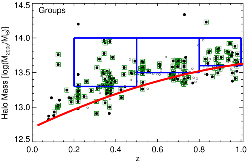
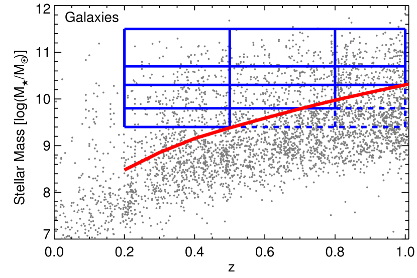
Figure 1.— Mass limits for groups (left) and galaxies (right) over the redshift range $0<z<1$. Symbols for groups denote their quality flags; green squares have xflag=1,2 and mask=poor=merger=0, black filled circles have xflag=1,2, and gray open circles are the rest. Red curves denote the mass sensitivity corresponding with the X-ray flux limit (left) and the stellar mass limits for a passive galaxy (right). Blue boxes show the mass and redshift bins used for analysis in § 7, with dashed boxes denoting stellar mass bins with significant incompleteness. Only every third galaxy is plotted for visual clarity.

3.2. Tests of Photometric Redshifts

We have described how the increase in photo-$z$ errors at faint magnitudes partially motivates our selection cut on galaxies brighter than F814W $=24.2$, with the implicit concern that poorer photo-$z$s degrade our ability to assign galaxies to groups. Here we test how photo-$z$ quality varies with other galaxy properties to ensure that our selection is not biased by systematic errors for certain galaxy populations.

In principle, photo-$z$ quality can depend on any property of an SED or the templates used in the fitting process. Redshifts of red galaxies with strong $4000$Å breaks have traditionally been easier to constrain than their bluer counterparts. Fainter galaxies have larger photometric uncertainties which propagate into their photo-$z$s. Galaxy mass and environment may play a role if, for example, the photo-$z$ templates are not representative of evolutionary histories unique to dense group regions. Morphology can also have a subtle effect since the inclination of disks alters the extinction along the line of sight (Yip et al., 2011).

Motivated by these possible sources of variation in photo-$z$ quality, we divide our sample into different populations and quantify the precision and accuracy of their redshift estimates. We also compare two estimates of photo-$z$ uncertainty, the $68\%$ width of the PDF ($\sigma_{\mathcal{P}}$), and the deviation between photometric and spectroscopic redshifts ($\sigma_{\Delta z/(1+\mbox{$z_{\rm s}$})}$).

In order to test the reliability of the redshift uncertainty for different galaxy populations, we slice the galaxy sample into bins based on their brightness, redshift, color, morphology, stellar mass, and environment. Here we use unextincted rest frame colors derived from the best-fitting templates using the difference between absolute magnitudes in near-ultraviolet (NUV) and R bands ($C\equiv M(NUV)-M(R)$) as described by Ilbert et al. (2010). In that paper, spectral classes were identified with the following cuts on $C$ from blue to red:

$$C<1.2$$ “high activity”

$$1.2<C<3.5$$ “intermediate activity”

$$C>3.5$$ “quiescent.”

These classes were found to correlate with visually classified morphologies as expected. For these tests, we use morphologies determined using the Zurich Estimator of Structural Types (ZEST; Scarlata et al., 2007) on the ACS images. The results are compiled in Table 1, in which we present the size and average magnitude of each population, along with the two measures of photo-$z$ uncertainty and the fraction of sources for which the photo-$z$ deviates significantly from the spectroscopic redshift.

The two independent measures of photo-$z$ uncertainty are in good agreement, suggesting that we can safely use PDF widths to quantify the precision of a given photo-$z$. Furthermore, we do not see strong trends in photo-$z$ quality with galaxy type or environment, and the outlier fraction is typically no larger than a few percent. In particular, the photometric depth in many bands and the treatment of emission lines in fitting SEDs by Ilbert et al. (2009) appears to balance the weakening $4000$Å break for bluer galaxies, so that photo-$z$ quality does not significantly depend on color. The lack of strong variations in photo-$z$ uncertainties, and the agreement between the two measures of photo-$z$ uncertainties across galaxy types and environments demonstrates the robustness of these redshifts for different populations. We have not included the photo-$z$s from Salvato et al. (2009) for AGN due to their rarity and the reasonable accuracy of the photo-$z$s of Ilbert et al. (2009) for these sources, but future work focusing on AGN may benefit from the improved redshift accuracy.

Table 1Photo-$z$ quality for galaxies with spectroscopic redshifts

Sample	$N_{obj}$	$\langle z\rangle$	$\langle\rm{F814W}\rangle$	med$(\mbox{$z_{\rm s}$}-\mbox{$z_{\rm p}$})$	$\sigma_{\Delta z}$	$\sigma_{\mathcal{P}}$	$\eta(\%)$
All	12370	0.52	21.3	0.003	0.012	0.013	1.1
Bright; low z	5768	0.31	20.7	0.001	0.009	0.011	1.0
Bright; high z	5613	0.71	21.6	0.006	0.015	0.014	1.0
Faint; low z	280	0.27	23.0	-0.002	0.014	0.016	3.9
Faint; high z	709	0.86	23.0	0.007	0.027	0.024	2.7
Bright; blue	6840	0.52	21.3	0.002	0.011	0.013	1.1
Bright; green	2548	0.44	21.0	0.006	0.014	0.013	1.2
Bright; red	1993	0.55	20.6	0.003	0.010	0.011	0.4
Faint; blue	731	0.70	23.1	0.000	0.021	0.021	3.8
Faint; green	259	0.64	23.2	0.011	0.028	0.027	2.7
Faint; red	67	0.92	23.1	0.013	0.031	0.020	7.5
Bright; early type	2450	0.53	20.4	0.004	0.011	0.011	0.8
Bright; late type	7248	0.49	21.3	0.003	0.012	0.013	0.7
Bright; irregular	1444	0.59	21.3	0.002	0.012	0.012	2.1
High stellar mass	4216	0.62	20.8	0.005	0.013	0.012	1.1
Low stellar mass	8154	0.47	21.5	0.002	0.012	0.013	1.2
Near groups	961	0.45	20.6	0.002	0.011	0.012	0.9
Outside groups	9691	0.54	21.4	0.003	0.012	0.013	1.2
Clean regions	10987	0.53	21.3	0.003	0.012	0.013	1.2
Masked regions	1439	0.51	21.2	0.003	0.013	0.012	2.5
MMGGscale	126	0.49	19.3	0.000	0.009	0.010	0.0
AGN	229	0.56	20.3	0.003	0.015	0.011	1.3

Note. — Brightness bins are divided at F814W=22.5 which is the limiting magnitude for zCOSMOS; redshift bins are split at $z=0.5$; color bins are $M(NUV)-M(R)<1.2$ (blue), $1.2<M(NUV)-M(R)<3.5$ (green), and $M(NUV)-M(R)>3.5$ (red); morphologies are categorized by ZEST; stellar masses are separated at $\log(M_{\star}/\mbox{$M_{\odot}$})=10.5$; group environments are classified as “near” within $R_{200\rm{c}}$ of an X-ray group center and where $|z_{s}-\mbox{$z_{\rm G}$}|/(1+\mbox{$z_{\rm G}$})<0.005$, and “outside” beyond $3\mbox{$R_{200\rm{c}}$}$ and where $|z_{s}-\mbox{$z_{\rm G}$}|/(1+\mbox{$z_{\rm G}$})>0.01$. Masked regions are areas in the optical images with bright foreground stars, satellite trails, or image defects. MMGG_scale are the most massive group galaxies within an NFW scale radius of the X-ray center (see § 4.3). AGN have been identified in Chandra X-ray data (Elvis et al., 2009).

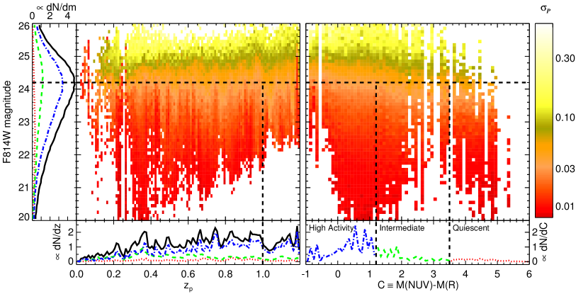
Figure 2.— Photo-$z$ uncertainties ($\sigma_{\mathcal{P}}$) as a function of magnitude and redshift (left), and color (right). Main panels show photo-$z$ uncertainty in bins colored according to the scale at right. Margin plots on the left side, bottom left, and bottom right show the magnitude, redshift, and color distributions, respectively. Curves are separated by color classification showing all galaxies considered (solid black), “high activity” galaxies (blue dot-dashed), “intermediate activity” galaxies (green dashed), and “quiescent” galaxies (red dotted). Dashed black lines show the galaxy magnitude and group redshift cuts at F814W=24.2 and $\mbox{$z_{\rm G}$}=1$ for the sample, as well as the divisions between color types. Ordinate axes on margin plots should be multiplied by $10^{4}$ (left side) and $10^{5}$ (bottom) for normalization. We do not see strong variations in photo-$z$ precision with redshift or color, but there is a significant magnitude-dependence.

While the photo-$z$ accuracy is good across the sample, the quality does decrease at fainter magnitudes. We account for this effect when selecting member galaxies by allowing larger tolerances in redshift space for fainter sources. There is also some degradation at higher redshift, but since our sample is not as heavily weighted toward high redshifts as it is toward faint magnitudes, we do not currently account for the redshift dependence of photo-$z$ accuracy when selecting group members. We note that Table 1 shows mean magnitudes and photo-$z$ errors for objects that also have spectroscopic redshifts; these errors are representative of the PDF uncertainties for the full galaxy sample in the bright bins, but in the faint bins the spectroscopic sample is brighter than the full population and photo-$z$ errors are smaller than average.

Figure 2 illustrates how the photo-$z$ PDF uncertainty varies with magnitude, redshift, and color for the full galaxy sample. The parameter space is divided into bins of $\Delta\mbox{$z_{\rm p}$}=0.01$, $\Delta\rm{F814W}=0.1$, and $\Delta C=0.1$. For bins containing at least 10 galaxies, the half-width of the median $68\%$ uncertainty on $\mathcal{P}(z)$ is computed and plotted according to the color scale shown. Additionally, we plot the redshift, magnitude, and color distributions of galaxies to characterize the catalog. Clearly the strongest trend in photo-$z$ precision is the decrease in quality at faint magnitudes, and there is only a weak dependence on redshift and galaxy color. Where the group member selection algorithm requires an estimate of redshift uncertainty, we consider only the magnitude dependence of the photo-$z$ uncertainties, ignoring the smaller variations due to color and redshift.

4. Group Membership Selection

4.1. Overview

This is not a paper about finding galaxy groups; instead our aim is to associate galaxies with groups that have already been identified as extended X-ray sources. Our basic strategy is to take the locations of groups from the X-ray catalog described in § 2.1 and Finoguenov et al. (2007, and in prep.) and assign galaxies to groups based on their positions and redshifts. Previous work on finding group and cluster members has often included assumptions about properties such as their red sequence content, luminosity function, and radial distribution. Because galaxy group populations have not been well-characterized in the mass and redshift range probed by this data set, we do not apply such filters to select members, with the hope that we can then measure these properties in an unbiased manner.

Effectively, we are selecting galaxies in a cylinder oriented along the line of sight around the X-ray position and redshift for each group. The radius chosen for this cylinder is the estimated $R_{200\rm{c}}$ of each group based on the total mass derived from the X-ray luminosity versus $M_{200\rm{c}}$ relation for the group sample as determined by weak lensing (Leauthaud et al., 2010). The depth of the cylinder in redshift space is allowed to vary for each candidate member galaxy according to the typical photo-$z$ uncertainty for its apparent magnitude (see Fig. 2).

Photometric redshift uncertainties are larger than the typical intrinsic span of a galaxy group in redshift space. A typical photo-$z$ error of $\sigma_{\mathcal{P}}=0.01$ in redshift-space corresponds to an uncertainty of roughly $40~{}\rm{Mpc}$ in distance along the line of sight, while a halo with $\log(\mbox{$M_{200\rm{c}}$}/M_{\odot})=13.5$ has a velocity dispersion of $\Delta\mbox{$z_{\rm G}$}\approx 0.001$ (Evrard et al., 2008) or a line of sight distance uncertainty of roughly $4~{}\rm{Mpc}$ at $z=0$. As a result, we must account for contamination of the member sample by galaxies at a similar redshift and position that do not belong to the group. One option is to subtract a mean background density from the number of galaxies found near the group. This statistical background subtraction can be extended to other quantities of interest, such as the total stellar mass in a group, by measuring those quantities averaged over regions away from the group and subtracting them from the values measured at the position of the group. One is left with the measured aggregate quantities for each group, but not a clear list of members and non-members. Another approach is to assign each galaxy a membership probability reflecting the likelihood that it belongs in a group, given some information about the relative number of field galaxies and group members. One can then determine properties of the group by selecting members above a given probability threshold, or by weighting members according to their probability of being a member.

We adopt this Bayesian approach to produce a group member catalog, which can in turn be used to measure a variety of properties about each group without requiring a new statistical background subtraction for each quantity. The selection algorithm thus assigns a probability of membership in a particular group to each galaxy given a number of observables: the projected separation of the group and galaxy in units of the group radius, the redshifts of the galaxy and group along with the typical photo-$z$ uncertainty for the magnitude of the galaxy, and an estimate of the number density of field galaxies relative to group members. Additionally, stellar masses are used to select a central galaxy from the membership list, refining the somewhat uncertain X-ray positions (see § 4.3).

4.2. Algorithm

In this section, we explain in detail how our selection algorithm works. We reiterate that our task is to identify galaxies that belong to groups rather than to find groups themselves. Our use of photo-$z$ PDFs to associate galaxies to known groups and clusters is similar to the method outlined by Brunner & Lubin (2000); we extend this method to incorporate varying photo-$z$ errors and a prior on the relative fractions of galaxies in groups and the field. The approach presented here was designed with COSMOS data in mind, but may be applicable to other multi-wavelength group and cluster studies, such as optical imaging surveys in fields with SZ or X-ray data. In § 5, we consider the quality of our resulting member catalog and how it could be modified by these different data sets. We attempt to keep the discussion here general while inserting details specific to the COSMOS data when necessary. To find the center of a group, we start with the X-ray centroid and then refine this position using the most massive member galaxy near the X-ray position, and finally we update the member list around the new central galaxy (more details on centering are presented in § 4.3 and Paper II.)

We first consider the field galaxies that can contaminate our selection. The background density of galaxies varies with position, redshift, and magnitude. We measure the number of galaxies in redshift bins ($\Delta z=0.05$) and magnitude bins (starting at F814W $<21.0$, then using a width of 0.8 mag, and ending at $23.4<\rm{F814W}<24.2$). This count excludes the volume within $3\mbox{$R_{200\rm{c}}$}{}$ and $z_{\rm{G}}\pm 5\sigma_{\mathcal{P}}(\bar{m})$ around all groups in the catalog regardless of flags, where $\bar{m}$ is the mean magnitude of galaxies in the bin. The final results are not strongly sensitive to the choice of volume removed around groups. Figure 3 shows this field density $n_{F}(\rm{F814W},z)=dN_{F}/dz/d\Omega$, which is similar to the quantity shown in the bottom left panel of Figure 2 but split into magnitude bins. Figure 3 also shows the field density as computed by summing the redshift probability distribution functions of galaxies for comparison to the approach of directly counting galaxies in photo-$z$ bins. Despite different sampling intervals ($\Delta z=0.01$ for the PDFs and 0.05 for bin counting), the methods show excellent agreement.

One can measure the background density locally around groups to account for correlated structure or globally across the field to increase the statistical sample with a larger volume, reducing noise. We have divided the COSMOS field into four separate quadrants to look for variations in $n_{F}$ with position and find that the values are in reasonable agreement across the field, with the density in individual quandrants deviating from the mean by typically no more than the Poisson errors. When smaller volumes are chosen to estimate the field density surrounding groups, the increased Poisson uncertainty swamps the constraint on locally correlated structure. We thus opt to use the entire area to estimate the mean density of background galaxies as a function of magnitude and redshift. We discuss further the choice of this method of estimating the field density in § 5.3.

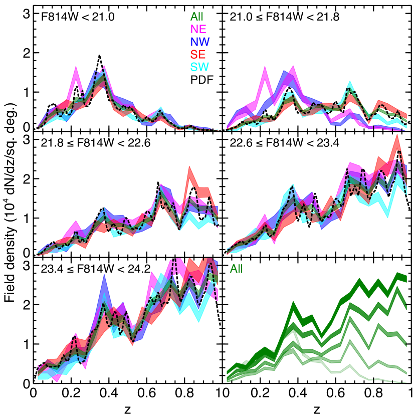
Figure 3.— Field density as a function of position, redshift, and magnitude. Different colored curves correspond to quadrants of the COSMOS field. The thickness of each curve corresponds to the Poisson uncertainty in each measurement. The dashed black line gives the stacked $\mathcal{P}(z)$ for all galaxies sampled at redshift intervals of 0.01, agreeing nicely with the measurement from counting galaxies in photo-$z$ intervals of 0.05. The variation between quadrants is not large, so we use the mean density across the whole field, shown by the green curve in each of panel and repeated in the bottom right panel for each magnitude bin.

We next consider candidate member galaxies, constructing a list of those objects in a cylinder with a projected distance from the group center less than $R_{200\rm{c}}$ and a redshift within $3\sigma_{\mathcal{P}}(m_{\rm max})$ of the group redshift $z_{\rm G}$, where $m_{\rm max}$ is the limiting magnitude F814W=24.2 and $\sigma_{\mathcal{P}}=0.035$. The number of member candidates can be compared with the field density in Figure 3 to estimate the fraction of galaxies that are group members.

For each candidate, we compare the photo-$z$ PDF to the expected redshift distributions of group members and field galaxies. We assume that each galaxy is either a group member (G) or part of the field (F), and assign a Bayesian membership probability using the relative sizes of the group and field populations as a prior to normalize the distributions. While the intial $3\sigma_{\mathcal{P}}$ cut uses the photo-$z$ value $z_{\rm p}$ to make a rough selection, here we use the full distribution $\mathcal{P}(z)$ for each galaxy to account for secondary peaks or other unusual features in the redshift PDF. The probability that a galaxy belongs to a group given $\mathcal{P}(z)$ can be written as

$$P(g\in G|\mbox{$\mathcal{P}(z)$})=\frac{P(\mbox{$\mathcal{P}(z)$}|g\in G)P(g\in G)}{P(\mbox{$\mathcal{P}(z)$})}.$$ (1)

The term $P(\mbox{$\mathcal{P}(z)$}|g\in G)$ is the likelihood of measuring the particular photo-$z$ PDF for a known group member. The prior $P(g\in G)=N_{G}/(N_{G}+N_{F})=1-P(g\in F)$ is based on the relative number of group and field galaxies in the cylinder, and

$$P(\mbox{$\mathcal{P}(z)$}) = P(\mbox{$\mathcal{P}(z)$}|g\in G)P(g\in G)+$$ (2)

$$P(\mbox{$\mathcal{P}(z)$}|g\in F)P(g\in F)$$

is the probability of measuring $\mathcal{P}(z)$ for any galaxy in the group or field. Each factor in Equation 1 has an implicit dependence on magnitude which we omit here and in following equations for notational simplicity, but we do account for magnitude-dependent variations in $\mathcal{P}(z)$ and in the field and group densities.

In order to compare the observed $\mathcal{P}(z)$ with that expected for a group or field galaxy, we must assume a distribution of redshifts for each population. Since the intrinsic velocity dispersion of groups is smaller than the uncertainty in $z_{\rm p}$  we model the true group redshift distribution as a $\delta$-function at $z_{\rm G}$, which is then convolved with a Gaussian of width $\sigma_{\mathcal{P}}(m)$ to account for photo-$z$ measurement uncertainty. We have tested the effects of modifying the true group redshift distribution to be broader than a $\delta$-function to account for intrinsic velocity dispersion but found this correction to be negligible. The redshift distribution of field galaxies is assumed to be uniform near $z_{\rm G}$ and remains unchanged after accounting for photo-$z$ measurement uncertainty. Each of these redshift distributions is convolved with the photo-$z$ PDF $\mathcal{P}(z)$ (note that $\int{\mathcal{P}(z)dz}=1$), giving

$$P(\mbox{$\mathcal{P}(z)$}|g\in G) = \int{\mathcal{P}(z)\mathcal{N}(\mbox{$z_{\rm G}$},\sigma_{\mathcal{P}})dz}$$ (3)

$$P(\mbox{$\mathcal{P}(z)$}|g\in F) = \int{\frac{\mathcal{P}(z)}{w(\sigma_{\mathcal{P}})}dz}$$ (4)

where $\mathcal{N}(\mbox{$z_{\rm G}$},\sigma_{\mathcal{P}})$ is a Gaussian centered on the group redshift with width equal to the typical $\mathcal{P}(z)$ uncertainty for the magnitude of the galaxy considered. The field density distribution is normalized so that the integral over the redshift range $\mbox{$z_{\rm G}$}\pm 3\sigma_{\mathcal{P}}$ is unity, so the width normalization parameter is $w(\sigma_{\mathcal{P}}(m))=6\sigma_{\mathcal{P}}(m)$. We have written these convolutions as indefinite integrals, but in reality they are discrete sums sampled at the redshift intervals $\Delta z=0.01$ and range $0\leq z\leq 6$ for which $\mathcal{P}(z)$ has been calculated. Because $\mathcal{P}(z)$ is sampled at intervals close to the typical photo-$z$ uncertainty, the distribution can effectively become a $\delta$-function, underestimating the true redshift error which has contributions from template uncertainties as well as photometric uncertainties. So we first convolve $\mathcal{P}(z)$ with a Gaussian of width d$z=0.01$ to account for these uncertainties and avoid sharply peaked PDFs.

To estimate the prior, $P(g\in G)$, we begin by counting the number of galaxies in the range $\mbox{$z_{\rm G}$}\pm 3\sigma_{\mathcal{P}}(m)$, measuring $N_{tot}=N_{G}+N_{F}$. The measurement of the field density shown in Figure 3 provides an independent estimate of $n_{F}$, which allows us to calculate an expected number of field galaxies in the cylinder, $\hat{N}_{F}=\int{n_{F}dzd\Omega}$. For each galaxy we linearly interpolate the curve in the relevant magnitude bin to the group redshift, and multiply $n_{F}$ by the volume searched around the group, $6\pi\mbox{$R_{200\rm{c}}$}^{2}\sigma_{\mathcal{P}}(m)$, to determine $\hat{N}_{F}$. This value is subtracted from the measured $N_{\rm tot}$ to determine the expected number of group galaxies in the cylinder, $\hat{N}_{G}$. We use the estimated values, $\hat{N}_{F}$ and $\hat{N}_{G}$, to determine $P(g\in G)$ and $P(g\in F)$, and Equation 1 assigns each galaxy a membership probability between zero and one. In cases where a group is not well-detected in a given magnitude bin $(N_{\rm tot}<\hat{N}_{F}$, i.e. $\hat{N}_{G}<0)$, galaxies in the bin are flagged and excluded from membership analysis. Tests in § 5 show that excluding these galaxies does not cause significant incompleteness in the member selection.

It is possible for the search cylinders of different groups to overlap, either because they reside in neighboring positions at the same redshift, or because of projections along the line of sight within the redshift uncertainties. In cases where a galaxy is a candidate member of multiple groups, each probability is recorded. A total of 4631 galaxies are assigned high probabilities of membership $(P_{\rm mem}\equiv P(g\in G|\mbox{$\mathcal{P}(z)$})>P(g\in F|\mbox{$\mathcal{P}(z)$})$, i.e. $P_{\rm mem}>0.5)$ in a group, and of these members only 163 or $3.5\%$ are also assigned to a second group. For most applications we can restrict our analysis to the highest group membership probability for each galaxy without any significant change in results, but recording each probability assignment will aid in the study of merging groups.

4.3. Group Centers

The robust identification of central galaxies is a challenging task, and relevant for a range of applications from satellite kinematics to stacked weak lensing to studying the most massive galaxies (e.g., Skibba et al., 2011). Miscentering is a significant source of systematic uncertainty in measuring the richness and weak lensing signal in optical groups (e.g., Johnston et al., 2007; Rozo et al., 2011; Rykoff et al., 2011). X-ray data and weak lensing offer additional information about the centers of mass of halos, which we use along with the galaxy content to guide our selection. We outline our approach to determining the optimal tracer of the center of mass here, and present our results in further detail in Paper II.

We use the X-ray position as an initial approximation of a group’s center, but for these faint detections the position can be uncertain by up to the wavelet detection scale of 32″($\sim 200~{}\rm{kpc}$ at $z=0.5$), so we consider other data to improve upon these constraints on the centers. Briefly, we have defined multiple candidate centers based on luminosity, stellar mass, and proximity to the X-ray center. By measuring the weak gravitational lensing signal stacked around each of these positions we can find the optimal center which maximizes the lensing signal at small radii. Our results indicate that this optimum center is the member galaxy (i.e., $P_{\rm mem}>0.5$) with the highest stellar mass within the scale radius plus the X-ray positional uncertainty of the X-ray center. We refer to this object as the MMGG_scale, for Most Massive Group Galaxy within the scale radius. We assign this galaxy to be the group center, and rerun the algorithm above to find members within $R_{200\rm{c}}$ of this galaxy for the final catalog.

Traditional visual selection of group and cluster centers includes looking for a bright, usually early type galaxy near the center of the X-ray or optical distribution, perhaps with an extended stellar envelope. Visual inspections of the Subaru, ACS, and XMM data support our objective selection, with broad agreement between the MMGG_scale and the objects one would traditionally identify as central galaxies. Visual selection becomes more ambiguous at high redshift and for groups lacking dominant galaxies, while our selection algorithm makes an objective choice. In a few percent of cases the MMGG_scale disagrees with a visually identified central galaxy due to photo-$z$ error or because of a significant offset from the X-ray position putting it outside the scale radius. We do not amend these cases, sacrificing a small degree of accuracy for a uniform and objective selection.

The selection of group centers used here is different than in Leauthaud et al. (2010), which employed a weighting based on stellar mass and distance to the X-ray position. Of the groups that have a confident central galaxy assignment from Leauthaud et al. (2010) and also satisfy the quality cuts for clean groups in § 3, $80\%$ are assigned the same central galaxy by the two methods, $9\%$ of the centrals identified by Leauthaud et al. (2010) are too distant from the X-ray center for our method to select, and $4\%$ are not identified as members with the current algorithm. In these cases of disagreement, the selection of Leauthaud et al. (2010) tends to favor more massive galaxies that are farther from the X-ray centroid than the selection used here, with average differences of 0.2 dex in stellar mass and $55~{}\rm{kpc}$ in distance to the X-ray centroid.

5. Purity and Completeness

Any selection of group members will have some fraction of false positives, interlopers selected as members that do not belong to a group, and false negatives, true member galaxies missed by the selection. To measure properties of member galaxies, we can weight each galaxy by its membership probability to account for these uncertainties. But we must test the reliability of those membership probabilities, and furthermore, for some applications we wish to define a set of galaxies exceeding a membership probability threshold with a reasonable degree of purity and completeness.

Purity and completeness are measures of overlap between the sample of selected members and the population of true members. We define the purity of the sample, $\mathsf{p}$, to be the fraction of selected members which are also true members. The completeness of the sample, $\mathsf{c}$, is the fraction of true members which are selected. Interlopers are objects which are selected but are not true members and missed galaxies are objects which are not selected but are true members. Formally,

$$\mathsf{p} = \frac{N_{\rm selected}-N_{\rm interlopers}}{N_{\rm selected}}$$ (5)

$$\mathsf{c} = \frac{N_{\rm true}-N_{\rm missed}}{N_{\rm true}}.$$ (6)

We can use the values of $\mathsf{p}$ and $\mathsf{c}$ to estimate $N_{\rm true}$ using $N_{\rm true}=N_{\rm selected}+N_{\rm missed}-N_{\rm interlopers}$ which can be rearranged into

$$\frac{N_{\rm true}}{N_{\rm selected}}=\mathsf{\frac{p}{c}}$$ (7)

using Equations 5 and 6. This correction factor, $\mathsf{p}/\mathsf{c}$, can be used to remove bias in the estimate of the intrinsic number of group members, $N_{\rm true}$, if we understand the purity and completeness of the selection algorithm.

To measure the purity and completeness of our member selection, we must have some way of telling which galaxies truly belong to groups. For our application, we use the subsample of objects with spectroscopic redshifts as well as mock catalogs to obtain knowledge of group membership that is independent of our photo-$z$ selection. The galaxies with spectroscopic redshifts allow us to test the photo-$z$ selection method on the same catalog, directly probing the effect of photo-$z$ uncertainties. But constraints on $\mathsf{p}$ and $\mathsf{c}$ are limited by the sparseness of spectroscopic coverage, and biases could be introduced since spectroscopic coverage is not representative of the full range of galaxies in the group sample. Furthermore, even spectroscopic selection of group members can have contamination and incompleteness (e.g., Gerke et al., 2005).

We perform further diagnostic tests using mock catalogs from N-body simulations described in § 5.2. Mock galaxies are prescribed to occupy halos according to a halo occupation distribution (HOD) model constrained by measurements of clustering, lensing, and stellar mass functions in COSMOS (Leauthaud et al., 2011a, b). After running the selection algorithm on a mock catalog, we can estimate its purity and completeness by comparing the results with the input list of group members. The mocks allow us to study greater volumes than the observed region, increasing statistical precision and providing estimates of the effects of sample variance for the volume probed. Mocks also give direct knowledge of galaxy group membership in real space without the redshift space distortions that mar spectroscopic selection, so we can study how the selection algorithm would perform on data sets with different errors in redshifts or positions. However, caution must be taken to ensure that the mock galaxies adequately represent the reality of correlated structure for all relevant properties, particularly in their distribution of positions, masses, and halo occupation.

In the following sections we describe in more detail our diagnostic tests on the selection algorithm using spectroscopic redshifts and mock catalogs. We begin by testing the tradeoff between purity and completeness for different membership probability thresholds, and proceed to study the principle sources of contamination and incompleteness in our selection.

5.1. Spectroscopic Tests

Here we consider the subset of galaxies with spectroscopic redshifts to measure the purity and completeness of the selection and study the effect of photo-$z$ errors. A “true” member in this case is defined to be a galaxy within $R_{200\rm{c}}$ of the X-ray center and with $c|\mbox{$z_{\rm s}$}-\mbox{$z_{\rm G}$}|<2\sigma_{\rm v}(\mbox{$M_{200\rm{c}}$},z)(1+\mbox{$z_{\rm G}$})$, where $c$ is the speed of light and $\sigma_{\rm v}(\mbox{$M_{200\rm{c}}$},z)$ is the velocity dispersion from the simulations of Evrard et al. (2008), assuming that the velocity bias between galaxies and dark matter is unity.

As we vary the membership probability threshold for photo-$z$ selection, we can see a tradeoff between purity and completeness shown in Figure 4 with black points from the spectroscopic test. Error bars show the standard deviation of 1000 bootstrap samples of the spectroscopic catalog. Restricting the member list to sources with membership probability $P_{\rm mem}>0.9$ gives a purity and completeness of $80\%$ and $19\%$ respectively. Lowering the membership threshold increases completeness while decreasing purity. In later sections, we use a threshold of $P_{\rm mem}>0.5$ as a compromise between these competing factors, which for the spectroscopic test produces a purity of $69\%$ and a completeness of $92\%$.

To further study the quality of the membership selection, we can measure trends in purity and completeness against other properties, seen in Figure 5. In this figure, we show how the selection performs for galaxies of different redshift, magnitude, stellar mass, group-centric distance, and group halo mass, by measuring the purity and completeness of objects assigned $P_{\rm mem}>0.5$. Figure 6 shows the same tests for color and morphology. The results are discussed in more detail in § 5.3, but we can see that the selection quality does not vary significantly with redshift or group mass, but does degrade in the outskirts of groups and for faint, low-mass galaxies, which also tend to have blue colors and late type morphologies. We have tested the influence of target selection effects on these results by restricting the spectroscopic sample to zCOSMOS galaxies which were uniformly selected at $i^{+}<22.5$. The purity and completeness measurements are consistent within the error bars of the full sample, but have slightly larger uncertainties due to the smaller sample size.

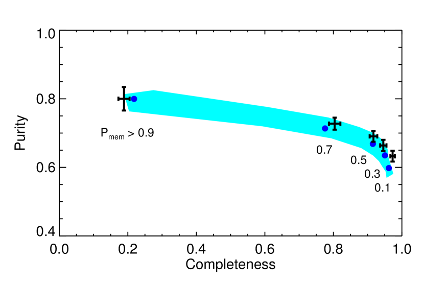
Figure 4.— Purity and completeness for different membership probability thresholds ($P_{\rm mem}>\{0.1,0.3,0.5,0.7,0.9\}$) as measured by the spectroscopic subsample (black crosses) and mock catalogs (blue circles, mean of ten lightcones). Error bars are the standard deviation from 1000 bootstrap samples of the spectroscopic catalog. The cyan shaded band is the region spanned by the ten mock lightcones.

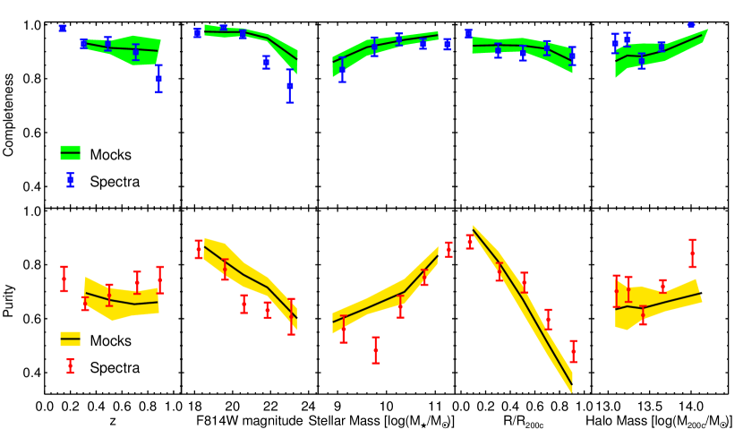
Figure 5.— Completeness (top row) and purity (bottom row) of the galaxy membership selection as measured by the spectroscopic subsample (points with error bars) and mock catalogs (shaded bands) for galaxies with $P_{\rm mem}>0.5$. Error bars are the standard deviation from 1000 bootstrap samples of the spectroscopic catalog, and shaded bands show the range spanned by the ten mock lightcones, while the solid black curve represents the mock mean. Bins were chosen to measure a roughly constant number of galaxies for each property tested while still representing the range of observed properties.

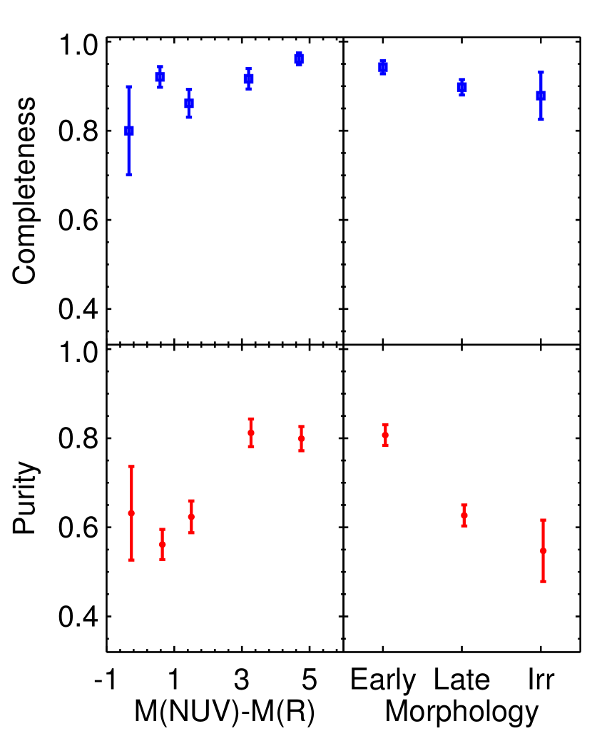
Figure 6.— Completeness (top row) and purity (bottom row) of the galaxy membership selection as measured by the spectroscopic subsample for galaxies with $P_{\rm mem}>0.5$. Error bars are the standard deviation from 1000 bootstrap samples of the spectroscopic catalog. Morphological classes are defined from ZEST (Scarlata et al., 2007); the early type category includes ellipticals (type=1) and bulge-dominated disks (type=2.0), the late type category includes the remaining type=2 sources, and irregulars have type=3.

5.2. Mock Catalogs

We use numerical simulations to construct a series of mock catalogs for a COSMOS-like survey to test the reliability of our member selection. Mocks are created from a single simulation (named “Consuelo”), part of the Las Damas suite (McBride et al., in prep.). Consuelo is a box of $420~{}h^{-1}~{}{\rm Mpc}$ on a side with $1400^{3}$ particles of mass $1.87\times 10^{9}~{}h^{-1}~{}{\rm M}_{\odot}$ and a softening length of $8~{}h^{-1}~{}{\rm kpc}$. This simulation can robustly resolve halos with masses above $\sim 10^{11}h^{-1}~{}{\rm M_{\odot}}$ which corresponds to central galaxy stellar masses of $\sim 10^{8.5}~{}h^{-1}~{}{\rm M_{\odot}}$, well-matched to our completeness limit of F814W=24.2 at $z=0.2$ (see Figure 1).

We extract ten light cones from the Consuelo simulation that have the same area as COSMOS and individually non-overlapping volumes. Halos within the simulation are identified with a friends-of-friends (FOF) halo finder (Davis et al., 1985) with a linking length of $b=0.2$. For typical halos in the mass range we consider, FOF masses and spherical overdensity masses (defined within a radius where the mean density is 200 times the background) typically agree within $\sim 10-20\%$ (Tinker et al., 2008); we thus only convert from background to critical overdensity to obtain $M_{200\rm{c}}$. Halos are populated with galaxies using the HOD model of Leauthaud et al. (2011a, b) that simultaneously fits the stellar mass functions, galaxy clustering, and galaxy-galaxy lensing signals of COSMOS. We adopt the $z\sim 0.6$ HOD model of Leauthaud et al. (2011b) with the following parameters from Table 5 of that paper: $\log(M_{1})=12.725$, $\log(M_{*,0})=11.038$, $\beta=0.466$, $\delta=0.61$, $\gamma=1.95$, $\sigma_{\log\rm M_{*}}=0.249$, $B_{\rm cut}=1.65$, $B_{\rm sat}=9.04$, $\beta_{\rm cut}=0.59$, $\beta_{\rm sat}=0.740$, $\alpha_{\rm sat}=1$. Details regarding the parameters in this HOD model can be found in Leauthaud et al. (2011a). As shown in Leauthaud et al. (2011b), there is a small amount of redshift evolution in this parameter set from $z\sim 0.2$ to $z\sim 1$. However, the redshift evolution should not have a large impact on our assessment of the completeness and purity of the group membership selection and so we neglect the redshift evolution of the HOD in this work.

Galaxies are assigned cosmological redshifts as well as mock spectroscopic redshifts which include the effect of peculiar velocities from the velocity dispersion within halos. Photometric redshifts are drawn from a Gaussian distribution centered around the spectroscopic redshift with width equal to the photo-$z$ uncertainty for that magnitude. A Gaussian $\mathcal{P}(z)$ is then centered at $z_{\rm p}$ with the same width, and sampled at the same redshift interval as the PDF for real galaxies. We do not include catastrophic photo-$z$ errors which are shown in Table 1 to be a small fraction of the sample.

The HOD model of Leauthaud et al. (2011a) assigns stellar masses to mock galaxies but does not assign magnitudes or colors. In order to apply a similar magnitude cut to the mock galaxies as used in the selection algorithm, we assign F814W magnitudes to mock galaxies. For each mock galaxy, we construct a galaxy sample from the COSMOS data that is matched in redshift and stellar mass in bins of $\Delta z=0.02$ and $\Delta\log(M_{\star}/M_{\odot})=0.2$. An F814W magnitude is assigned to each mock galaxy by randomly drawing a magnitude from the matched sample. We do not assign colors or morphologies to mock galaxies since the dependence of these properties on redshift and environment are not well-constrained. We will rely on our spectroscopic sample in order to determine the completeness and purity of the group membership selection as a function of color and morphology instead of using mock catalogs.

Mock halos are given the redshift of the central galaxy and X-ray luminosities according to the mean $L_{\rm X}-\mbox{$M_{200\rm{c}}$}$ relation of Leauthaud et al. (2010). To mimic the position uncertainties of the X-ray detections, xflag quality flags 1 or 2 are assigned randomly in proportion to their appearance in the COSMOS group catalog. The nominal group center is offset from the central galaxy with a Gaussian scatter of $32\arcsec$ for xflag = 2 halos which is reduced by the measured flux significance for xflag = 1 halos, and we assume a typical $5\sigma$ flux measurement. The impact of centroiding errors is investigated in § 5.4.

Next we run the membership algorithm described in § 4 on the mock galaxy and halo catalogs, associating galaxies with halos. We can perform the same purity and completeness tests as with the spectroscopic sample above, but this time we know the halo membership a priori. The results from these mock catalog tests are presented alongside those for the spectroscopic subsample as colored bands in Figures 4 and 5.

5.3. Sources of Error

Results from the tests on spectroscopic data and mock catalogs above can differ because the spectroscopic sample is weighted toward bright objects and because our knowledge of true membership in the spectroscopic data is limited by redshift-space distortions, while membership in the mock catalogs is known by design. The general agreement seen in Figures 4 and 5 between these tests of membership quality is encouraging, and it suggests that the biases are modest and that the mock catalogs accurately represent the properties of real galaxies that we wish to study. The normalization of the purity and completeness curves for the spectroscopic test has a degree of freedom in the velocity width used to determine whether a spectroscopic redshift is consistent with a group redshift. We used the criterion $c|\mbox{$z_{\rm s}$}-\mbox{$z_{\rm G}$}|<2\sigma_{\rm v}(M,z)(1+\mbox{$z_{\rm G}$})$ for spectroscopic membership; a broader velocity range for the spectroscopic test would result in a higher measured level of purity and lower completeness in the photo-$z$ selection, and the converse holds for a smaller velocity range, shifting the curves up or down. Though the absolute measure of purity and completeness in the spectroscopic tests holds some degree of arbitrariness, the relative trends shown in Figure 5 are in general agreement with the mocks, with some offsets likely due to sampling bias and redshift-space distortions. We study the effects of redshift-space distortions on member selection in the limit of a completely spectroscopic survey in § 5.4.

Information from the spectroscopic tests has the advantage that it can probe member selection effects due to properties that cannot easily be modeled (e.g., galaxy color and morphology), and these tests directly measure the effects of photo-$z$ errors on our selection of galaxies in the same set of groups. We see in Figure 6 that the trends of selection quality with color and morphology parallel the trends with magnitude and stellar mass from Figure 5. We have shown in § 3.2 that photo-$z$ quality is not strongly affected by color or morphology, and no other inputs to our selection algorithm explicitly depend on these properties. We infer that the lower completeness and purity seen for faint, low mass, blue, and late type galaxies is driven by two effects; fainter galaxies have larger photo-$z$ uncertainties, and galaxies in this population tend to live outside of dense groups so that they are more likely to be contaminants when selected.

Because only a fraction of objects have spectroscopic redshifts, the uncertainties can be large. Tests with mock catalogs alleviate this issue and provide an estimate of the sample variance in our selection due to the finite size of the COSMOS region. An additional advantage of the mocks is that the central galaxy of each halo is known, so we can test the success rate for identifying these objects. We find that $77\%$ of central galaxies are correctly identified as the MMGG_scale galaxies in the corresponding halos, $12\%$ are misidentified as satellites because the central galaxy is not the most massive member near the centroid, $5\%$ are misidentified as satellites because the assigned centroid error puts the galaxy outside of the search region, and only $5\%$ are assigned to neighboring groups or the field due to photo-$z$ errors. While the HOD used to create the mocks allows for satellite galaxies to be more massive than centrals due to scatter in the relation between stellar mass and halo mass, the fraction of groups where this occurs is sensitive to the parametrization of the HOD model and is not well-constrained. The problem of identifying group centers will be discussed in more detail in Paper II.

For the full sample of mock galaxies with $P_{\rm mem}>0.5$, we find a mean purity of $67\%$ and completeness of $92\%$. Looking at Figure 5, it is clear that the dominant source of impurity comes from galaxies in projection near the outskirts of groups. We can attribute this contamination to the fact that the density of true members falls steeply as a function of distance from group centers while our membership algorithm selects galaxies uniformly out to $R_{200\rm{c}}$. Faint galaxies are another source of impurity since their photo-$z$ errors are larger than average. Galaxies with lower masses and bluer colors are more common in the field than in dense environments (see § 7), so a higher contamination fraction from these populations is to be expected. There is also a slight dependence on halo mass, since the density contrast between the field and groups is smaller for low mass halos, lowering the assigned membership probabilities of candidate members and reducing the completeness of the selection. These factors motivate the use of matched filters in finding groups and clusters when the properties of their galaxy populations are well-characterized; we have not employed such filters to avoid biasing our sample and because galaxy properties in this range of halo masses and redshifts are not thoroughly constrained.

The covariance between these galaxy properties makes it challenging to isolate their influence on the contamination fraction. For example, the correlation between the stellar mass and brightness of a galaxy means that the corresponding panels of Figure 5 are related and not independent probes of contamination sources. The simplest way to increase the purity of the group sample is to consider only galaxies at smaller distances from the group center than the cut of $R_{200\rm{c}}$ used here. Restricting the mock sample to $R<0.5\mbox{$R_{200\rm{c}}$}$ results in a mean purity and completeness of $84\%$ and $92\%$, respectively.

An alternative way to address the contamination and incompleteness of the selection would be to apply correction factors to the member selection as a function of these properties, as in Equation 7. This would amount to introducing strong priors to the membership algorithm based on our HOD model, limiting the independence of the sample. In testing this approach however, we have noticed that the correction factor as a function of group-centric radius is not significantly tied to other properties such as magnitude, stellar mass, or color, indicating that the contamination is due more to geometry than distinct populations of galaxies. This suggests that we can reliably study the relative radial trends of these properties, though the absolute radial trends are subject to uncertainties in the correction factor.

We can compare the member selection used here with that of Giodini et al. (2009), who used a statistical background subtraction on the same body of data to determine galaxy membership and estimate the total stellar mass in groups. Because the statistical background approach does not individually assign galaxies to groups, we cannot directly compute the purity and completeness of the selection, but we can compare the total stellar mass estimates from the two selection methods to the mock values. Giodini et al. (2009) selected candidate members within a projected radius $R_{500\rm{c}}$ of X-ray centroids and $0.02\times(1+z)$ of the group redshift, and estimated a mean foreground/background contribution in 20 non-overlapping field regions of the same size and redshift.

We run both member selection methods on the mocks, applying to each method the same corrections described by Giodini et al. (2009) to deproject the cylindrical search volume into a sphere of radius $R_{500\rm{c}}$ and to account for stellar mass contributions below our sensitivity limit, adapted to the stellar mass function and limits of our mocks. The mean stellar mass content in groups recovered using their method is $3\%$ lower ($3\%$ higher) than the input mock value in the redshift range $0.2<z<0.5$ $(0.5<z<1.0)$. With the same corrections, our selection method estimates the mean stellar mass to be $3\%$ higher ($9\%$ higher) than the mock values over the same redshift intervals. The typical scatter of $35\%$ between the recovered values and the input values for a given group is much larger than the offsets for both methods, but with these tests on mock catalogs we could remove the small biases in future measurements. The mean stellar masses inferred by the two methods happen to be quite similar because they are typically dominated by massive galaxies for which membership assignment is relatively straightforward. However, we note that the full membership selected can be quite different because our approach optimizes group centers using the weak lensing signal and handles magnitude-dependent photometric redshift uncertainties, whereas Giodini et al. (2009) use the X-ray centers and a fixed redshift window.

We can also test different methods of estimating the field density to see how it influences our member selection. Our selection algorithm estimates $\hat{N}_{F}$ from the mean density across the whole field, but smaller regions could instead be used to estimate the local density around individual groups. While the local density estimate has the advantage that it traces correlated structure around groups, it does suffer from greater shot noise than the density estimated over a larger volume. We have tested our approach by using annuli centered on each group with inner and outer radii of $2\mbox{$R_{200\rm{c}}$}$ and $5\mbox{$R_{200\rm{c}}$}$, while keeping the rest of the selection algorithm the same. With this approach, the typical field density is higher due to clustering around groups and the resulting membership probability is slightly lower (increasing the field density by a factor of 2 typically lowers the membership probability by only $\sim 20\%$), but the purity and completeness of the sample are essentially unchanged, and the fraction of members crossing a threshold of $P_{\rm mem}>0.5$ between samples is less than $10\%$. We obtain similar results when substituting the background estimation method used by Giodini et al. (2009) for our field density prior, so the selection algorithm is not strongly sensitive to the approach used for background estimation.

5.4. Applicability to Other Surveys

In view of other surveys which will search for groups and clusters in multi-wavelength data, and to better characterize the advantages or shortcomings of the COSMOS data used in this analysis, we test our selection algorithm on mock catalogs with different levels of uncertainty in redshift and centroid measurements. We consider five hypothetical data sets: a full spectroscopic survey where all galaxies have the typical redshift uncertainty in zCOSMOS of $\sigma_{z}=3.7\times 10^{-4}$, a low-resolution spectroscopic survey like PRIMUS (Coil et al., 2010) with redshift uncertainties of $\sigma_{z}=0.005$, a photometric survey with fewer bands and larger photo-$z$ errors like SDSS (Csabai et al., 2003) or DES (Banerji et al., 2008) with $\sigma_{z}=0.05$, a deeper X-ray survey with more precise centroids of $3\arcsec$, and a lower resolution X-ray or SZ survey with centroid uncertainties of $1\arcmin$. In the first three mock surveys we vary only the redshift uncertainty and apply the same centering uncertainty as the fiducial COSMOS mocks described in § 5.2 assuming similar X-ray detections. In the final two mock surveys we use the magnitude-dependent redshift uncertainties of the COSMOS mocks and assign centroiding uncertainties, $\sigma_{\rm X}$, in each dimension on the sky. We offset the nominal centroid from the central galaxy in each dimension by a random value drawn from a Gaussian of width $\sigma_{\rm X}$. In all cases we keep the same group and galaxy detection limits as in the COSMOS data.

Figures 7 and 8 show the purity and completeness obtained when applying our member selection algorithm to these mock surveys, in a manner similar to Figure 5. We reiterate that these statistics describe the accuracy of the assignment of galaxies to groups, and not the detection of groups themselves. The figure illustrates that purity and completeness improve as redshift and centroid uncertainties decline. A number of other points can be made about these results:

• Deeper and more complete spectroscopic coverage would improve our member selection, increasing the purity of the sample from $\sim 70\%$ with photo-$z$s to $\sim 85\%$. Improvements for completeness would mainly be gained from faint galaxies near our magnitude limit.

• Among spectroscopic redshifts, high precision is not critical. The completeness of the $\sigma_{z}=3.7\times 10^{-4}$ and $0.005$ samples are nearly identical, and the higher precision spectra provide only a modest improvement in sample purity over the low-resolution spectra, from $\sim 80\%$ to $\sim 85\%$. Once the redshift measurement uncertainty becomes comparable to the magnitude of intrinsic redshift distortions due to peculiar velocities in groups, additional spectral resolution does not greatly improve our ability to identify members. PRIMUS data in the COSMOS field will improve upon the existing sampling of zCOSMOS, but we note that the completeness limit for that survey is $i=22.5$ with sparse sampling to $i=23.5$, still shallower than our photo-$z$ depth of F814W=24.2.

• The precise photometric redshifts available in the COSMOS field are critical for identifying members using our approach. Redshifts that are less accurate or precise show significantly reduced purity and completeness.

• The precision of X-ray centroids for COSMOS groups is quite sufficient for member selection. Improving the positional uncertainty by roughly a factor of eight from the mean COSMOS value results in only a few percent improvement in completeness and a negligible gain in purity. Conversely, less precise centers (such as those available from SZ measurements) produce a sample with lower purity in the central region ($\sim 85\%$ instead of $\sim 95\%$) and significantly lower completeness ($\sim 75\%$ instead of $\sim 90\%$). Though the existing COSMOS centroids are adequate for assigning member galaxies to groups, we note that several aspects of groups could still be studied with deeper X-ray or SZ data including physical offsets between central galaxies and hot gas, and the relationships between temperature or entropy with other group properties.

• Note that we do not optimize our selection algorithm for these hypothetical data sets. Combining catalogs built from different observables (e.g., Cohn & White, 2009), and other techniques such as iterative centering or matched filters could improve results.

We can compare the results of our mock spectroscopic selection to other methods in the literature. We must note that our definitions of purity and completeness refer to the success rates for assigning members to known groups, while previous spectroscopic group-finding efforts have typically quantified the purity and completeness of the identified group catalog in addition to the galaxy membership assignment. In our mock tests, we have implicitly assumed that the identification of groups is pure and complete. It is also difficult to make direct comparisons across surveys because of differences in data sets, limiting depths, and mock catalogs. However, looking briefly at the quoted purity and completeness of spectroscopic group catalogs, we can assess our algorithm and see the advantage to assigning group membership when the existence of a group is already know (e.g., from an X-ray detection).

Using a tesselation method to find galaxy groups in DEEP2 with a limiting galaxy magnitude of R${}_{\rm AB}=24.1$, Gerke et al. (2005) attained a mean interloper fraction (analogous to our impurity, $1-\mathsf{p}$) of $f_{I}=0.458\pm 0.004$ and a mean galaxy success rate (analogous to our completeness) of $S_{\rm gal}=0.786\pm 0.006$ in their mock tests. They reported a one-way group identification purity of $P_{1}=0.545\pm 0.005$ and completeness of $C_{1}=0.782\pm 0.006$. Knobel et al. (2009) found that a friends-of-friends approach performed better than the tesselation method for identifying groups in zCOSMOS to a limiting magnitude of I${}_{\rm AB}=22.5$, and reported values of $f_{I}=0.29$, $S_{\rm gal}=0.84$, $P_{1}=0.66$, and $C_{1}=0.81$ from their mocks. These values are for groups with $N_{\rm mem}\geq 2$, and while Gerke et al. (2005) showed values for group purity and completeness that were roughly constant with group velocity dispersion, Knobel et al. (2009) showed that each of these statistics improved when restricting the sample to higher richness groups, flattening out for groups with $N_{\rm mem}\gtrsim 5$. Disentangling the effects of group identification from galaxy membership assignment is difficult, but since the reported $S_{\rm gal}/C_{1}$ and $(1-f_{I})/P_{1}$ are both approximately unity, it appears that the main challenge in assigning galaxy membership with these algorithms is in identifying real groups. This fact illustrates the advantage of combining group-finding methods to ensure a reliable sample of groups before assigning members.

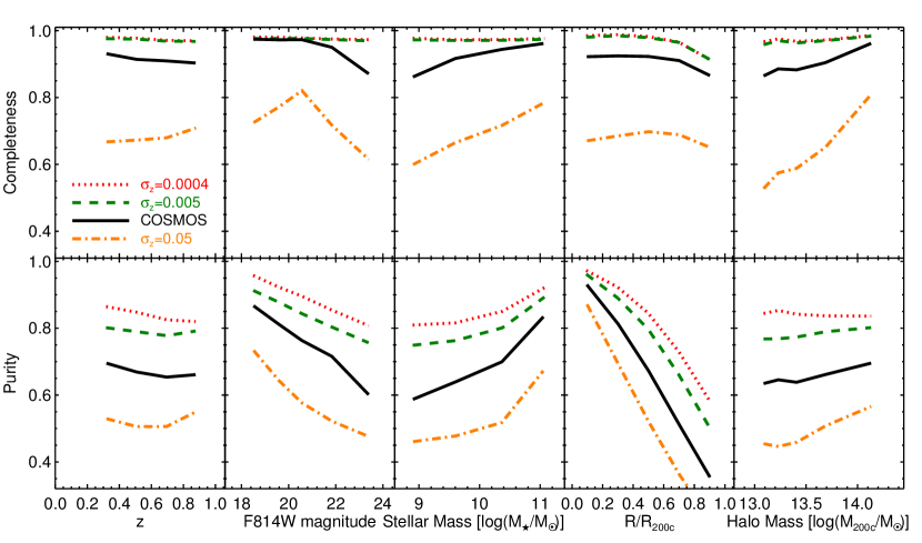
Figure 7.— Completeness (top row) and purity (bottom row) of the galaxy membership selection for hypothetical surveys with different redshift uncertainties according to the legend. Each curve represents the mean of ten mock lightcones. The fiducial survey is the same as that plotted in Figure 5 for COSMOS. Note that the completeness curves for $\sigma_{z}=0.0004$ and $0.005$ lie atop one another.

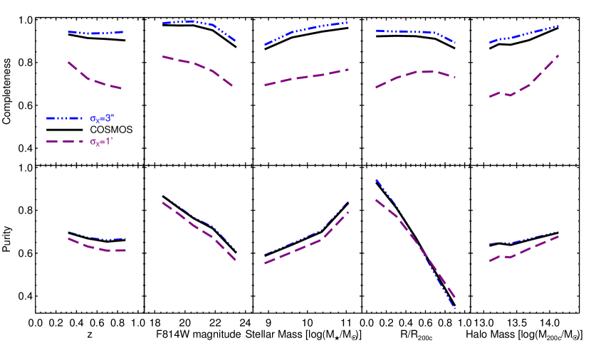
Figure 8.— Completeness (top row) and purity (bottom row) of the galaxy membership selection for hypothetical surveys with different centroid uncertainties according to the legend. As in Figure 7, each curve represents the mean of ten mock lightcones, and the fiducial survey is the same as that plotted in Figure 5 for COSMOS.

6. Member Catalog

In the spirit of public releases of COSMOS data, we make our membership assignments available as machine-readable files through the NASA/IPAC Infrared Science Archive (IRSA). These data include galaxy positions, redshifts, stellar masses, colors, and membership probabilities, along with group identifications. For each group we provide the X-ray position, flux, and luminosity, along with the redshift, halo mass, quality flags, and the position and stellar mass of the central galaxy MMGG_scale. For reference, the basic parameters describing the catalog are compiled in Table 2. For analyses requiring a clean selection of galaxy groups, we restrict the sample to groups with xflag $=1$ or 2 and the mask, poor, and merger flags blank to ensure that groups and members have been reliably identified; in the group catalog we define a new property, flag_include, to encode this combination of selection cuts. When a pure and complete sample of members is needed, we select galaxies with $P_{\rm mem}>0.5$ in the inner regions of groups, $R<0.5\mbox{$R_{200\rm{c}}$}$, with stellar masses above our sample limit shown in Figure 1.

Table 2Basic catalog properties

Property	Value
Field coordinates (J2000)	RA=(149$\fdg$4, 150$\fdg$8), Dec=(1$\fdg$57, 2$\fdg$90)
Group redshift	$0<\mbox{$z_{\rm G}$}\ <1$
Galaxy magnitude	F814W $<24.2$
Halo mass	$12.8<\log(\mbox{$M_{200\rm{c}}$}/M_{\odot})<14.3$
X-ray luminosity	$41.3<\log(L_{\rm X}/\mbox{erg s${}^{-1}$})<44.1$
Ngroups	$211$
Ngroups (xflag $=1,2$)	$165$
Ngroups (clean groups)	$129$
N${}_{\rm mem}(P_{\rm mem}>0.5)$	$4631$
N${}_{\rm mem}(P_{\rm mem}>0.5$, clean groups)	$3406$
N${}_{\rm mem}(P_{\rm mem}>0.5,R<0.5\mbox{$R_{200\rm{c}}$},\log(M_{\star}/M_{\odot})>10.3)$	$868$
N${}_{\rm mem}(P_{\rm mem}>0.5,R<0.5\mbox{$R_{200\rm{c}}$},\log(M_{\star}/M_{\odot})>10.3$, clean groups)	$657$

In addition to the catalog described above using photometric redshifts, we have also produced a catalog replacing photo-$z$s with spectroscopic redshifts when available. We use the same selection algorithm and replace $\mathcal{P}(z)$ from the photo-$z$ with a Gaussian of width equal to the typical uncertainty in zCOSMOS, $\sigma_{z}=3.7\times 10^{-4}$, and sample each distribution at intervals of $10^{-5}$ in redshift. This catalog has better purity and completeness than the photo-$z$ catalog because of the improved redshift accuracy, but the selection is less homogeneous because spectroscopic sampling is not representative or complete.

7. Analysis and Discussion

With the catalog of group members identified and the purity and completeness of the sample characterized, we provide a first look at the properties of galaxies in these groups. Here we present an analysis of the colors of group members relative to the field. Future papers will study member properties in more detail, including galaxy morphologies, star formation rates, and AGN activity with respect to group properties like redshift, halo mass, and group-centric distance.

Figure 9 shows the unextincted rest-frame NUV-R colors from Ilbert et al. (2010) for group members. We use the clean sample of groups, selecting members with $P_{\rm mem}>0.5$ within $R_{200\rm{c}}$ of the group center. The apparent banding in colors is due to the finite number of templates used. We call galaxies identified as the MMGG_scale “centrals” with the other members as “satellites.” We see a bimodal distribution in color space for both central and satellite galaxies, though redder colors are more common than blue for both types of members. In the margin plots, we show the distributions of colors and stellar masses for centrals and satellites, as well as field galaxies not assigned to any X-ray detected group ($P_{\rm mem}=0$). The field sample has been selected to match the redshift distribution of group members in bins of $dz=0.1$. Although the color distribution of field galaxies is also bimodal, it is clear that bluer galaxies are more common in the field than in groups, a well-known result in clusters and dense environments over a range of mass scales and redshifts (e.g., Gerke et al., 2007).

We also see that there exist a number of blue centrals, which are of interest because they suggest that star formation can persist or be reactivated in the centers of dense groups, or that AGN exist there. The set of red points in Figure 9 omits ambiguous cases where there is a more massive galaxy in the outskirts of a group or where the MMGG_scale differs between the photo-$z$-only catalog and the one supplemented with available spectroscopic redshifts; $79\%$ of groups satisfying the quality cuts of § 6 have an unambiguous central according to these criteria. While the majority of this sample of centrals are red (77 out of 102), there are 5 centrals with blue colors indicative of active star formation or AGN, and 20 centrals with colors indicating intermediate activity. This population warrants further study to verify that they are accurate centers and to determine what environmental factors could contribute to the star formation or AGN activity.

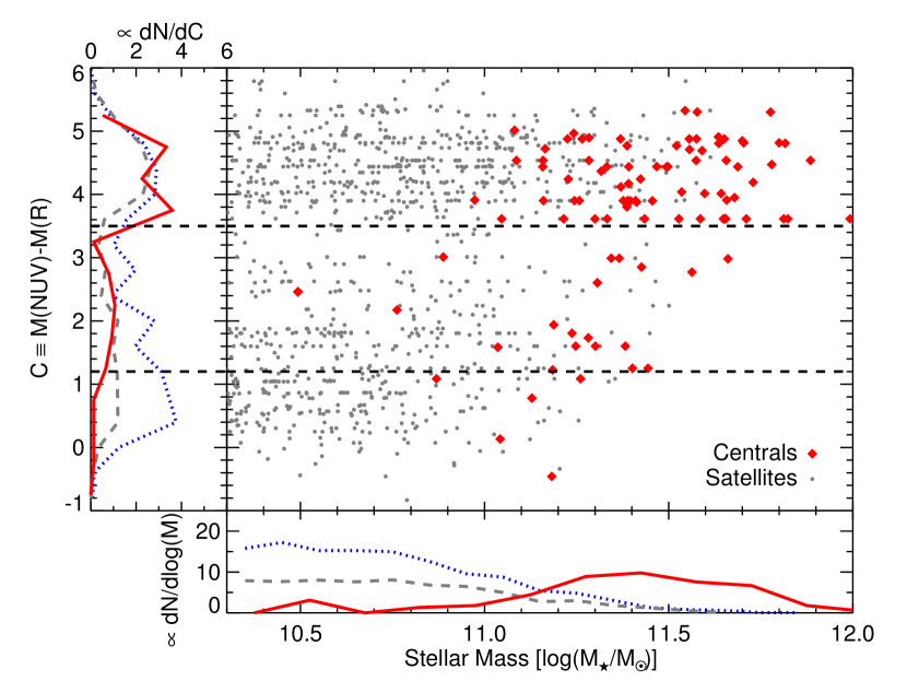
Figure 9.— Stellar masses and unextincted rest-frame template colors for central galaxies (red diamonds) and satellites (gray dots). We plot only the unambigous centrals, i.e.those designated as the MMGG_scale in groups which do not have a more massive galaxy in the outskirts or a discrepancy between identification with spectroscopic and photometric redshifts. Horizontal dashed black lines show the galaxy spectral classes of Ilbert et al. (2010). Margin plots show the distribution of colors and stellar masses for centrals (red solid), satellites (gray dashed), and a redshift-matched sample of field galaxies (blue dotted), rescaled for comparison. Axis labels should be multiplied by 15 (centrals), 150 (satellites), and 500 (red-shift matched field sample) to obtain the normalized distributions. The lower end of the stellar mass range plotted corresponds to our completeness limit at $z=1$.

7.1. Environmental Dependence from $z=0.2$ to $1$

The higher fraction of blue galaxies in the field compared to groups shown in Figure 9 indicates that star formation is less common in dense environments. As discussed in the introduction, much work has been carried out to determine whether this well-known effect is due to a physical process acting on galaxies in dense enviroments to suppress their star formation rates, or due to the intrinsic properties of galaxies that exist in these regions.

To distinguish between the possibilities of environmental influence and innate differences, we compare galaxy colors in group and field environments within fixed stellar mass bins. We measure the fraction of galaxies of the quiescent type defined by Ilbert et al. (2010), i.e. those with $M(NUV)-M(R)>3.5$. These are unextincted rest-frame colors from the spectral template that best fits each galaxy’s SED, allowing us to study intrinsic colors that are related to specific star formation rates without the obscuring effects of dust. The correction is important because galaxies in low density environments have a higher dust content, even among massive galaxies (Kauffmann et al., 2004).

The fraction of red galaxies in fixed stellar mass bins is plotted for three redshift ranges in Figure 10. For group members, we consider only galaxies with membership probability $P_{\rm mem}>0.5$ within a projected distance of $0.5\mbox{$R_{200\rm{c}}$}$ of the center of groups in the mass completeness-limited bins of Figure 1. The radial cut on the group sample is to avoid contamination in the outskirts discussed in § 5.3. The plot includes both centrals and satellites; excluding centrals leaves the results essentially unchanged because the sample is dominated by satellites even in the highest stellar mass bin plotted. The fraction of red galaxies in this population is plotted against the mean stellar mass for each bin. We also plot the red fraction in individual groups for galaxies in the same stellar mass bins to show the variation between groups. At all redshifts, higher mass galaxies tend to have higher red fractions than lower mass galaxies. In addition to this stellar mass dependence, we see a clear separation between the group and field populations at all redshifts for the stellar masses probed. The field sample plotted matches the the redshift bins used for group members; matching the redshift distribution on finer scales results in quenched fractions that are at most a few percent different from those plotted.

We also see evidence for an increase in the red fraction with decreasing redshift among low mass group galaxies. Redshift trends are somewhat difficult to interpret because the range of group masses used is different in each redshift bin (see Figure 1) and the color cut does not account for evolution, so we leave a detailed analysis for future work. Because our galaxy sample is magnitude-limited, the low mass bins at high redshift are incomplete and plotted as open symbols. We make no corrections for incompleteness here, which likely leaves the sample in these bins biased toward the detection of blue galaxies that tend to have lower mass-to-light ratios than red galaxies, so we consider the red fractions in incomplete bins to be lower limits.

Figure 10.— Fraction of quenched galaxies as a function of stellar mass in different redshift bins (separate panels). Triangles show the quenched fraction of members with $P_{\rm mem}>0.5$ and projected group-centric distance within $0.5$$R_{200\rm{c}}$ of groups in the mass bins from Figure 1. Squares show the quenched fraction of field galaxies with $P_{\rm mem}=0$. Open symbols show bins with stellar mass incompleteness; the arrows above these symbols indicate that they are likely to be biased lower than the true values. Vertical error bars show the standard deviation of 1000 bootstrap samples and horizontal bars represent the stellar mass bin widths. Gray circles show the quenched fraction in a given stellar mass bin for individual groups, with size proportional to the number of members in the bin. Note that the range of halo masses for group members varies between redshift bins.

We detect a clear dependence of galaxy color on environment, even at fixed stellar mass and high redshift. Figure 10 uses the member catalog determined with photometric redshifts only, but including the available spectroscopic redshifts does not affect the results. Our results are similarly insensitive to the choice of a probability threshold for membership; changing the cut on $P_{\rm mem}>0.5$ to 0.3 or 0.7 or weighting objects by $P_{\rm mem}$ instead of choosing a threshold moves the red fractions by no more than a few percent in any bin. Using the color cuts described in Bundy et al. (2010) to separate passive galaxies in COSMOS from dusty star-forming galaxies also gives qualitatively similar results. Though the absolute fraction of red galaxies measured depends on the specific cuts used, the relative trends with stellar mass and environment are similar; galaxy groups have a larger proportion of red galaxies than the field, and groups dominated by blue galaxies are rare, though some appear to exist.

We note that while our results confirm a significant relationship between color and environment out to the redshift limit of our sample, the cause of this relationship remains unknown. More detailed analysis distinguishing between physical processes happening before and after galaxies join groups is necessary to determine the role that groups play in this process.

We now compare Figure 10 to results from the literature. Our findings are consistent with results at low-redshift that show a decrease in star formation at high stellar masses, as well as a clear connection between star-formation and environment even after accounting for stellar mass differences (e.g., Kauffmann et al., 2004; Baldry et al., 2006). At $z\sim 0.4$, McGee et al. (2011) report an environmental trend in the GEEC survey that is smaller than a comparable low-redshift sample, but still significant. However, Poggianti et al. (2008) do not detect a significant separation in the fraction of star-forming galaxies in cluster and field environments at $z=0.4-0.8$ after matching stellar mass distributions.

At the highest redshift range covered by our group sample, our findings are consistent with those of Cooper et al. (2010) and Peng et al. (2010) who detect a significant color-density relation in a similar stellar mass range covered by DEEP2 and zCOSMOS, respectively. These results appear to be at odds with some claims from VVDS and zCOSMOS analyses that such a relation could be attributed solely to the existence of more massive galaxies in dense environments (e.g., Scodeggio et al., 2009; Cucciati et al., 2010; Iovino et al., 2010). Each of these studies consider the environmental effect on color at fixed stellar mass, as we have done here. Cooper et al. (2010) emphasize that systematics in the selection of dense environments tend to wash out the measured signal of environmental dependence, so that if such correlations are seen they are likely to be real. They also suggest that the non-detection of environmental trends in other surveys is likely due to lower spectroscopic sampling rates and reliance on less confident redshifts which comprise a significant fraction of the sample at high redshift. The photometric redshifts used in the present work are certainly less precise than spectroscopic redshifts, but have a much higher sampling density.

An important distinction with this study is that we are using a unique sample of groups; X-ray detections ensure a robust sample of structures that are virialized, a trait which may not be true of optically-selected groups. The X-ray groups are also more massive than the typical spectroscopically-selected groups, and may have formed earlier giving them a longer time to suppress star formation in member galaxies. Other studies of this sample of X-ray groups also detect a significant environmental effect on galaxy colors (Giodini et al., in prep.; Tanaka et al., in prep.). Finoguenov et al. (2010) have shown that the number density of this X-ray group sample is in reasonable agreement with that expected for halos of corresponding masses within our cosmological model. The sample is therefore unlikely to be an extreme population of groups, though we cannot rule out subtle differences between X-ray-selected groups and the full population of groups in this mass range.

Because of differences in analysis methods, it is difficult to determine whether the qualitatively distinct findings in these environmental studies are also quantitatively inconsistent, or whether different results are simply due to measuring different quantities. We now consider aspects of the analysis methods and definitions of environments that may contribute to the differing results, focusing our attention to field studies at $z\sim 1$ where the results appear most discrepant. For instance, we have shown in Figure 8 that centroiding errors can influence the purity and completeness of a group sample, and our lensing tests (see Paper II) ensure a reliable determination of the center of mass. Additionally, we use only galaxies and groups in mass-complete bins, avoiding the need for volumetric corrections made in some of the previous analyses.

Our group-based definition of dense environments is most similar to that of Iovino et al. (2010), who studied optically selected groups which are less massive on average than the X-ray groups studied here. We leave a detailed comparison between optically and X-ray selected groups in COSMOS to a future paper (Finoguenov et. al, in prep.), but Figure 22 of Kovač et al. (2010b) shows that these X-ray selected groups tend to be in more dense regions on average than the optically selected ones. The richest optical groups (with 4 or more members) show a good correspondence with X-ray groups in the density field and are more likely to have similar halo masses. Figure 12 of Iovino et al. (2010) shows that the colors of stellar mass-selected samples do not significantly depend on group richness (except perhaps at low stellar mass and redshift), so the difference in halo masses between X-ray and optical groups is not obviously the cause of discrepancy between our results and those of Iovino et al. (2010). Knobel et al. (2009) tested the purity of the optical group sample with mock catalogs and found a contamination fraction of roughly $25\%$, improving to about $15\%$ for richer groups. These values are similar to our estimate of $16\%$ contamination within $0.5\mbox{$R_{200\rm{c}}$}$ for the sample used in our analysis, so the correct identification of group members is not a clear cause for the difference in results either.

Cucciati et al. (2010) quantify environment using the local galaxy overdensity $\delta=(\rho-\bar{\rho})/\bar{\rho}$, where $\rho$ is the local density computed from the distance to the fifth nearest neighbor and $\bar{\rho}$ is the mean density at a given redshift. Their Figure 10 shows a red fraction that is roughly constant across quartiles of the local overdensity distribution for $z>0.5$ and $\log(M_{\star}/M_{\odot})>10.85$, with a weak overdensity dependence at lower redshift. With the same data and density indicator, Peng et al. (2010) study the density field $\rho$ instead of the overdensity field $\delta$ and show a significant color-density relation at $z\sim 0.5$ and state that it continues to at least $z=1$. They attribute the difference in results to the fact that a lower fraction of galaxies at $z\sim 1$ live in regions with high $\delta$, and so the highest overdensity quartile used in the analysis of Cucciati et al. (2010) is presumably too broad at $z\sim 1$ to isolate the small population of galaxies in regions dense enough to produce strong environmental effects. Cooper et al. (2010) use a third nearest neighbor density estimator on DEEP2 data and identify a difference in the distribution of colors between galaxies in the upper $10\%$ and lower $50\%$ of the density distribution, so perhaps a cut more stringent than the upper quartile of the density distribution is needed to detect environmental effects at $z\sim 1$. Referring again to Figure 22 of Kovač et al. (2010b) however, we see that X-ray groups live in roughly the same range of overdensities as the upper quartile of $\delta$ used in the Cucciati et al. (2010) analysis ($\log(1+\delta)\gtrsim 1$). Thus the explanation from Peng et al. (2010) for the non-detection of environmental trends at $z\sim 1$ by Cucciati et al. (2010) is not obviously applicable since we see a clear environmental signal in this overdensity range.

The scale on which environment is defined also differs between these analyses. The fifth nearest neighbor estimator used by Cucciati et al. (2010) and Peng et al. (2010) and third nearest neighbor used by Cooper et al. (2010) measure environment on a scale that varies with density and is typically of order $1~{}\rm{Mpc}$. Scodeggio et al. (2009) measures a density field on a significantly larger scale of $8~{}\rm{Mpc}$, so correlations on the smaller scales of group halos may be washed out. The group sample in Figure 10 is restricted to $0.5\mbox{$R_{200\rm{c}}$}$ but the environmental signal is not significantly different when all selected members out to $R_{200\rm{c}}$ are included, despite the higher contamination fraction. In either case, $R_{200\rm{c}}$ is typically about $500~{}\rm{kpc}$ for these groups, so our sample is likely probing the environment on smaller scales than studies using the galaxy density field.

Differences in the colors used to identify galaxies as red or blue could also contribute to the contrasting results. The other studies discussed here typically use rest-frame $U-B$ or $B-I$ colors, sometimes with a mass or redshift dependent cut to account for varying populations. We use an extinction-corrected rest-frame $NUV-R$ color to account for unquenched galaxies that appear red due to dust. To test the effect of this correction, we have tried redefining the sample of red galaxies using the cuts $NUV-R>3.5$ or $U-B>1$ without any extinction correction. The red fraction increases due to the influence of dust redding, and the separation between group and field values at $z>0.5$ is reduced by up to a factor of $2$, but we still see a clear difference between the red fraction in group and field environments.

We have not identified an obvious single factor to explain why previous analyses did not detect an environmental effect on galaxy color, but suspect the cause to be a combination of factors mentioned above. To avoid confusion when discussing environmental effects and to properly detected these trends, it is clearly important to specify what is meant by “environment” and to measure it carefully.

7.2. Star Forming Galaxies and the SZ Power Spectrum

Recent high-resolution, ground-based experiments have probed the power spectrum of the CMB to unprecedented fine scales (e.g., $\ell\gtrsim 2000$; Lueker et al. 2010; Fowler et al. 2010; Shirokoff et al. 2010; Das et al. 2011), which are sensitive to a variety of secondary anisotropies, such as radio and submillimeter point sources, and the SZ effect from groups and clusters. It was found that the power due to the SZ effect was 50% or less than predictions of most of the models (Lueker et al., 2010; Dunkley et al., 2010), which could be indicative of our incomplete understanding of the properties of groups and clusters, especially the low mass ($<10^{14}M_{\odot}$) systems at $z>0.5$, as they are believed to contribute half of the SZ power at $\ell\approx 3000$ (e.g., Komatsu & Seljak, 2002; Shaw et al., 2010; Trac et al., 2011). It is possible that the hot gas pressure profile of distant groups behaves differently from that of clusters or that cluster profiles deviate from expectations at large radii, although it was recently shown that local groups obey the “universal” pressure profile (Sun et al., 2011) and at least one nearby cluster obeys the profile out to $R_{200\rm{c}}$ after accounting for gas clumping (Simionescu et al., 2011). Another possibility is that star formation (SF) activity is elevated in high-$z$ systems, and the contribution of unresolved SF galaxies in the submillimeter regime could fill in the SZ decrement at $\sim 150$ GHz, thus reducing the SZ power (e.g., Hall et al., 2010). Using the $z=0.5-1.0$ COSMOS groups, we are in a good position to investigate the contamination due to SF galaxies in groups.

For each group, we cross-matched all candidate member galaxies with the MIPS $24~{}\mu$m source catalog (Sanders et al., 2007; Le Floc’h et al., 2009), using a matching radius of $2^{\prime\prime}$. For the matched objects, we assumed a starburst SED (spanning from $3600$Å to $1~{}\rm{cm}$) taken from Lagache et al. (2003), and compared the $24~{}\mu$m to 148 GHz flux ratio. More specifically, we approximated the MIPS $24~{}\mu$m band as a tophat spanning 20.8 to 26.1 $\mu$m, and we used 18 GHz as the bandwidth for the 148 GHz channel of the Atacama Cosmology Telescope (ACT). Given the mass of our groups, we estimated the SZ flux for our groups, following Majumdar & Mohr (2004). We find that the sum of the fluxes from SF galaxies at 148 GHz is negligible (typically $\lesssim 0.3\%$) compared to the magnitude of the SZ effect from these groups.

We selected the SED from the set of templates of Lagache et al. (2003) that maximizes the 148 GHz to $24~{}\mu$m flux ratio to set a conservative upper limit, but uncertainties in the spectral model could allow for a larger flux at millimeter wavelengths from these sources. Lee et al. (2010) compare stacked MIPS measurements at 24, 70, and 160 $\mu$m to empirical templates from Chary & Elbaz (2001); Dale & Helou (2002); Lagache et al. (2003) and theoretical models from Siebenmorgen & Krügel (2007). For the stacked MIPS fluxes of sources at $z=0.5-1$, the best-fitting template from Lagache et al. (2003) tends to predict a flux at wavelengths longer than $300~{}\mu$m that can be an order of magnitude lower than other models. Even accounting for these uncertainties in the spectral models, our upper limit to the contamination of star-forming galaxies to the SZ signal from our sample of groups is no more than a few percent.

Our group sample is limited to $z<1$. Several studies have reported elevated SF activity in centers of clusters at $z\gtrsim 1.4$ (e.g., Hilton et al., 2010; Tran et al., 2010; Tanaka et al., 2010). It remains to be seen if the SF galaxies could be abundant enough at higher redshifts to make a significant impact on the SZ signal in such systems.

8. Summary and Conclusions

We have presented a catalog of member galaxies in X-ray selected groups in the COSMOS field, carefully taking into account photo-$z$ errors and attempting to avoid biasing the sample with assumptions about the properties of galaxies which have not previously been well-constrained in this mass and redshift range. We have thoroughly characterized the quality of the selection algorithm using tests with mock catalogs and spectroscopic redshifts. In these tests we discovered contamination from galaxies in projection in the outskirts of groups, but selection in the central regions is relatively clean. We have also studied the prospects for applying this selection algorithm to future multi-wavelength data sets, estimating the purity and completeness of the member selection as a function of redshift and centering uncertainties.

Analyzing this sample of group members, we have shown that both stellar mass and environment play a role in determining galaxy colors at $z\sim 1$. We emphasize that there are many ways to smear out environmental correlations and that these factors must be properly controlled in order to detect environmental trends. The X-ray groups studied here provide a clean sample of dense environments for which we can determine halo masses and centers.

Following our finding of suppressed star formation in group environments at all redshifts sampled, we investigated the possibility that clustered dusty star-forming galaxies could reduce the detected power in the high-$\ell$ CMB power spectrum by filling in SZ decrements in groups, and found that the effect must be quite small in this group sample. In contrast with the results relating to the suppression of star formation in groups, we have identified several blue central galaxies, which warrant further study.

In Paper II of this series on our sample of galaxy groups and members, we will describe weak lensing tests used to optimize the centering by finding tracers that best locate the center of mass. Further work will analyze galaxy properties in groups with respect to the distance from these centers, providing constraints on models describing the evolution of galaxies in dense environments. With a carefully selected sample of member galaxies in groups with well-constrained masses and centers, we can hope to map the course by which galaxies transform.

References

- Adami et al. (2010) Adami, C., et al. 2010, arxiv:1010.6195
- Baldry et al. (2006) Baldry, I. K., Balogh, M. L., Bower, R. G., Glazebrook, K., Nichol, R. C., Bamford, S. P., & Budavari, T. 2006, MNRAS, 373, 469
- Balogh et al. (2004) Balogh, M., et al. 2004, MNRAS, 348, 1355
- Bamford et al. (2009) Bamford, S. P., et al. 2009, MNRAS, 393, 1324
- Banerji et al. (2008) Banerji, M., Abdalla, F. B., Lahav, O., & Lin, H. 2008, MNRAS, 386, 1219
- Bellagamba et al. (2011) Bellagamba, F., Maturi, M., Hamana, T., Meneghetti, M., Miyazaki, S., & Moscardini, L. 2011, MNRAS, 217
- Berlind et al. (2006) Berlind, A. A., et al. 2006, ApJS, 167, 1
- Blanton & Berlind (2007) Blanton, M. R., & Berlind, A. A. 2007, ApJ, 664, 791
- Blanton et al. (2005) Blanton, M. R., Eisenstein, D., Hogg, D. W., Schlegel, D. J., & Brinkmann, J. 2005, ApJ, 629, 143
- Blanton & Moustakas (2009) Blanton, M. R., & Moustakas, J. 2009, ARA&A, 47, 159
- Brunner & Lubin (2000) Brunner, R. J., & Lubin, L. M. 2000, AJ, 120, 2851
- Bruzual & Charlot (2003) Bruzual, G., & Charlot, S. 2003, MNRAS, 344, 1000
- Bundy et al. (2006) Bundy, K., et al. 2006, ApJ, 651, 120
- Bundy et al. (2010) —. 2010, ApJ, 719, 1969
- Butcher & Oemler (1984) Butcher, H., & Oemler, A. 1984, ApJ, 285, 426
- Capak et al. (2007a) Capak, P., Abraham, R. G., Ellis, R. S., Mobasher, B., Scoville, N., Sheth, K., & Koekemoer, A. 2007a, ApJS, 172, 284
- Capak et al. (2007b) Capak, P., et al. 2007b, ApJS, 172, 99
- Capak et al. (2010) Capak, P. L., Scoville, N. Z., Sanders, D. B., Mobasher, B., Masters, D., & Salvato, M. 2010, in Bulletin of the American Astronomical Society, Vol. 42, American Astronomical Society Meeting Abstracts 215, 410.05
- Cappelluti et al. (2009) Cappelluti, N., et al. 2009, A&A, 497, 635
- Chabrier (2003) Chabrier, G. 2003, PASP, 115, 763
- Chary & Elbaz (2001) Chary, R., & Elbaz, D. 2001, ApJ, 556, 562
- Cohn & White (2009) Cohn, J. D., & White, M. 2009, MNRAS, 393, 393
- Coil et al. (2010) Coil, A. L., et al. 2010, ArXiv e-prints
- Cooper et al. (2006) Cooper, M. C., et al. 2006, MNRAS, 370, 198
- Cooper et al. (2007) —. 2007, MNRAS, 376, 1445
- Cooper et al. (2010) Cooper, M. C., et al. 2010, MNRAS, 409, 337
- Cortese et al. (2007) Cortese, L., et al. 2007, MNRAS, 376, 157
- Csabai et al. (2003) Csabai, I., et al. 2003, AJ, 125, 580
- Cucciati et al. (2006) Cucciati, O., et al. 2006, A&A, 458, 39
- Cucciati et al. (2010) —. 2010, A&A, 524, 2
- Dale & Helou (2002) Dale, D. A., & Helou, G. 2002, ApJ, 576, 159
- Das et al. (2011) Das, S., et al. 2011, ApJ, 729, 62
- Davis et al. (1985) Davis, M., Efstathiou, G., Frenk, C. S., & White, S. D. M. 1985, ApJ, 292, 371
- De Propris et al. (2004) De Propris, R., et al. 2004, MNRAS, 351, 125
- Dressler (1980) Dressler, A. 1980, ApJ, 236, 351
- Dressler et al. (1997) Dressler, A., et al. 1997, ApJ, 490, 577
- Driver et al. (2009) Driver, S. P., et al. 2009, Astronomy and Geophysics, 50, 12
- Drory et al. (2009) Drory, N., et al. 2009, ApJ, 707, 1595
- Dunkley et al. (2009) Dunkley, J., et al. 2009, ApJS, 180, 306
- Dunkley et al. (2010) —. 2010, ArXiv e-prints
- Eke et al. (2004) Eke, V. R., et al. 2004, MNRAS, 348, 866
- Elvis et al. (2009) Elvis, M., et al. 2009, ApJS, 184, 158
- Evrard et al. (2008) Evrard, A. E., et al. 2008, ApJ, 672, 122
- Feruglio et al. (2010) Feruglio, C., et al. 2010, ApJ, 721, 607
- Finoguenov et al. (2007) Finoguenov, a., et al. 2007, ApJS, 172, 182
- Finoguenov et al. (2009) —. 2009, ApJ, 704, 564
- Finoguenov et al. (2010) Finoguenov, A., et al. 2010, MNRAS, 403, 2063
- Fowler et al. (2010) Fowler, J. W., et al. 2010, ApJ, 722, 1148
- Gavazzi et al. (2001) Gavazzi, G., Boselli, A., Mayer, L., Iglesias-Paramo, J., Vílchez, J. M., & Carrasco, L. 2001, ApJ, 563, L23
- Gerke et al. (2005) Gerke, B. F., et al. 2005, ApJ, 625, 6
- Gerke et al. (2007) —. 2007, MNRAS, 376, 1425
- Gillis & Hudson (2011) Gillis, B. R., & Hudson, M. J. 2011, MNRAS, 410, 13
- Giodini et al. (2009) Giodini, S., et al. 2009, ApJ, 703, 982
- Gladders & Yee (2005) Gladders, M. D., & Yee, H. K. C. 2005, ApJS, 157, 1
- Goto et al. (2003) Goto, T., et al. 2003, PASJ, 55, 757
- Grove et al. (2009) Grove, L. F., Benoist, C., & Martel, F. 2009, A&A, 494, 845
- Haas et al. (2011) Haas, M. R., Schaye, J., & Jeeson-Daniel, A. 2011, ArXiv e-prints
- Hall et al. (2010) Hall, N. R., et al. 2010, ApJ, 718, 632
- Hansen et al. (2005) Hansen, S. M., McKay, T. A., Wechsler, R. H., Annis, J., Sheldon, E. S., & Kimball, A. 2005, ApJ, 633, 122
- Hansen et al. (2009) Hansen, S. M., Sheldon, E. S., Wechsler, R. H., & Koester, B. P. 2009, ApJ, 699, 1333
- Hasinger et al. (2007) Hasinger, G., et al. 2007, ApJS, 172, 29
- Hilton et al. (2010) Hilton, M., et al. 2010, ApJ, 718, 133
- Hoaglin et al. (1983) Hoaglin, D. C., Mosteller, F., & Tukey, J. W. 1983, Understanding robust and exploratory data anlysis, ed. Hoaglin, D. C., Mosteller, F., & Tukey, J. W.
- Ilbert et al. (2009) Ilbert, O., et al. 2009, ApJ, 690, 1236
- Ilbert et al. (2010) —. 2010, ApJ, 709, 644
- Iovino et al. (2010) Iovino, A., et al. 2010, A&A, 509, 40
- Johnston et al. (2007) Johnston, D. E., et al. 2007, ArXiv e-prints
- Kauffmann et al. (2004) Kauffmann, G., White, S. D. M., Heckman, T. M., Ménard, B., Brinchmann, J., Charlot, S., Tremonti, C., & Brinkmann, J. 2004, MNRAS, 353, 713
- Kenney et al. (1995) Kenney, J. D. P., Rubin, V. C., Planesas, P., & Young, J. S. 1995, ApJ, 438, 135
- Knobel et al. (2009) Knobel, C., et al. 2009, ApJ, 697, 1842
- Koekemoer et al. (2007) Koekemoer, A. M., et al. 2007, ApJS, 172, 196
- Koester et al. (2007) Koester, B. P., et al. 2007, ApJ, 660, 221
- Komatsu & Seljak (2002) Komatsu, E., & Seljak, U. 2002, MNRAS, 336, 1256
- Kovač et al. (2010a) Kovač, K., et al. 2010a, ApJ, 718, 86
- Kovač et al. (2010b) —. 2010b, ApJ, 708, 505
- Lagache et al. (2003) Lagache, G., Dole, H., & Puget, J.-L. 2003, MNRAS, 338, 555
- Le Floc’h et al. (2009) Le Floc’h, E., et al. 2009, ApJ, 703, 222
- Leauthaud et al. (2011a) Leauthaud, A., Tinker, J., Behroozi, P. S., Busha, M. T., & Wechsler, R. 2011a, arxiv:1103.2077
- Leauthaud et al. (2007) Leauthaud, A., et al. 2007, ApJS, 172, 219
- Leauthaud et al. (2010) —. 2010, ApJ, 709, 97
- Leauthaud et al. (2011b) —. 2011b, arxiv:1104.0928
- Lee et al. (2010) Lee, N., et al. 2010, ApJ, 717, 175
- Lewis et al. (2002) Lewis, I., et al. 2002, MNRAS, 334, 673
- Lilly et al. (2007) Lilly, S. J., et al. 2007, ApJS, 172, 70
- Lin et al. (2004) Lin, Y.-T., Mohr, J. J., & Stanford, S. A. 2004, ApJ, 610, 745
- Lueker et al. (2010) Lueker, M., et al. 2010, ApJ, 719, 1045
- Majumdar & Mohr (2004) Majumdar, S., & Mohr, J. J. 2004, ApJ, 613, 41
- Marinoni et al. (2002) Marinoni, C., Davis, M., Newman, J. A., & Coil, A. L. 2002, ApJ, 580, 122
- McCracken et al. (2010) McCracken, H. J., et al. 2010, ApJ, 708, 202
- McGee et al. (2011) McGee, S. L., Balogh, M. L., Wilman, D. J., Bower, R. G., Mulchaey, J. S., Parker, L. C., & Oemler, A. 2011, MNRAS, 413, 996
- Mei et al. (2009) Mei, S., et al. 2009, ApJ, 690, 42
- Milkeraitis et al. (2010) Milkeraitis, M., van Waerbeke, L., Heymans, C., Hildebrandt, H., Dietrich, J. P., & Erben, T. 2010, MNRAS, 406, 673
- Miller et al. (2005) Miller, C. J., et al. 2005, AJ, 130, 968
- Mulchaey et al. (2003) Mulchaey, J. S., Davis, D. S., Mushotzky, R. F., & Burstein, D. 2003, ApJS, 145, 39
- Mulchaey & Zabludoff (1998) Mulchaey, J. S., & Zabludoff, A. I. 1998, ApJ, 496, 73
- Navarro et al. (1996) Navarro, J. F., Frenk, C. S., & White, S. D. M. 1996, ApJ, 462, 563
- Oemler (1974) Oemler, A. 1974, ApJ, 194, 1
- Olsen et al. (2007) Olsen, L. F., et al. 2007, A&A, 461, 81
- Osmond & Ponman (2004) Osmond, J. P. F., & Ponman, T. J. 2004, MNRAS, 350, 1511
- Peng et al. (2010) Peng, Y.-j., et al. 2010, ApJ, 721, 193
- Poggianti et al. (1999) Poggianti, B. M., Smail, I., Dressler, A., Couch, W. J., Barger, A. J., Butcher, H., Ellis, R. S., & Oemler, A. 1999, ApJ, 518, 576
- Poggianti et al. (2008) Poggianti, B. M., et al. 2008, ApJ, 684, 888
- Postman et al. (1996) Postman, M., Lubin, L., Gunn, J., Oke, J., Hoessel, J., Schneider, D., & Christensen, J. 1996, AJ, 111, 615
- Postman et al. (2005) Postman, M., et al. 2005, ApJ, 623, 721
- Prescott et al. (2006) Prescott, M. K. M., Impey, C. D., Cool, R. J., & Scoville, N. Z. 2006, ApJ, 644, 100
- Rozo et al. (2011) Rozo, E., Rykoff, E., Koester, B., Nord, B., Wu, H.-Y., Evrard, A., & Wechsler, R. 2011, ArXiv e-prints
- Rykoff et al. (2011) Rykoff, E. S., et al. 2011, ArXiv e-prints
- Salvato et al. (2009) Salvato, M., et al. 2009, ApJ, 690, 1250
- Sanders et al. (2007) Sanders, D. B., et al. 2007, ApJS, 172, 86
- Scarlata et al. (2007) Scarlata, C., et al. 2007, ApJS, 172, 406
- Scodeggio et al. (2009) Scodeggio, M., et al. 2009, A&A, 501, 21
- Scoville et al. (2007) Scoville, N., et al. 2007, ApJS, 172, 150
- Scoville et al. (2007) Scoville, N., et al. 2007, ApJS, 172, 1
- Shaw et al. (2010) Shaw, L. D., Nagai, D., Bhattacharya, S., & Lau, E. T. 2010, ApJ, 725, 1452
- Shirokoff et al. (2010) Shirokoff, E., et al. 2010, ArXiv e-prints
- Siebenmorgen & Krügel (2007) Siebenmorgen, R., & Krügel, E. 2007, A&A, 461, 445
- Simionescu et al. (2011) Simionescu, A., et al. 2011, Science, 331, 1576
- Skibba et al. (2011) Skibba, R. A., van den Bosch, F. C., Yang, X., More, S., Mo, H., & Fontanot, F. 2011, MNRAS, 410, 417
- Smith et al. (2005) Smith, G. P., Treu, T., Ellis, R. S., Moran, S. M., & Dressler, A. 2005, ApJ, 620, 78
- Sun et al. (2011) Sun, M., Sehgal, N., Voit, G. M., Donahue, M., Jones, C., Forman, W., Vikhlinin, A., & Sarazin, C. 2011, ApJ, 727, L49
- Sun et al. (2009) Sun, M., Voit, G. M., Donahue, M., Jones, C., Forman, W., & Vikhlinin, A. 2009, ApJ, 693, 1142
- Sunyaev & Zeldovich (1972) Sunyaev, R. A., & Zeldovich, Y. B. 1972, Comments on Astrophysics and Space Physics, 4, 173
- Tanaka et al. (2010) Tanaka, M., Finoguenov, A., & Ueda, Y. 2010, ApJ, 716, L152
- Tanaka et al. (2005) Tanaka, M., Kodama, T., Arimoto, N., Okamura, S., Umetsu, K., Shimasaku, K., Tanaka, I., & Yamada, T. 2005, MNRAS, 362, 268
- Tasca et al. (2009) Tasca, L. A. M., et al. 2009, A&A, 503, 379
- Tinker et al. (2008) Tinker, J., Kravtsov, A. V., Klypin, A., Abazajian, K., Warren, M., Yepes, G., Gottlöber, S., & Holz, D. E. 2008, ApJ, 688, 709
- Trac et al. (2011) Trac, H., Bode, P., & Ostriker, J. P. 2011, ApJ, 727, 94
- Tran et al. (2001) Tran, K.-V. H., Simard, L., Zabludoff, A. I., & Mulchaey, J. S. 2001, ApJ, 549, 172
- Tran et al. (2010) Tran, K.-V. H., et al. 2010, ApJ, 719, L126
- van der Wel et al. (2007) van der Wel, A., et al. 2007, ApJ, 670, 206
- Vikhlinin et al. (1998) Vikhlinin, A., McNamara, B. R., Forman, W., Jones, C., Quintana, H., & Hornstrup, A. 1998, ApJ, 502, 558
- Weinmann et al. (2006) Weinmann, S. M., van den Bosch, F. C., Yang, X., & Mo, H. J. 2006, MNRAS, 366, 2
- Yang et al. (2005) Yang, X., Mo, H. J., van Den Bosch, F. C., & Jing, Y. P. 2005, MNRAS, 356, 1293
- Yip et al. (2011) Yip, C., Szalay, A. S., Carliles, S., & Budavári, T. 2011, ApJ, 730, 54
- Zabludoff & Mulchaey (1998) Zabludoff, A. I., & Mulchaey, J. S. 1998, ApJ, 496, 39
- Zhao et al. (2009) Zhao, D. H., Jing, Y. P., Mo, H. J., & Börner, G. 2009, ApJ, 707, 354