Current-induced forces in mesoscopic systems: a scattering matrix approach

Abstract

Nanoelectromechanical systems are characterized by an intimate connection between electronic and mechanical degrees of freedom. Due to the nanoscopic scale, current flowing through the system noticeably impacts the vibrational dynamics of the device, complementing the effect of the vibrational modes on the electronic dynamics. We employ the scattering matrix approach to quantum transport to develop a unified theory of nanoelectromechanical systems out of equilibrium. For a slow mechanical mode, the current can be obtained from the Landauer-Büttiker formula in the strictly adiabatic limit. The leading correction to the adiabatic limit reduces to Brouwer’s formula for the current of a quantum pump in the absence of the bias voltage. The principal result of the present paper are scattering matrix expressions for the current-induced forces acting on the mechanical degrees of freedom. These forces control the Langevin dynamics of the mechanical modes. Specifically, we derive expressions for the (typically nonconservative) mean force, for the (possibly negative) damping force, an effective ”Lorentz” force which exists even for time reversal invariant systems, and the fluctuating Langevin force originating from Nyquist and shot noise of the current flow. We apply our general formalism to several simple models which illustrate the peculiar nature of the current-induced forces. Specifically, we find that in out of equilibrium situations the current induced forces can destabilize the mechanical vibrations and cause limit-cycle dynamics.

I Introduction

Scattering theory has proved a highly successful method for treating coherent transport in mesoscopic systems [Nazarov and Blanter, 2010]. Part of its appeal is rooted in its conceptual simplicity: transport through a mesoscopic object can be described in terms of transmission and reflection of electronic waves which are scattered by a potential. This approach was introduced by Landauer [Landauer, 1957, 1970] and generalized by Büttiker et al. [Büttiker et al., 1985] and leads to their well-known formula for the conductance of multi-terminal mesoscopic conductors. For time-dependent phenomena, scattering matrix expressions have been obtained for quantum pumping [Brouwer, 1998; Avron et al., 2001], a process by which a direct current is generated through temporal variations of relevant parameters of the system, such as a gate voltage or a magnetic field. The case of pumping in an out-of-equilibrium, biased system has remained largely unexplored so far [Entin-Wohlman et al., 2002; Moskalets and Büttiker, 2005].

The purpose of the present paper is to further develop the scattering matrix approach into a simple, unifying formalism to treat nanoelectromechanical systems (NEMS). The coupling between mechanical and electronic degrees of freedom is the defining characteristic of NEMS [Craighead, 2000; Roukes, 2001], such as suspended quantum dots [Weig et al., 2004], carbon nanotubes or graphene sheets  [LeRoy et al., 2004; Bunch et al., 2007], one-dimensional wires [Krive et al., 2010], and molecular junctions [Galperin et al., 2007; Park et al., 2000]. For these systems, a transport current can excite mechanical modes, and vice versa, the mechanical motion affects the transport current.The reduced size and high sensitivity of the resulting devices make them attractive for applications such as sensors of mass or charge, nanoscale motors, or switches  [Eom et al., 2011]. On a more fundamental level, the capability of cooling the system via back-action allows one to study quantum phenomena at the mesoscopic level, eventually reaching the quantum limit of measurement  [Naik et al., 2006; Stettenheim et al., 2010].

All of these applications require an understanding of the mechanical forces that act on the nanoelectromechanical system in the presence of a transport current. These are referred to as current-induced forces, and have been observed in seminal experiments [Steele et al., 2009; Lassagne et al., 2009]. Recently we have shown that it is possible to fully express the current-induced forces in terms of a scattering matrix formalism, for arbitrary (albeit adiabatic) out of equilibrium situations  [Bode et al., 2011], thus providing the tools for a systematic approach to study the interplay between electronic and mechanical degrees of freedom in NEMS.

In the context of NEMS, two well defined limits can be identified for which electronic and mechanical time scales decouple, and which give rise to different experimental phenomena. On one side, when the electronic time scales are slow compared with the mechanical vibrations, drastic consequences can be observed for the electronic transport, such as side bands due to phonon assisted tunneling [Yu et al., 2004; Sapmaz et al., 2006] or the Frank-Condon blockade effect, a phononic analog of the Coulomb blockade in quantum dots [Leturcq et al., 2009; Koch and von Oppen, 2005; Koch et al., 2006]. In the opposite regime, electrons tunnel through the nanostructure rapidly, observing a quasistatic configuration of the vibrational modes, but affecting their dynamics profoundly at the same time  [Naik et al., 2006; Stettenheim et al., 2010; Steele et al., 2009; Lassagne et al., 2009]. It is on this regime that our present work focuses. We treat the vibrational degrees of freedom as classical entities embedded in an electronic environment: pictorially, many electrons pass through the nanostructure during one vibrational period, impinging randomly on the modes. In this limit, it is natural to assume that the dynamics of the vibrational modes, represented by collective coordinates $X_{\nu}$, will be governed by a set of coupled Langevin equations

$$M_{\nu}\ddot{X}_{\nu}+\frac{\partial U}{\partial X_{\nu}}=F_{\nu}-\sum_{\nu^{\prime}}\gamma_{\nu\nu^{\prime}}\dot{X}_{\nu^{\prime}}+\xi_{\nu}\,.$$ (1)

Here we have grouped the purely elastic contribution on the left hand side (LHS) of Eq. (1), $M_{\nu}$ being the effective mass of mode $\nu$ and $U({\mathbf{X}})$ an elastic potential. On the right hand side (RHS) we collected the current-induced forces: the mean force $F_{\nu}$, a term proportional to the velocity of the modes $-\sum_{\nu^{\prime}}\gamma_{\nu\nu^{\prime}}\dot{X}_{\nu^{\prime}}$, and the Langevin fluctuating forces $\xi_{\nu}$. The main result of our work are expressions for the current-induced forces in terms of the scattering matrix and its parametric derivatives. These are given by Eq. (39) for the mean force $F_{\nu}({\mathbf{X}})$, Eq. (42) for the correlator $D_{\nu\nu^{\prime}}({\mathbf{X}})$ of the stochastic force $\xi_{\nu}$, and Eqs. (47) and (50) for the two kinds of forces (dissipative friction force and effective “Lorentz” force, as we discuss below) encoded by the matrix $\gamma_{\nu\nu^{\prime}}({\mathbf{X}})$.

Theoretically, these forces have been studied previously within different formalisms. The case of one electronic level coupled to one vibrational mode has been studied with a Green’s function approach in Refs.  [Mozyrsky et al., 2006; Pistolesi et al., 2008], where the authors showed that the current-induced forces can lead to a bistable effective potential and consequently to switching. In Ref. [Lü et al., 2010], the authors studied the case of multiple vibrational modes within a linear approximation, finding a Lorentz-like current-induced force arising from the electronic Berry phase [Berry and Robbins, 1993]. In simple situations, the current-induced forces have been also studied within a scattering matrix approach in the context of quantum measurement backaction [Bennett et al., 2010] (see also [Bennett et al., 2011]), momentum transfer statistics [Kindermann and Beenakker, 2002], and of magnetic systems to describe Gilbert damping [Brataas et al., 2008]. Current induced forces have been shown to be of relevance near mechanical instabilities [Weick et al., 2010, 2011; Weick and Meyer, 2011] and to drive NEMS into instabilities and strong non-linear behavior [Fedorets et al., 2002; Hussein et al., 2010; Nocera et al., 2011]. Our formalism allows us to retain the nonlinearities of the problem, which is essential for even a qualitative description of the dynamics, while turning the problem of calculating the current-induced forces into a scattering problem for which standard techniques can be applied.

In what follows we develop these ideas in detail, giving a thorough derivation of the expressions in terms of the scattering matrix for the current-induced forces found in Ref. [Bode et al., 2011], and include several applications to specific systems. Moreover, we extend the theoretical results of Ref. [Bode et al., 2011] in two ways. We treat a general coupling between the collective modes $X_{\nu}$ and the electrons, generalizing the linear coupling expressions obtained previously. We also allow for an arbitrary energy dependence in the hybridization between the leads and the quantum dot, allowing more flexibility for modeling real systems. In Section II we introduce the theoretical model, and derive the equations of motion of the mechanical degrees of freedom starting from a microscopic Hamiltonian. We show how the Langevin equation, Eq. (1), emerges naturally from a microscopic model when employing the non-equilibrium Born Oppenheimer (NEBO) approximation, appropriate for the limit of slow vibrational dynamics, and derive the current induced forces in terms of the microscopic parameters. In Section III we show that the current induced forces can be written in terms of parametric derivatives of the scattering matrix (S-matrix) of the system, and state general properties that can be derived from S-matrix symmetry considerations. In Section IV we complete the discussion of nanoelectromechanical systems in terms of scattering matrices by providing a corresponding expression for the charge current. In Section V we apply our formalism to simple models of increasing complexity, namely a single resonant level, a two-level model, and a two-level/two-mode model. We conclude in Section VI. For better readability, we have relegated part of some lengthy calculations to the Supplementary Material, together with a list of useful relations that are used throughout the main text.

II Microscopic derivation of the Langevin equation

II.1 Model

We model the system as a mesoscopic quantum dot connected to multiple leads and coupled to vibrational degrees of freedom. Throughout this work we consider non-interacting electrons and we set $\hbar=1$. The Hamiltonian for the full system reads

$$H=H_{D}+H_{X}+H_{L}+H_{T}\,,$$ (2)

where the different terms are introduced in the following.

We describe the quantum dot by $M$ electronic levels coupled to $N$ slow collective degrees of freedom $\hat{{\mathbf{X}}}=(\hat{X}_{1},\ldots,\hat{X}_{N})$. This is contained in the dot’s Hamiltonian

$$H_{D}=\sum_{mm^{\prime}}d^{\dagger}_{m}\left[h_{0}(\mathbf{\hat{X}})\right]_{mm^{\prime}}d_{m^{\prime}}$$ (3)

which describes the electronic levels of the dot and their dependence on the collective modes’ coordinates $\hat{X}_{\nu}$ ($\nu=1,\ldots,N$) by the hermitian $M\times M$ matrix $h_{0}(\mathbf{\hat{X}})$. The operator $d^{\dagger}$ ($d$) creates (annihilates) an electron in the dot and the indices $m$, $m^{\prime}$ ($=1,\ldots,M$) label the electronic levels. Note that here we generalize our previous results obtained for a linear coupling in $\mathbf{\hat{X}}$ [Bode et al., 2011], and allow $h_{0}$ to be a general function of $\mathbf{\hat{X}}$. Our analysis is valid for any coupling strength. The free evolution of the ‘mechanical’ degrees of freedom of the dot is described by the Hamiltonian

$$H_{X}=\sum_{\nu}\left[\frac{\hat{P}_{\nu}^{2}}{2M_{\nu}}+U(\hat{\mathbf{X}})\right]\,.$$ (4)

The leads act as electronic reservoirs kept at fixed chemical potentials $\mu_{\alpha}$ and are described by

$$H_{L}=\sum_{\eta}\left(\epsilon_{\eta}-\mu_{\alpha}\right)c^{\dagger}_{\eta}c_{\eta}\,,$$ (5)

where we represent the electrons in the leads by the creation (annihilation) operators $c^{\dagger}$ ($c$). The leads’ electrons obey the Fermi-Dirac distribution $f_{\alpha}(\epsilon)=\left[1+e^{(\epsilon-\mu_{\alpha})/kT}\right]^{-1}$. The leads are labeled by $\alpha=1,\ldots,L$, each containing channels $n=1,\ldots,N_{\alpha}$. We combine $\eta=(\alpha,n)$ into a general ‘lead’ index, $\eta=1,\ldots,N_{0}$ with $N_{0}=\sum_{\alpha}N_{\alpha}$.

Finally, the Hamiltonian $H_{T}$ represents the tunneling between the leads and the levels in the dot,

$$H_{T}=\sum_{\eta,m}(c^{\dagger}_{\eta}W_{\eta m}d_{m}+\mathrm{h.c.})\,.$$ (6)

II.2 Non-equilibrium Born-Oppenheimer approximation

We use as a starting point the Heisenberg equations of motion for the mechanical modes which can be cast as

$$M_{\nu}\ddot{\hat{X}}_{\nu}+\frac{\partial U}{\partial\hat{X}_{\nu}}=-\sum_{n,n^{\prime}}d^{\dagger}_{n}\left[\Lambda_{\nu}(\hat{\mathbf{X}})\right]_{nn^{\prime}}d_{n^{\prime}}\,,$$ (7)

where we have introduced the $\hat{\mathbf{X}}$-dependent matrices

$$\Lambda_{\nu}\left(\hat{\mathbf{X}}\right)=\frac{\partial h_{0}}{\partial\hat{X}_{\nu}}\,.$$ (8)

The RHS of (7) contains the current-induced forces, expressed through the electronic operators $d$ of the quantum dot. We now proceed to calculate these forces within a non-equilibrium Born-Oppenheimer (NEBO) approximation, in which the dynamics of the collective modes is assumed slow. In this limit, we can treat the mechanical degrees of freedom as classical, acting as a slow classical field on the fast electronic dynamics.

The NEBO approximation consists of averaging the RHS of Eq. (7) over times long compared to the electronic time scale, but short in terms of the oscillator dynamics. In this approximation, the force operator is represented by its (average) expectation value $\langle d^{\dagger}\Lambda d\rangle_{{\mathbf{X}}(t)}$, evaluated for a given trajectory ${\mathbf{X}}(t)$ of the mechanical degrees of freedom, plus fluctuations containing both Johnson-Nyquist and shot noise. These fluctuations give rise to a Langevin force $\xi_{\nu}$. Hence Eq. (7) becomes

$$M_{\nu}\ddot{X}_{\nu}+\frac{\partial U}{\partial X_{\nu}}={\rm tr}[i\Lambda_{\nu}{\cal G}^{<}(t,t)]+\xi_{\nu}\,,$$ (9)

where the trace “${\rm tr}$” is taken over the dot levels, and we have introduced the lesser Green’s function

$${\cal G}_{nn^{\prime}}^{<}(t,t^{\prime})=i\langle d_{n^{\prime}}^{\dagger}(t^{\prime})d_{n}(t)\rangle_{{\mathbf{X}}(t)}\,.$$ (10)

The variance of the stochastic force $\xi_{\nu}$ is governed by the symmetrized fluctuations of the operator $d^{\dagger}\Lambda d$. Given that the electronic fluctuations happen on short time scales, $\xi_{\nu}$ is locally correlated in time,

$$\langle\xi_{\nu}(t)\xi_{\nu^{\prime}}(t^{\prime})\rangle=D_{\nu\nu^{\prime}}({\bf X})\delta(t-t^{\prime})\,.$$ (11)

(An alternative but equivalent derivation, is based on a saddle point approximation for the Keldysh action, see e.g. Ref. [Kamenev and Levchenko, 2009]). Since we are dealing with non-interacting electrons, $D({\bf X})$ can be expressed in terms of single particle Green’s functions using Wick’s theorem. This readily yields

$$\langle\xi_{\nu}(t)\xi_{\nu^{\prime}}(t^{\prime})\rangle=\mbox{tr}\{\Lambda_{\nu}{\cal G}^{>}(t,t^{\prime})\Lambda_{\nu^{\prime}}{\cal G}^{<}(t^{\prime},t)\}_{s}\,,$$ (12)

where

$${\cal G}^{>}_{mm^{\prime}}(t,t^{\prime})=-i\langle d_{m}(t)d_{m^{\prime}}^{\dagger}(t^{\prime})\rangle_{{\mathbf{X}}(t)}\,$$ (13)

is the greater Green’s function. These expressions for the current-induced forces show that we need to evaluate the electronic Green’s function for a given classical trajectory ${\mathbf{X}}(t)$. In doing so, we can exploit that the mechanical degrees of freedom are assumed to be slow compared to the electrons. Thus, we can approximate the Green’s function by its solution to first order in the velocities $\dot{\mathbf{X}}(t)$. We now proceed with this derivation, starting with the Dyson equation for the retarded Green’s function

$${\cal G}^{R}_{mm^{\prime}}(t,t^{\prime})=-i\theta(t-t^{\prime})\langle\{d_{m}(t),d^{\dagger}_{m^{\prime}}(t^{\prime})\}\rangle_{{\mathbf{X}}(t)}\,.$$ (14)

Here $\{.,.\}$ indicates the anti-commutator. We note that since we consider non-interacting electrons, we can restore the lesser and greater Green’s functions (or the advanced Green’s function ${\cal G}^{A}$) at the end of the calculation by standard manipulations.

The hybridization with the leads is taken into account through the self-energy [Jauho et al., 1994]

$$\Sigma^{R}(\epsilon)=-i\sum_{\alpha}\Gamma_{\alpha}(\epsilon)\,,$$ (15)

which is given in terms of the width functions

$$\Gamma_{\alpha}(\epsilon)=\pi W^{\dagger}(\epsilon)\Pi_{\alpha}W(\epsilon)\,.$$ (16)

Here we have defined $\Pi_{\alpha}$ as a projection operator onto lead $\alpha$ and absorbed square root factors of the density of states in the leads into the coupling matrix $W$ for notational simplicity. Note that we allow $W$ to depend on energy. (Compare with the wide-band limit discussed in Ref. [Bode et al., 2011], which employs an energy-independent hybridization $\Gamma$.)

Dyson’s equation for the retarded Green’s function can then be written, in matrix form, as

$$-i\partial_{t^{\prime}}{\cal G}^{R}(t,t^{\prime})=\delta(t-t^{\prime})+\int dt_{1}{\cal G}^{R}(t,t_{1})\Sigma^{R}(t_{1},t^{\prime})+{\cal G}^{R}(t,t^{\prime})h_{0}({\mathbf{X}})\,.$$ (17)

To perform the adiabatic expansion, it is convenient to work in the Wigner representation, in which fast and slow time scales are easily identifiable. The Wigner transform of a function $A(t_{1},t_{2})$ depending on two time arguments is given by

$$\tilde{A}(t,\epsilon)=\int\mathrm{d}\tau\,e^{i\epsilon\tau}A(t+\tau/2,t-\tau/2)\,.$$ (18)

Using this prescription for the Green’s function ${\cal G}^{R}$, the slow mechanical motion implies that ${\cal G}^{R}$ varies slowly with the central time $t=\frac{t_{1}+t_{2}}{2}$ and oscillates fast with the relative time $\tau=t_{1}-t_{2}$. The Wigner transform of a convolution $C(t_{1},t_{2})=\int\mathrm{d}t_{3}\,A(t_{1},t_{3})B(t_{3},t_{2})$ is given by

$$\tilde{C} = \exp\left[\frac{i}{2}\left(\partial_{\epsilon}^{\tilde{A}}\partial_{t}^{\tilde{B}}-\partial_{t}^{\tilde{A}}\partial_{\epsilon}^{\tilde{B}}\right)\right]\tilde{A}\tilde{B}$$ (19)

$$\simeq \tilde{A}\tilde{B}+\frac{i}{2}\partial_{\epsilon}\tilde{A}\partial_{t}\tilde{B}-\frac{i}{2}\partial_{t}\tilde{A}\partial_{\epsilon}\tilde{B},$$

where we have dropped higher order derivatives in the last line, exploiting the slow variation with $t$. Therefore, using Eq. (19) we can rewrite the Dyson equation Eq. (17) as

$$1\approx{\cal G}^{R}\left(\epsilon-\Sigma^{R}-h_{0}\right)-\frac{i}{2}\partial_{\epsilon}{\cal G}^{R}\partial_{t}h_{0}-\frac{i}{2}\partial_{t}{\cal G}^{R}\left(1-\partial_{\epsilon}\Sigma^{R}\right)\,,$$ (20)

where the Green’s functions are now in the Wigner representation. Unless otherwise denoted by explicitly stating the variables, here and in the following all functions are in the Wigner representation. Finally, with the help of Eqs. (92) -(93) from Supp. Mat. A, we obtain

$${\cal G}^{R}\simeq G^{R}+\frac{i}{2}\sum_{\nu}\dot{X}_{\nu}\left(\partial_{\epsilon}G^{R}\Lambda_{\nu}G^{R}-G^{R}\Lambda_{\nu}\partial_{\epsilon}G^{R}\right)\,,$$ (21)

in terms of the strictly adiabatic Green’s function

$$G^{R}(\epsilon,\mathbf{X})=\left[\epsilon-h_{0}(\mathbf{X})-\Sigma^{R}(\epsilon)\right]^{-1}\,.$$ (22)

Our notation is such that ${\cal G}$ denotes full Green’s functions, while $G$ denotes the strictly adiabatic (or frozen) Green’s functions that are evaluated for a fixed value of ${\mathbf{X}}$ (so that all derivatives with respect to central time in Eq. (20) can be dropped). From now on, ${\cal G}^{(R,A,<,>)}$ denote the Green functions in the Wigner representation, with arguments $(\epsilon,t)$, and ${\cal G}^{A}=({\cal G}^{R})^{\dagger}$.

Using Langreth’s rule (see e.g. Ref. [Jauho et al., 1994])

$${\cal G}^{<}(t,t^{\prime})=\int\mathrm{d}t_{1}\int\mathrm{d}t_{2}\,{\cal G}^{R}(t,t_{1})\Sigma^{<}(t_{1},t_{2}){\cal G}^{A}(t_{2},t^{\prime})\,,$$ (23)

we can relate ${\cal G}^{<}$ with ${\cal G}^{R}$. In Eq. (23) we have introduced the lesser self energy $\Sigma^{<}$, which in the Wigner representation takes the form

$$\Sigma^{<}(\epsilon)=2i\,\sum_{\alpha}f_{\alpha}(\epsilon)\Gamma^{\alpha}(\epsilon)\,.$$ (24)

Note that $\Sigma^{<}$ depends only on $\epsilon$ and is independent of the central time. Expanding Eq. (23) up to the leading adiabatic correction according to Eq. (19), we obtain ${\cal G}^{<}$ to first order in $\dot{{\mathbf{X}}}$,

$${\cal G}^{<}=G^{<}+\frac{i}{2}\sum_{\nu}\dot{X}_{\nu}\left[(\partial_{\epsilon}G^{<})\Lambda_{\nu}G^{A}-G^{R}\Lambda_{\nu}\partial_{\epsilon}G^{<}+(\partial_{\epsilon}G^{R})\Lambda_{\nu}G^{<}-G^{<}\Lambda_{\nu}\partial_{\epsilon}G^{A}\right]\,,$$ (25)

with $G^{<}=G^{R}\Sigma^{<}G^{A}$.

II.3 Current-induced forces in terms of Green’s functions

We can now collect the results from the previous section and identify the current-induced forces appearing in the Langevin equation (1). Except for the stochastic noise force, the current induced forces are encoded in ${\rm tr}({\cal G}^{<}\Lambda_{\nu})$. In the strictly adiabatic limit, i.e., retaining only the first term on the RHS of Eq. (25), ${\cal G}^{<}\simeq G^{<}$, we obtain the mean force

$$F_{\nu}({\mathbf{X}})=-\int\frac{d\epsilon}{2\pi i}\ {\rm tr}\left[\Lambda_{\nu}G^{<}\right]\,.$$ (26)

The leading order correction in Eq. (25) gives a velocity-dependent contribution to the current induced forces, which determines the tensor $\gamma_{\nu\nu^{\prime}}$. After integration by parts, we find

$$\gamma_{\nu\nu^{\prime}}=\int\frac{d\epsilon}{2\pi}{\rm tr}\left(G^{<}\Lambda_{\nu}\partial_{\epsilon}G^{R}\Lambda_{\nu^{\prime}}-G^{<}\Lambda_{\nu^{\prime}}\partial_{\epsilon}G^{A}\Lambda_{\nu}\right).$$

This tensor can be split into symmetric and anti-symmetric contributions, $\gamma=\gamma^{s}+\gamma^{a}$, which define a dissipative term $\gamma^{s}$ and an orbital, effective magnetic field $\gamma^{a}$ in the space of the collective modes. The latter interpretation is based on the fact that the corresponding force takes a Lorentz-like form. Using Eq. (88) in the Supp. Mat. A and noting that $2\int d\epsilon G^{<}\partial_{\epsilon}G^{<}=\int d\epsilon\partial_{\epsilon}(G^{<})^{2}=0$, we obtain the explicit expressions

$$\gamma^{s}_{\nu\nu^{\prime}}({\mathbf{X}}) = \int\frac{d\epsilon}{2\pi}{\rm tr}\left\{\Lambda_{\nu}G^{<}\Lambda_{\nu^{\prime}}\partial_{\epsilon}G^{>}\right\}_{s},$$ (27)

$$\gamma^{a}_{\nu\nu^{\prime}}({\mathbf{X}}) = -\int\frac{d\epsilon}{2\pi}{\rm tr}\left\{\Lambda_{\nu}G^{<}\Lambda_{\nu^{\prime}}\partial_{\epsilon}\left(G^{A}+G^{R}\right)\right\}_{a}\,.$$ (28)

Here we have introduced the notation

$$\{A_{\nu\nu^{\prime}}\}_{s,a}=\frac{1}{2}(A_{\nu\nu^{\prime}}\pm A_{\nu^{\prime}\nu})\,$$

for symmetric and anti-symmetric parts of an arbitrary matrix $A$.

At last, the stochastic force $\xi_{\nu}$ is given by the thermal and non-equilibrium fluctuations of the force operator $-d^{\dagger}\Lambda_{\nu}d$ in Eq. (7). As indicated by the fluctuation-dissipation theorem, the fluctuating force is of the same order in the adiabatic expansion as the velocity dependent force. Thus, we can evaluate the expression for the correlator $D_{\nu\nu^{\prime}}({\mathbf{X}})$ of the fluctuating force given in Eq. (12) to lowest order in the adiabatic expansion, so that

$$D_{\nu\nu^{\prime}}({\mathbf{X}})=\int\frac{d\epsilon}{2\pi}{\rm tr}\left\{\Lambda_{\nu}G^{<}\Lambda_{\nu^{\prime}}G^{>}\right\}_{s}.$$ (29)

This formalism gives the tools needed to describe the dynamics of the vibrational modes in the presence of a bias for an arbitrary number of modes and dot levels. When expressions (26) - (28) are inserted back in Eq. (1), they define a non-linear Langevin equation due to their non-trivial dependences on $\mathbf{X}(t)$  [Mozyrsky et al., 2006; Pistolesi et al., 2008].

III S-matrix theory of current-induced forces

III.1 Adiabatic expansion of the S-matrix

Scattering matrix approaches to mesoscopic transport generally involve expressions in terms of the elastic S-matrix. For our problem, the S-matrix is elastic only in the strictly adiabatic limit, in which it is evaluated for a fixed value of ${\bf X}$,

$$S(\epsilon,{\bf X})=1-2\pi iW(\epsilon)G^{R}(\epsilon,{\bf X})W^{\dagger}(\epsilon)\,.$$ (30)

As pointed out by Moskalets and Büttiker [Moskalets and Büttiker, 2004, 2005], this is not sufficient for general out of equilibrium situations, even when ${\bf X}(t)$ varies in time adiabatically. In their work, they calculated, within a Floquet formalism, the leading correction to the strictly adiabatic S-matrix. We follow here the same approach, rephrased in terms of the Wigner representation. The full S-matrix can be written as [Aleiner et al., 2002] (note that, in line with the notation established before for the Green’s functions, the strictly adiabatic S-matrix is denoted by $S$ while the full S-matrix is denoted by ${\cal S}$)

$${\cal S}(\epsilon,t)=1-2\pi i\left[W{\cal G}^{R}W^{\dagger}\right](\epsilon,t)\,.$$ (31)

To go beyond the frozen approximation, we expand ${\mathcal{S}}$ to leading order in $\dot{\mathbf{X}}$,

$${\cal S}(\epsilon,t)\simeq S(\epsilon,{\bf X}(t))+\sum_{\nu}\dot{X}_{\nu}(t)A_{\nu}(\epsilon,{\bf X}(t))\,.$$ (32)

Thus, the leading correction defines the matrix $A$, which, similar to $S$, has definite symmetry properties. In particular, if the system is time-reversal invariant, the adiabatic S-matrix is even under time reversal while $A$ is odd. For a given problem, the A-matrix has to be obtained along with $S$.

We can now derive a Green’s function expression for the matrix $A$ [Vavilov et al., 2001; Arrachea and Moskalets, 2006]. Comparing Eq. (32) with the expansion to the same order of ${\cal S}$ in terms of adiabatic Green’s functions (obtained straightforwardly by performing explicitly the convolution in Eq. (31) and keeping terms up to $\dot{\mathbf{X}}$) we obtain

$$\begin{split}A_{\nu}(\epsilon,{\bf X})&=\pi\partial_{\epsilon}\left[W(\epsilon)G^{R}(\epsilon,{\bf X})\right]\Lambda_{\nu}({\bf X})G^{R}(\epsilon,{\bf X})W^{\dagger}(\epsilon)\\ &-\pi W(\epsilon)G^{R}(\epsilon,{\bf X})\Lambda_{\nu}({\bf X})\partial_{\epsilon}\left[G^{R}(\epsilon,{\bf X})W^{\dagger}(\epsilon)\right]\,.\end{split}$$ (33)

Current conservation constrains both the frozen and full scattering matrices to be unitary. From the unitarity of the frozen S-matrix, $S^{\dagger}S={\mathbf{1}}$, we obtain the useful relation

$$\frac{\partial S^{\dagger}}{\partial X_{\nu}}S+S^{\dagger}\frac{\partial S}{\partial X_{\nu}}=0\,.$$ (34)

We will make use of Eq. (34) repeatedly in the following sections. On the other hand, unitarity of the full S-matrix, ${\cal S}^{\dagger}{\cal S}={\mathbf{1}}$, imposes a relation between the A-matrix and the frozen S-matrix. To first order in the velocity $\dot{\mathbf{X}}$ we have

$${\mathbf{1}}=SS^{\dagger}+SA^{\dagger}+AS^{\dagger}+\frac{i}{2}\left(\frac{\partial S}{\partial\epsilon}\frac{\partial S^{\dagger}}{\partial t}-\frac{\partial S}{\partial t}\frac{\partial S^{\dagger}}{\partial\epsilon}\right)$$ (35)

where $A(\epsilon,\mathbf{X})=\sum_{\nu}A_{\nu}(\epsilon,\mathbf{X})\dot{X}_{\nu}$. Therefore, $S$ and $A$ are related through

$$A_{\nu}S^{\dagger}+SA_{\nu}^{\dagger}=\frac{i}{2}\left(\frac{\partial S}{\partial X_{\nu}}\frac{\partial S^{\dagger}}{\partial\epsilon}-\frac{\partial S}{\partial\epsilon}\frac{\partial S^{\dagger}}{\partial X_{\nu}}\right)\,.$$ (36)

In the next section we will see that the A-matrix is essential to express the current-induced dissipation and “Lorentz” forces, Eqs. (27) and (28).

III.2 Current-induced forces

III.2.1 Mean Force

The mean force exerted by the electrons on the oscillator is given by Eq. (26). Writing Eq. (26) explicitly and using Eq. (89) in Supp. Mat. A, we can express $G^{<}$ in terms of $G^{R}$ and $G^{A}$ and obtain

$$\begin{split}F_{\nu}({\mathbf{X}})&=-\int d\epsilon\sum_{\alpha}f_{\alpha}{\rm tr}\left(\Lambda_{\nu}G^{R}W^{\dagger}\Pi_{\alpha}WG^{A}\right)\,\\ &=-\int d\epsilon\sum_{\alpha}f_{\alpha}{\rm tr}\left(\Pi_{\alpha}WG^{A}\Lambda_{\nu}G^{R}W^{\dagger}\right)\,,\end{split}$$ (37)

where the second equality exploits the cyclic invariance of the trace. Noting that, by Eq. (94) in Supp. Mat. A,

$$WG^{A}\Lambda_{\nu}G^{R}W^{\dagger}=-\frac{1}{2\pi i}S^{\dagger}\frac{\partial S}{\partial X_{\nu}}\,,$$ (38)

Eq. (37) can be expressed directly in terms of scattering matrices $S(\epsilon,{\bf X})$ as

$$F_{\nu}({\mathbf{X}})=\sum_{\alpha}\int\frac{d\epsilon}{2\pi i}f_{\alpha}{\rm Tr}\left(\Pi_{\alpha}S^{\dagger}\frac{\partial S}{\partial X_{\nu}}\right).$$ (39)

Note that now the trace (denoted by “${\rm Tr}$”) is over lead-space.

An important issue is whether this force is conservative, i.e., derivable from a potential. A necessary condition for this is a vanishing “curl” of the force,

$$\Omega_{\nu\nu^{\prime}}\equiv\frac{\partial F_{\nu^{\prime}}}{\partial X_{\nu}}-\frac{\partial F_{\nu}}{\partial X_{\nu^{\prime}}}=\sum_{\alpha}\int\frac{d\epsilon}{\pi i}f_{\alpha}\ {\rm Tr}\left(\Pi_{\alpha}\frac{\partial S^{\dagger}}{\partial X_{\nu}}\frac{\partial S}{\partial X_{\nu^{\prime}}}\right)_{a}\,.$$ (40)

From Eq. (40) it is seen that the mean force is conservative in thermal equilibrium, where Eq. (40) can be turned into a trace over a commutator of finite-dimensional matrices: Indeed, in equilibrium the sum over the lead indices can be directly performed since $f_{\alpha}=f$ for all $\alpha$, and $\sum_{\alpha}\Pi_{\alpha}=1$. Using the unitarity of the S-matrix and the cyclic property of the trace, we obtain:

$$\begin{split}\Omega_{\nu\nu^{\prime}}&=\int\frac{d\epsilon}{2\pi i}f\ {\rm Tr}\left(\frac{\partial S^{\dagger}}{\partial X_{\nu}}\frac{\partial S}{\partial X_{\nu^{\prime}}}-\frac{\partial S^{\dagger}}{\partial X_{\nu^{\prime}}}SS^{\dagger}\frac{\partial S}{\partial X_{\nu}}\right)\\ &=\int\frac{d\epsilon}{2\pi i}f\ {\rm Tr}\left(\frac{\partial S^{\dagger}}{\partial X_{\nu}}\frac{\partial S}{\partial X_{\nu^{\prime}}}-\frac{\partial S}{\partial X_{\nu^{\prime}}}\frac{\partial S^{\dagger}}{\partial X_{\nu}}\right)=0\,,\end{split}$$ (41)

where in the last line we have used Eq. (34). In general, however, the mean force will be non-conservative in out-of-equilibrium situations, providing a way to exert work on the mechanical degrees of freedom by controlling the external bias potential [Dundas et al., 2009; Todorov et al., 2010; Lü et al., 2010].

III.2.2 Stochastic Force

Next, we discuss the fluctuating force $\xi_{\nu}$ with variance $D_{\nu\nu^{\prime}}$ given by Eq. (29). Following a similar path as described in the previous subsection for the mean force $F_{\nu}$ , we can also express the variance Eq. (29) of the fluctuating force in terms of the adiabatic S-matrix,

$$D_{\nu\nu^{\prime}}({\bf X})=\sum_{\alpha\alpha^{\prime}}\int\frac{d\epsilon}{2\pi}F_{\alpha\alpha^{\prime}}{\rm Tr}\left\{\Pi_{\alpha}\left[S^{\dagger}\frac{\partial S}{\partial X_{\nu}}\right]^{\dagger}\Pi_{\alpha^{\prime}}S^{\dagger}\frac{\partial S}{\partial X_{\nu^{\prime}}}\right\}_{s}\,,$$ (42)

where we have introduced the function $F_{\alpha\alpha^{\prime}}(\epsilon)=f_{\alpha}(\epsilon)\left[1-f_{\alpha^{\prime}}(\epsilon)\right]$. From Eq. (42) it is straightforward to show that $D_{\nu\nu^{\prime}}$ is positive definite. By performing a unitary transformation to a basis in which $D_{\nu\nu^{\prime}}$ is diagonal, using $\Pi_{\alpha}=\Pi_{\alpha}^{2}$ and the cyclic invariance of the trace, we obtain the expression

$$D_{\nu\nu}({\bf X})=\sum_{\alpha\alpha^{\prime}}\int\frac{d\epsilon}{2\pi}F_{\alpha\alpha^{\prime}}{\rm Tr}\left\{\left(\Pi_{\alpha^{\prime}}S^{\dagger}\frac{\partial S}{\partial X_{\nu}}\Pi_{\alpha}\right)^{\dagger}\Pi_{\alpha^{\prime}}S^{\dagger}\frac{\partial S}{\partial X_{\nu}}\Pi_{\alpha}\right\}_{s}\,.$$ (43)

which is evidently positive.

III.2.3 Damping Matrix

So far, we were able to express quantities in terms of the frozen S-matrix only. This is no longer the case for the first correction to the strictly adiabatic approximation, given by Eqs. (27) and (28). We start here with the first of these terms, the symmetric matrix $\gamma^{s}$, which is responsible for dissipation of the mechanical system into the electronic bath.

The manipulations to write the dissipation term as a function of S-matrix quantities are lengthy and the details are given in the Supp. Mat. B. The damping matrix can be split into an “equilibrium” contribution, $\gamma^{s,eq}$, and a purely non-equilibrium contribution $\gamma^{s,ne}$, as $\gamma^{s}=\gamma^{s,eq}+\gamma^{s,ne}$. We first treat $\gamma^{s,eq}$. By the calculations given in Supp. Mat. B, we obtain

$$\begin{split}\gamma^{s,eq}_{\nu\nu^{\prime}}&=\frac{1}{4}\sum_{\alpha\alpha^{\prime}}\int\frac{d\epsilon}{2\pi}\partial_{\epsilon}(f_{\alpha}+f_{\alpha^{\prime}}){\rm Tr}\left\{\Pi_{\alpha}S^{\dagger}\frac{\partial S}{\partial X_{\nu}}\Pi_{\alpha^{\prime}}S^{\dagger}\frac{\partial S}{\partial X_{\nu^{\prime}}}\right\}_{s}\\ &=\frac{1}{2}\sum_{\alpha}\int\frac{d\epsilon}{2\pi}(-\partial_{\epsilon}f_{\alpha}){\rm Tr}\left(\Pi_{\alpha}\frac{\partial S^{\dagger}}{\partial X_{\nu}}\frac{\partial S}{\partial X_{\nu^{\prime}}}\right)\,,\end{split}$$ (44)

where we have used that $\sum_{\alpha^{\prime}}\Pi_{\alpha^{\prime}}=1$ , $S^{\dagger}S=1$, and Eq. (34) in the last line. Note that in general, $\gamma^{s,eq}$ also contains non-equilibrium contributions, but gives the only contribution to the damping matrix when in equilibrium. Eq. (44) is analogous to the S-matrix expression obtained for dissipation in ferromagnets in thermal equilibrium, dubbed Gilbert damping [Brataas et al., 2008].

To express $\gamma^{s,ne}$ in terms of S-matrix quantities, we have to make use of the A-matrix defined in Eq. (33). Again the details are given in the Supp. Mat. B, where we find after lengthy manipulations that

$$\gamma^{s,ne}_{\nu\nu^{\prime}}=\int\frac{d\epsilon}{2\pi i}\sum_{\alpha}f_{\alpha}{\rm Tr}\left\{\Pi_{\alpha}\left(\frac{\partial S^{\dagger}}{\partial X_{\nu}}A_{\nu^{\prime}}-A^{\dagger}_{\nu^{\prime}}\frac{\partial S}{\partial X_{\nu}}\right)\right\}_{s}.$$ (45)

This quantity vanishes in equilibrium, as can be shown using the properties of the $S$ and $A$ matrices. Since the sum over leads can be directly performed in equilibrium, expression (45) involves

$${\rm Tr}\left\{\frac{\partial S^{\dagger}}{\partial X_{\nu}}A_{\nu^{\prime}}-A^{\dagger}_{\nu^{\prime}}\frac{\partial S}{\partial X_{\nu}}\right\}_{s}= -{\rm Tr}\left\{\frac{\partial S}{\partial X_{\nu}}S^{\dagger}\left(A_{\nu^{\prime}}S^{\dagger}+SA_{\nu^{\prime}}^{\dagger}\right)\right\}_{s}$$

$$= -\frac{i}{2}{\rm Tr}\left\{\frac{\partial S}{\partial X_{\nu}}S^{\dagger}\left(\frac{\partial S}{\partial X_{\nu^{\prime}}}\frac{\partial S^{\dagger}}{\partial\epsilon}-S\frac{\partial S^{\dagger}}{\partial\epsilon}\frac{\partial S}{\partial X_{\nu^{\prime}}}S^{\dagger}\right)\right\}_{s}=0$$ (46)

where we have used the unitarity of ${\cal S}$ and the cyclic invariance of the trace multiple times. In the first equality, we inserted $S^{\dagger}S=1$ and used Eq. (34), the second equality follows by inserting the identity (36) and using again (34).

Finally, combining all terms we obtain an S-matrix expression for the full damping matrix $\gamma^{s}$,

$$\begin{split}\gamma^{s}_{\nu\nu^{\prime}}({\bf X})&=-\sum_{\alpha}\int\frac{d\epsilon}{4\pi}\partial_{\epsilon}f_{\alpha}{\rm Tr}\left\{\Pi_{\alpha}\frac{\partial S^{\dagger}}{\partial X_{\nu}}\frac{\partial S}{\partial X_{\nu^{\prime}}}\right\}_{s}\\ &+\sum_{\alpha}\int\frac{d\epsilon}{2\pi i}f_{\alpha}{\rm Tr}\left\{\Pi_{\alpha}\left(\frac{\partial S^{\dagger}}{\partial X_{\nu}}A_{\nu^{\prime}}-A^{\dagger}_{\nu^{\prime}}\frac{\partial S}{\partial X_{\nu}}\right)\right\}_{s}.\end{split}$$ (47)

Note that in equilibrium, by the relation $-\partial_{\epsilon}f=f(1-f)/T$ and using Eq. (34), the fluctuating force $D$ and damping $\gamma^{s}$ are related via

$$D_{\nu\nu^{\prime}}=2T\gamma^{s,eq}_{\nu\nu^{\prime}}=2T\gamma^{s}_{\nu\nu^{\prime}}\,$$ (48)

as required by the fluctuation-dissipation theorem.

Following a similar set of steps as shown above for the variance $D_{\nu\nu^{\prime}}$ in Eq. (43), $\gamma^{s,eq}_{\nu\nu^{\prime}}$ has positive eigenvalues. On the other hand, the sign of $\gamma^{s,ne}_{\nu\nu^{\prime}}$ is not fixed, allowing the possibility of negative eigenvalues of $\gamma^{s}$. The possibility of negative damping is, therefore, a pure non-equilibrium effect. Several recent papers found negative damping in specific out of equilibrium models  [Clerk and Bennett, 2005; Hussein et al., 2010; Bode et al., 2011; Lü et al., 2011].

III.2.4 Lorentz force

We turn now to the remaining term, the antisymmetric contribution $\gamma^{a}$ given in Eq. (28), which acts as an effective magnetic field. Using Eq. (89) in Supp. Mat. A, it can be written as

$$\gamma^{a}_{\nu\nu^{\prime}}=i\int d\epsilon\sum_{\alpha}f_{\alpha}{\rm Tr}\left\{\Pi_{\alpha}WG^{A}\Lambda_{\nu}\left(\partial_{\epsilon}G^{R}+\partial_{\epsilon}G^{A}\right)\Lambda_{\nu^{\prime}}G^{R}W^{\dagger}\right\}_{a}.$$ (49)

In order to relate this to the scattering matrix, we use the Supp. Mat. A Eq. (97), which allows us to write $\gamma^{a}$ in terms of the S-matrix as

$$\gamma^{a}_{\nu\nu^{\prime}}({\bf X})=\sum_{\alpha}\int\frac{d\epsilon}{2\pi i}f_{\alpha}{\rm Tr}\left\{\Pi_{\alpha}\left(S^{\dagger}\frac{\partial A_{\nu}}{\partial X_{\nu^{\prime}}}-\frac{\partial A^{\dagger}_{\nu}}{\partial X_{\nu^{\prime}}}S\right)\right\}_{a}\,.$$ (50)

If the system is time-reversal invariant, $\gamma^{a}$ vanishes in thermal equilibrium. The latter implies $\sum_{\alpha}\Pi_{\alpha}f_{\alpha}=f$, so that Eq. (50) involves only

$$\mathrm{Tr}\left\{S^{\dagger}\frac{\partial A_{\nu}}{\partial X_{\nu^{\prime}}}-\frac{\partial A^{\dagger}_{\nu}}{\partial X_{\nu^{\prime}}}S\right\} =\mathrm{Tr}\left\{\frac{\partial A^{T}_{\nu}}{\partial X_{\nu^{\prime}}}S^{*}-S^{T}\frac{\partial A^{*}_{\nu}}{\partial X_{\nu^{\prime}}}\right\}=\mathrm{Tr}\left\{-\frac{\partial A_{\nu}}{\partial X_{\nu^{\prime}}}S^{\dagger}+S\frac{\partial A^{\dagger}_{\nu}}{\partial X_{\nu^{\prime}}}\right\},$$

yielding $\gamma^{a}=0$ due to the cyclic invariance of the trace. In the last equality, we have used $S=S^{T}$ and $A=-A^{T}$ as implied by time-reversal invariance.

Out of equilibrium, $\gamma^{a}$ generally does not vanish even for time reversal symmetric conductors, since the current effectively breaks time reversal symmetry.

IV Current

So far we have focused on the effect of the electrons on the mechanical degrees of freedom. For a complete picture, we also need to consider the reverse effect of the mechanical vibrations on the electronic current. In the strictly adiabatic limit, this obviously has to reduce to the Landauer-Büttiker formula for the transport current. Considering the leading adiabatic correction to the current in equilibrium is closely related to the phenomenon of quantum pumping, and we will see that our results in this limit essentially reduce to Brouwer’s S-matrix formula for the pumping current [Brouwer, 1998]. Our full result is, however, more general since it gives the leading adiabatic correction to the current in arbitrary non-equilibrium situations [Moskalets and Büttiker, 2005].

The current through lead $\alpha$ is given by  [Jauho et al., 1994]:

$$I_{\alpha} =-e\langle\dot{N}_{\alpha}\rangle=ie\sum_{n,\eta\in\alpha}W_{\eta n}\langle c_{\eta}^{\dagger}(t)d_{n}(t)\rangle+\mathrm{h.c.}$$ (51)

with $N_{\alpha}=\sum_{\eta\in\alpha}c_{\eta}^{\dagger}c_{\eta}$. Using the expressions for the self-energies this can be expressed in terms of the dot’s Green’s functions and self-energies,

$$I_{\alpha}(t)=e\int\mathrm{d}t^{\prime}\,\mathrm{tr}\left\{{\cal G}^{R}(t,t^{\prime})\Sigma_{\alpha}^{<}(t^{\prime},t)+{\cal G}^{<}(t,t^{\prime})\Sigma_{\alpha}^{A}(t^{\prime},t)\right\}+\mathrm{h.c.}\,.$$ (52)

Again we use the separation of time scales and go to the Wigner representation, yielding

$$I_{\alpha}=e\int\frac{\mathrm{d}\epsilon}{2\pi}\,\mathrm{tr}\left\{{\cal G}^{R}\Sigma^{<}_{\alpha}+{\cal G}^{<}\Sigma^{A}_{\alpha}-\tfrac{i}{2}\left(\partial_{t}{\cal G}^{R}\partial_{\epsilon}\Sigma_{\alpha}^{<}+\partial_{t}{\cal G}^{<}\partial_{\epsilon}\Sigma_{\alpha}^{A}\right)\right\}+\mathrm{h.c.}.$$ (53)

We split the current into an adiabatic contribution $I^{0}_{\alpha}$ and a term proportional to the velocity $\dot{X}_{\mu}$:

$$I_{\alpha}=I^{0}_{\alpha}+I^{1}_{\alpha}.$$ (54)

We will express these quantities in terms of the scattering matrix.

IV.1 Landauer-Büttiker current

The strictly adiabatic contribution to the current is given by

$$I^{0}_{\alpha}({\bf X}) =e\int\frac{\mathrm{d}\epsilon}{2\pi}\,\mathrm{tr}\left\{\left({G}^{R}-{G}^{A}\right)\Sigma_{\alpha}^{<}+{G}^{<}\left(\Sigma_{\alpha}^{A}-\Sigma_{\alpha}^{R}\right)\right\}\,,$$ (55)

where we have collected the purely adiabatic terms from Eqs. (21) and (25). Inserting the expressions for the self-energies Eqs. (15) and (24), we can express this as

$$I^{0}_{\alpha}({\bf X})=e\int\frac{\mathrm{d}\epsilon}{2\pi}\,\sum_{\beta}f_{\beta}2\pi i\,\mathrm{Tr}\left\{W\bigl{[}\delta_{\alpha\beta}(G^{R}-G^{A})+2\pi iG^{R}W^{\dagger}\Pi_{\beta}WG^{A}\bigr{]}W^{\dagger}\Pi_{\alpha}\right\},$$ (56)

where we used Supp. Mat. A Eq. (89). Inserting the adiabatic S-matrix, Eq. (30) yields

$$I^{0}_{\alpha}({\bf X}) =e\int\frac{\mathrm{d}\epsilon}{2\pi}\,\sum_{\beta}f_{\beta}\mathrm{Tr}\left\{\left[\delta_{\alpha\beta}-S\Pi_{\beta}S^{\dagger}\right]\Pi_{\alpha}\right\}$$ (57)

$$=e\int\frac{\mathrm{d}\epsilon}{2\pi}\,\sum_{\beta}\left(f_{\alpha}-f_{\beta}\right)\,\mathrm{Tr}\left\{S\Pi_{\beta}S^{\dagger}\Pi_{\alpha}\right\}\,,$$ (58)

where we used $\sum_{\beta}S\Pi_{\beta}S^{\dagger}=1$ in the last line. We hence recover the usual expression for the Landauer-Büttiker current [Büttiker et al., 1985]. Note that the total adiabatic current depends implicitly on time through ${\bf X}(t)$, and is conserved at every instant of time, $\sum_{\alpha}I^{0}_{\alpha}({\bf X})=0$. To obtain the dc current, we need to average this expression over the Langevin dynamics of the mechanical degrees of freedom. Alternatively, we can average the current expression with the probability distribution of ${\bf X}$, which can be obtained from the corresponding Fokker-Planck equation. Similar remarks would apply to calculations of the current noise.

IV.2 First order correction

Now we turn to the first order correction to the adiabatic approximation [Moskalets and Büttiker, 2005], restricting our considerations to the wide-band limit. The contribution to the current (53) which is linear in the velocity reads

$$I^{1}_{\alpha}({\bf X})=e\int\frac{\mathrm{d}\epsilon}{2\pi}\,i\sum_{\mu}\dot{X}_{\mu}\,\mathrm{tr}\left\{(\partial_{\epsilon}G^{R})\Lambda_{\mu}G^{R}\Sigma_{\alpha}^{<}+\left[\left(\partial_{\epsilon}G^{<}\right)\Lambda_{\mu}G^{A}-G^{R}\Lambda_{\mu}(\partial_{\epsilon}G^{<})\right]\Sigma_{\alpha}^{A}\right\}+\mathrm{h.c.},$$ (59)

after integration by parts. Again, we insert Eq. (89) from Supp. Mat. A for the lesser Green’s function, and expressions (15) and (24) for the self-energies. In the wide band limit, the identity $(i/2)\partial_{\epsilon}\partial_{X_{\nu}}S+A_{\nu}=W(\partial_{\epsilon}G^{R})\Lambda_{\nu}G^{R}W^{\dagger}$ holds, so that we can write

$$I^{1}_{\alpha}({\bf X})=-e\int\frac{\mathrm{d}\epsilon}{2\pi}\,\dot{\mathbf{X}}\cdot\sum_{\beta}f_{\beta}\mathrm{Tr}\left[\left(\frac{i}{2}\frac{\partial^{2}S}{\partial\epsilon\partial\mathbf{X}}+{\bf A}\right)\Pi_{\beta}S^{\dagger}\Pi_{\alpha}\right]+\mathrm{h.c.}\,$$ (60)

after straightforward calculation. After integration by parts, we can split this expression as

$$\begin{split}I^{1}_{\alpha}({\bf X})&=-\frac{e}{2\pi}\int d\epsilon\dot{\bf X}\cdot\sum_{\beta}\partial_{\epsilon}f_{\beta}{\rm Im}{\rm Tr}\left\{\Pi_{\alpha}\frac{\partial S}{\partial{\bf X}}\Pi_{\beta}S^{\dagger}\right\}\\ &+\frac{e}{2\pi}\int d\epsilon\dot{\bf X}\cdot\sum_{\beta}f_{\beta}\ {\rm Re}{\rm Tr}\left\{i\Pi_{\alpha}\frac{\partial S}{\partial{\bf X}}\Pi_{\beta}\frac{\partial S^{\dagger}}{\partial\epsilon}-2\Pi_{\alpha}{\bf A}\Pi_{\beta}S^{\dagger}\right\}.\end{split}$$ (61)

In equilibrium, the second term vanishes due to the identity Eq. (36) and the first term agrees with Brouwer’s formula for the pumping current [Brouwer, 1998]. As for the strictly adiabatic contribution, the dc current is obtained by averaging over the probability distribution of ${\bf X}$.

V Applications

V.1 Resonant Level

To connect with the existing literature, as a first example we treat the simplest case within our formalism: a resonant level coupled to a single vibrational mode and attached to two leads on the left ($L$) and right ($R$). This model has been discussed in detail for zero temperature in references [Mozyrsky et al., 2006; Pistolesi et al., 2008], and it provides a simple description on how current-induced forces can be used to manipulate a molecular switch. Here we derive finite-temperature expressions for the current-induced forces for a generic coupling between electronic and mechanical degrees of freedom, starting from the scattering matrix of the system, and show how they reduce to the known results for zero temperature and linear coupling.

We consider $N=M=1$, denoting the mode coordinate by $X$, the energy of the dot level by $\tilde{\epsilon}(X)$, and the number of channels in the left and right leads by $N_{L}$ and $N_{R}$, respectively. The Hamiltonian of the dot can then be written as

$$H_{D}=\tilde{\epsilon}(X)d^{\dagger}d$$ (62)

and the hybridization matrix as $W^{\dagger}=\left({\mathbf{w}}^{L},{\mathbf{w}}^{R}\right)^{\dagger}$, with ${\mathbf{w}}^{\alpha}=(w^{\alpha}_{1},\ldots w^{\alpha}_{N_{\alpha}})$ and $\alpha=L,\,R$. Hence the frozen S-matrix, Eq. (30), is given by

$$S={\mathbf{1}}-\frac{2\pi i}{{\mathcal{L}}}\left(\begin{array}[]{cc}{\mathbf{w}}^{L}\left({\mathbf{w}}^{L}\right)^{\dagger}&{\mathbf{w}}^{L}\left({\mathbf{w}}^{R}\right)^{\dagger}\\ {\mathbf{w}}^{R}\left({\mathbf{w}}^{L}\right)^{\dagger}&{\mathbf{w}}^{R}\left({\mathbf{w}}^{R}\right)^{\dagger}\end{array}\right)\,,$$ (63)

where ${\mathcal{L}}(\epsilon,X)=\epsilon-\tilde{\epsilon}(X)+i\Gamma$, $\Gamma=\Gamma_{L}+\Gamma_{R}$, and $\Gamma_{\alpha}=\pi\left({\mathbf{w}}^{\alpha}\right)^{\dagger}\cdot{\mathbf{w}}^{\alpha}$. Rotating to an eigenbasis of the lead channels, this S-matrix does not mix channels within the same lead, and hence we can project the S-matrix into a single non-trivial channel in each lead, to obtain

$$S={\mathbf{1}}-\frac{2i}{{\mathcal{L}}}\left(\begin{array}[]{cc}\Gamma_{L}&\sqrt{\Gamma_{L}\Gamma_{R}}\\ \sqrt{\Gamma_{L}\Gamma_{R}}&\Gamma_{R}\end{array}\right)\,.$$ (64)

To calculate the mean force from Eq. (39), we need an explicit expression for Eq. (94) in Supp. Mat. A. This can be easily calculated to be

$$S^{\dagger}\frac{\partial S}{\partial X}=-\frac{\partial\tilde{\epsilon}}{\partial X}\frac{2i}{\left|{\mathcal{L}}\right|^{2}}\left(\begin{array}[]{cc}\Gamma_{L}&\sqrt{\Gamma_{L}\Gamma_{R}}\\ \sqrt{\Gamma_{L}\Gamma_{R}}&\Gamma_{R}\end{array}\right)\$$ (65)

and hence

$$F(X)=-\int\frac{d\epsilon}{\pi}\left[\frac{f_{L}\Gamma_{L}+f_{R}\Gamma_{R}}{\left|{\mathcal{L}}\right|^{2}}\right]\frac{\partial\tilde{\epsilon}}{\partial X}\,.$$ (66)

Analogously, the variance of the stochastic force, Eq. (42), becomes

$$D(X)=2\int\frac{d\epsilon}{\pi}\sum_{\alpha\alpha^{\prime}}\frac{\Gamma_{\alpha}\Gamma_{\alpha^{\prime}}F_{\alpha\alpha^{\prime}}}{\left|{\mathcal{L}}\right|^{4}}\left[\frac{\partial\tilde{\epsilon}}{\partial X}\right]^{2}\,.$$ (67)

It only remains to calculate the dissipation coefficient $\gamma$. Since there is only one collective mode, $\nu=1$, $\gamma$ is a scalar and hence $\gamma^{a}=0$. Moreover, for energy-independent hybridization we have that $\partial_{\epsilon}G_{R}=-G_{R}^{2}$, and the A-matrix (33) can be written as [Bode et al., 2011]

$$A_{\nu}=-\pi WG_{R}[G_{R},\Lambda_{\nu}]G_{R}W^{\dagger}\,.$$ (68)

Being the commutator of scalars, in this case $A_{1}=0$ and from Eq. (47), $\gamma^{s}$ must be positive and is given by Eq. (44). (For an alternative derivation of the positiveness of the friction coefficient in a resonant-level system, see Ref. [Hyldgaard, 2003]). After some algebra, we obtain

$$\left(\frac{\partial S}{\partial X}\right)^{\dagger}\frac{\partial S}{\partial X}=4\left[\frac{\partial\tilde{\epsilon}}{\partial X}\right]^{2}\frac{\Gamma}{\left|{\mathcal{L}}\right|^{2}}\left(\begin{array}[]{cc}\Gamma_{L}&\sqrt{\Gamma_{L}\Gamma_{R}}\\ \sqrt{\Gamma_{L}\Gamma_{R}}&\Gamma_{R}\end{array}\right)\,.$$ (69)

and hence the damping coefficient becomes

$$\gamma(X)=-\int\frac{d\epsilon}{\pi}\Gamma\frac{\Gamma_{L}\partial_{\epsilon}f_{L}+\Gamma_{R}\partial_{\epsilon}f_{R}}{\left|{\mathcal{L}}\right|^{4}}\left[\frac{\partial\tilde{\epsilon}}{\partial X}\right]^{2}\,.$$ (70)

We can evaluate the remaining integrals analytically in the zero-temperature limit [Mozyrsky et al., 2006; Pistolesi et al., 2008]. In the following we assume $\mu_{L}\geq\mu_{R}$. The average force is given by

$$F(X)=-\frac{1}{\pi}\frac{\partial\tilde{\epsilon}}{\partial X}\sum_{\alpha}\frac{\Gamma_{\alpha}}{\Gamma}\left[\arctan\left(\frac{\mu_{\alpha}-\tilde{\epsilon}}{\Gamma}\right)+\frac{\pi}{2}\right]\,.$$ (71)

Similarly we obtain the dissipation coefficient

$$\gamma^{s}(X)=\frac{\Gamma}{\pi}\left[\frac{\partial\tilde{\epsilon}}{\partial X}\right]^{2}\sum_{\alpha}\frac{\Gamma_{\alpha}}{\left[\left(\mu_{\alpha}-\tilde{\epsilon}\right)^{2}+\Gamma^{2}\right]^{2}}\,,$$ (72)

together with the fluctuation kernel

$$D(X)=\frac{\Gamma_{L}\Gamma_{R}}{\pi\Gamma^{3}}\left[\frac{\partial\tilde{\epsilon}}{\partial X}\right]^{2}\left.\left[\arctan\left(\frac{\mu-\tilde{\epsilon}}{\Gamma}\right)+\frac{\Gamma(\mu-\tilde{\epsilon})}{\left(\mu-\tilde{\epsilon}\right)^{2}+\Gamma^{2}}\right]\right|^{\mu=\mu_{L}}_{\mu=\mu_{R}}$$ (73)

The position of the dot electronic level can be adjusted by an external gate voltage

$$eV_{\mathrm{gate}}=\frac{\mu_{L}+\mu_{R}}{2}-\epsilon_{0}\,,$$ (74)

where the factor $(\mu_{L}+\mu_{R})/2$ is included for convenience, to measure energies from the center of the conduction window. The difference in chemical potential between the leads is adjusted via a bias voltage

$$eV_{\mathrm{bias}}=\mu_{L}-\mu_{R}\,.$$ (75)

For a single vibrational mode, the average current-induced force is necessarily conservative and we can define a corresponding potential. Restricting now our results to linear coupling, we write the local level as $\tilde{\epsilon}(X)=\epsilon_{0}+\lambda X$. In Fig. 1, we show the effective potential $\tilde{U}(X)=\frac{M}{2}\omega_{0}^{2}X^{2}-\int dXF(X)$ which describes both the elastic and the current-induced forces at zero temperature and various bias voltages. Already this simple example shows that the current-induced forces can affect the mechanical motion qualitatively [Pistolesi et al., 2008]. Indeed, the effective potential $\tilde{U}(X)$ can become multistable even for a purely harmonic elastic force and depends sensitively on the applied bias voltage.

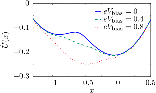
Figure 1: Resonant level. The shape of the effective potential $\tilde{U}(X)$ can be tuned by the bias voltage. We consider the parameters $eV_{\mathrm{gate}}=0$, $\hbar\omega_{0}=0.01$ and $\Gamma=0.1$. The dimensionless coordinate is $x=({M\omega_{0}^{2}}/{\lambda})X$ and energies are measured in units of ${\lambda^{2}}/{(M\omega_{0}^{2})}$.

Alternative expressions of the current-induced forces for the resonant level model, in terms of phase shifts and transmission coefficients, are given in the Supplementary Material C.

V.2 Two-level model

For the resonant level model discussed so far, the A-matrix vanishes and the damping is necessarily positive. We now consider a model which allows for negative damping [Metelmann and Brandes, 2011]. Our toy model could be inspired by a double dot on a suspended carbon nanotube, or an H₂ molecule in a break junction. The model is depicted schematically in Fig. 2. The bare dot Hamiltonian corresponds to degenerate electronic states $\epsilon_{0}$, localized on the left and right atoms or quantum dots, with tunnel coupling $t$ in between,

$$H_{0}=\left(\begin{array}[]{cc}\epsilon_{0}&t\\ t&\epsilon_{0}\end{array}\right)\,.$$ (76)

We consider a single oscillator mode with coordinate $X$ that couples linearly to the difference in the occupation of the levels. In our previous notation, this means $\Lambda_{1}=\lambda_{1}\sigma_{3}$, where we denote by $\sigma_{\mu}$, with $\mu=0,\ldots,3$, the Pauli matrices acting in the two-site basis. The shift of the electronic levels is given by $\tilde{\epsilon}_{\pm}(X)=\epsilon_{0}\pm\lambda_{1}X$.

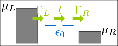
Figure 2: Sketch of the two-level model. Electrons tunnel through two degenerate energy levels between left and right leads. The system is modulated by the coupling to the vibrational modes.

The hybridization matrices are given by $\Gamma^{\alpha}=\frac{1}{2}\Gamma_{\alpha}(\sigma^{0}\pm\sigma^{3})$, where the $+(-)$ refers to $\alpha=L(R)$. We can deduce the tunneling matrix $W$ in terms of the hybridization matrices,

$$W=1/2\sqrt{\Gamma_{L}/\pi}(\sigma^{0}+\sigma^{3})+1/2\sqrt{\Gamma_{R}/\pi}(\sigma^{0}-\sigma^{3})\,.$$ (77)

In the wide-band limit, we approximate $W$ and $\Gamma_{\alpha}$ to be independent of energy. The retarded adiabatic GF takes the form

$$G^{R}(\epsilon,X)=\frac{1}{\Delta}\left(\begin{array}[]{cc}\epsilon-\tilde{\epsilon}_{+}+i\Gamma_{R}&t\\ t&\epsilon-\tilde{\epsilon}_{-}+i\Gamma_{L}\end{array}\right)\,,$$ (78)

with $\Delta(X)=\left(\epsilon-\tilde{\epsilon}_{-}+i\Gamma_{L})(\epsilon-\tilde{\epsilon}_{+}+i\Gamma_{R}\right)-t^{2}$.

For simplicity, we restrict our attention to symmetric couplings to the leads, $\Gamma_{L}=\Gamma_{R}=\Gamma/2$. Hence the frozen S-matrix $S(\epsilon,X)$ becomes

$$S(\epsilon,X)=1-\frac{i\Gamma}{\Delta}\left(\begin{array}[]{cc}\epsilon-\tilde{\epsilon}_{+}+i\Gamma/2&t\Gamma\\ t\Gamma&\epsilon-\tilde{\epsilon}_{-}+i\Gamma/2\end{array}\right)\,,$$ (79)

while the A-matrix takes the form

$$A(\epsilon,X)=i\lambda_{1}\Gamma\,t\,\frac{\left(\epsilon-\epsilon_{0}+i\Gamma/2\right)^{2}+i\left[(\lambda_{1}X)^{2}-t^{2}\right]}{\Delta^{3}}\,\sigma_{2}\,.$$ (80)

We can now give explicit expressions for the current-induced forces. The explicit expressions are lengthy and are given in Supp. Mat. D, Eqs. (116) and (D) for the mean force and damping matrix, respectively. The variance of the fluctuating force can be calculated accordingly.

The average force given in Eq. (116) of Supp. Mat. D combines with the elastic force to give rise to the effective potential $\tilde{U}(X)$ depicted, for zero temperature, in Fig. 3. As in the case studied in the previous section, the system can exhibit various levels of multistability when changing the bias.

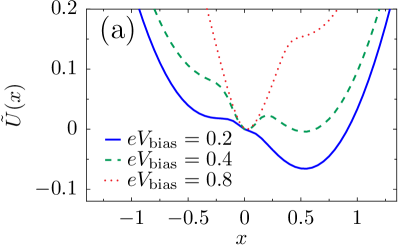
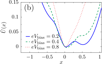
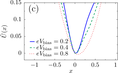
Figure 3: Effective potential for the mechanical motion in the two-level model. The shape of the potential can be tuned by changing the bias and gate voltages: (a) $eV_{\mathrm{gate}}=0$, (b) $eV_{\mathrm{gate}}=0.2$ and (c) $eV_{\mathrm{gate}}=0.4$. We consider the parameters $\hbar\omega_{0}=0.01$, $t=0.1$ and $\Gamma=0.1$. The dimensionless coordinate is $x=({M\omega_{0}^{2}}/{\lambda_{1}})X$ and energies are measured in units of ${\lambda_{1}^{2}}/{(M\omega_{0}^{2})}$.

The results for the friction coefficient, given in Supp. Mat. D Eq. (D), are shown in Fig. 4 as a function of the dimensionless oscillator coordinate $x$, for zero temperature. The contribution $\gamma^{s,eq}$ to the friction coefficient is peaked at $eV_{\mathrm{gate}}\pm eV_{\mathrm{bias}}/2=\pm\sqrt{(\lambda_{1}X)^{2}+t^{2}}$, as depicted in Figs. 4 (a) and (c). Neglecting the coupling to the leads, our toy model can be considered as a two-level system with level-spacing $2\sqrt{(\lambda_{1}X)^{2}+t^{2}}$. Thus, the peaks occur when one of the dot’s electronic levels enters the conduction window. When this happens, small changes in the oscillator coordinate $X$ can have a large impact on the occupation of the levels. This effect is more pronounced when the dots’ levels pass the Fermi levels that they are directly attached to [corresponding to $X>0$ for current flowing from left to right, see Fig. 4 (a) and Fig. 5 (a), (b)]. The broadening of the peaks is due to the hybridization with the leads, $\Gamma/2$. When $eV_{\mathrm{gate}}=0$, two peaks are expected symmetrically about $X=0$, as shown in Fig. 4 (a) [see also Figs. 5 (a) and (b)]. The effect of a finite gate voltage $eV_{\mathrm{gate}}$ is two-fold: it shifts the non-interacting electronic levels of the dot away from the middle of the conduction window, and hence the shifted levels $\tilde{\epsilon}_{\pm}$ pass the Fermi levels of right and left leads at different values of $X$, Figs. 5 (c) and (d). Therefore in this case four peaks are expected, with two larger peaks located at $X>0$, and two smaller peaks located at $X<0$. This is shown in Fig. 4 (c). The height of the peaks in this case is reduced with respect to the case $eV_{\mathrm{gate}}=0$, since for a given peak, only one of the dot’s levels is in resonance with one of the leads. Note that four real values of $X$ can be obtained only if $\left(eV_{\mathrm{gate}}\pm eV_{\mathrm{bias}}/2\right)^{2}>t^{2}$. A situation with $\left(eV_{\mathrm{gate}}-eV_{\mathrm{bias}}/2\right)^{2}<t^{2}$ while $\left(eV_{\mathrm{gate}}+eV_{\mathrm{bias}}/2\right)^{2}>t^{2}$ is shown in 4 (c) (red-dotted line), where a big peak is observed for $X=1/\lambda_{1}\sqrt{\left(eV_{\mathrm{gate}}+eV_{\mathrm{bias}}/2\right)^{2}-t^{2}}$, a corresponding small peak for $X=-1/\lambda_{1}\sqrt{\left(eV_{\mathrm{gate}}+eV_{\mathrm{bias}}/2\right)^{2}-t^{2}}$ [not displayed in Fig. 4 (c)], plus a peak at $X=0$.

For this model, the A-matrix is generally non-vanishing, which can result in negative damping for out-of-equilibrium situations. This is due to a negative contribution of $\gamma^{s,ne}$ to the total damping. This is visualized in Figs. 4 (b) and (d). Negative damping is possible when both dot levels are inside the conduction window, restricting the region in $X$ over which negative damping can occur. Indeed, when only one level is within the conduction window, the system effectively reduces to the resonant level model for which, as we showed in the previous subsection, the friction coefficient $\gamma^{s}$ is always positive. When current flows from left to right, negative damping occurs only for positive values of the oscillator coordinate $X$, as shown in Figs. 4 (b) and (d). This is consistent with a level-inversion picture, as discussed recently in Ref. [Lü et al., 2011]. Pictorially, the electron-vibron coupling causes a splitting in energy of the left and right levels. When $X>0$, electrons can go “down the ladder” formed by the energy levels by passing energy to the oscillator and hence amplifying the vibrations. For $X<0$, electrons can pass between the two dots only by absorbing energy from the vibrations, causing additional non-equilibrium damping. For small broadening of the dot levels due to the coupling to the leads, this effect is expected to be strongest when the vibration-induced splitting $\lambda_{1}X$ becomes of the same order as the strength of the hopping $t$. When $X$ grows further, the increasing detuning of the dot levels reduces the current and hence the non-equilibrium damping [see Figs. 4 (b) and (d) and Figs. 6 (a), (b)].

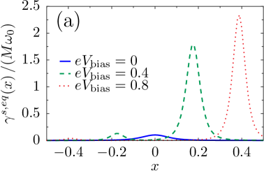
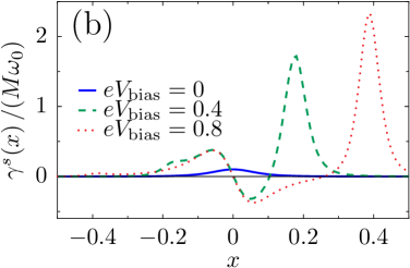
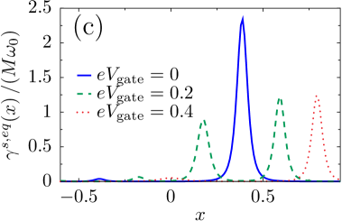
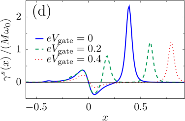
Figure 4: Damping vs. mechanical displacement in the two-level model. (a) Contribution $\gamma^{s,eq}$ to the friction coefficient for various bias voltages at fixed gate voltage $eV_{\mathrm{gate}}=0$. (b) At the same gate voltage, the total damping exhibits a region of negative damping due to the contribution of $\gamma^{s,ne}$. (c) $\gamma^{s,eq}$ for various gate voltages with the bias voltage $eV_{\mathrm{bias}}=0.8$. Note that for both $eV_{\mathrm{gate}}=0.2$ and $eV_{\mathrm{gate}}=0.4$, one small peak for negative $x$ falls outside of the shown range of $x$. (d) Again, the full damping $\gamma^{s}$ exhibits regions of negative damping. We choose $\hbar\omega_{0}=0.01$, $\Gamma=0.1$ and $t=0.1$. The dimensionless coordinate is $x=({M\omega_{0}^{2}}/{\lambda_{1}})X$ and energies are measured in units of ${\lambda_{1}^{2}}/{(M\omega_{0}^{2})}$.

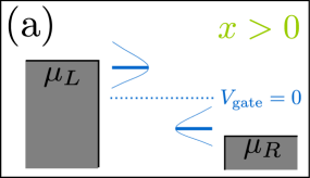
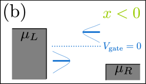
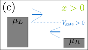
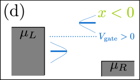
Figure 5: Cartoon of the positions of the electronic levels in the dot with respect to the Fermi levels of the leads, depending on the sign of $x$ and the existence of a gate voltage. The levels are broadened due to the hybridization with the leads $\Gamma$. When $x>0$, “left” and “right” levels approach the Fermi levels of left and right leads respectively, (a) for $eV_{\mathrm{gate}}=0$ the levels align simultaneously for left and right, (c) a finite $eV_{\mathrm{gate}}$ produces an assymmetry between left and right. For $x<0$ the alignment of the levels is inverted, (b) $eV_{\mathrm{gate}}=0$, (d) finite $eV_{\mathrm{gate}}$.

The coexistence of a multistable potential together with regions of negative damping can lead to interesting nonlinear behavior for the dynamics of the oscillator. In particular, and as we show in the next example, limit-cycle solutions are possible, in the spirit of a Van der Pol oscillator [Hanggi and Riseborough, 1983].

We can also calculate the current. The pumping contribution is proportional to the velocity $\dot{X}$ and thus small. Therefore we show here results only for the dominant adiabatic part of the current. This is given by

$$I^{0}=\frac{e}{h}\int d\epsilon\frac{2t^{2}\Gamma^{2}(f_{L}-f_{R})}{\left|\Delta\right|^{2}}\,.$$ (81)

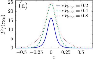
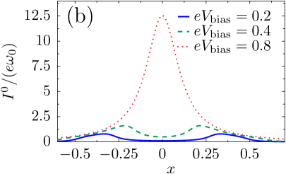
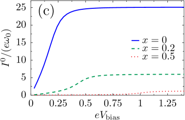
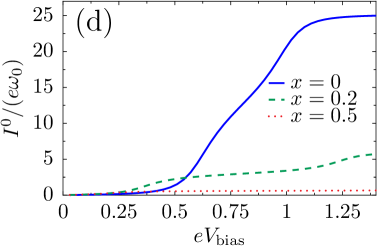
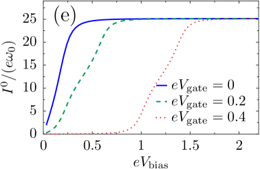
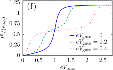
Figure 6: Dependence of the current in the two-level model on various parameters. Current as function of mechanical displacement for (a) $V_{\mathrm{gate}}=0$ and (b) $V_{\mathrm{gate}}=0.4$; as function of bias for (c) $V_{\mathrm{gate}}=0$, (d) $V_{\mathrm{gate}}=0.4$, (e) $x=0$ and (f) $x=0.5$. We choose $\hbar\omega_{0}=0.01$, $\Gamma=0.1$ and $t=0.1$. The dimensionless coordinate is $x=({M\omega_{0}^{2}}/{\lambda_{1}})X$ and energies are measured in units of ${\lambda_{1}^{2}}/{(M\omega_{0}^{2})}$.

For zero temperature, the behavior of the current is shown in Fig. 6 as a function of various parameters. Figs. 6 (a) and (b) show the current as a function of the (dimensionless) oscillator coordinate $x$ for two different values of gate potential for which the system exhibits multistability by developing several metastable equilibrium positions. For $V_{\mathrm{gate}}=0$ and independently of bias, the current shows a maximum at the local minimum of the effective potential $x=0$, while $I^{0}\approx 0$ for another possible local minimum, $x\approx 0.5$ (compare with Fig. 3 (a)). The true equilibrium value of $x$ can be tuned via the bias potential, showing the possibility of perfect switching. For finite gate potential however, the current is depleted from $x=0$ with diminishing bias. Figs. 6 (c) to (d) show the current as a function of gate or bias voltage for fixed representative values of the oscillator coordinate $x$. The current changes stepwise as the number of levels inside the conduction window changes, coinciding with the peaks in the friction coefficient illustrated in Fig. 4. In an experimental setting, the measured dc current would involve an average over the probability distribution of the coordinate $x$, given by the solution of the Fokker-Planck equation associated to the Langevin equation (1).

V.3 Two vibrational modes

As a final example, we present a simple model which allows for both a non-conservative force and an effective “Lorentz” force, in addition to negative damping. For this it is necessary to couple the two electronic orbitals of the previous example, see Eq. (76), to at least two oscillatory modes which we assume to be degenerate. The relevant vibrations in this case can be thought of as a center-of-mass vibration $X_{1}$ between the leads, and a stretching mode $X_{2}$. (It should be noted that this is for visualization purposes only. In reality, for an H₂ molecule, the stretching mode is a high energy mode when compared to a transverse and a rotational mode, see Ref. [Djukic et al., 2005]. Nevertheless, the H₂ molecule does indeed have two near-degenerate low energy vibrational modes, corresponding to rigid vibrations between the leads and a rigid rotation relative to the axis defined by the two leads.) The stretch mode modulates the hopping parameter,

$$t\to\tilde{t}(X_{2})=t+\lambda_{2}X_{2}\,,$$ (82)

while the center of mass mode $X_{1}$ is modeled as coupling linearly to the density,

$$\epsilon_{0}\to\tilde{\epsilon}(X_{1})=\epsilon_{0}+\lambda_{1}X_{1}\,,$$ (83)

hence $\Lambda_{1}=\lambda_{1}\sigma_{0}$ and $\Lambda_{2}=\lambda_{2}\sigma_{1}$. We work in the wide-band limit, but allow for asymmetric coupling to the leads. The retarded Green’s function becomes

$$G^{R}(\epsilon,X_{1},X_{2})=\frac{1}{\Delta}\left(\begin{array}[]{cc}\epsilon-\tilde{\epsilon}+i\Gamma_{R}&\tilde{t}\\ \tilde{t}&\epsilon-\tilde{\epsilon}+i\Gamma_{L}\end{array}\right)\,,$$ (84)

where now $\Delta(X_{1},X_{2})=(\epsilon-\tilde{\epsilon}+i\Gamma_{L})(\epsilon-\tilde{\epsilon}+i\Gamma_{R})-\tilde{t}^{2}$. The frozen S-matrix can be easily calculated to be

$$S(\epsilon,X_{1},X_{2})=1-\frac{2i}{\Delta}\left(\begin{array}[]{cc}\left(\epsilon-\tilde{\epsilon}+i\Gamma_{R}\right)\Gamma_{L}&\tilde{t}\sqrt{\Gamma_{L}\Gamma_{R}}\\ \tilde{t}\sqrt{\Gamma_{L}\Gamma_{R}}&\left(\epsilon-\tilde{\epsilon}+i\Gamma_{L}\right)\Gamma_{R}\end{array}\right)\,.$$ (85)

The A-matrices also take a simple form for this model. Since $\Lambda_{1}$ is proportional to the identity operator,

$$A_{1}(\epsilon,X_{1},X_{2})=-\pi\lambda_{1}\,WG_{R}\,[G_{R},\sigma_{0}]\,G_{R}W^{\dagger}=0\,.$$ (86)

On the other hand, the A-matrix associated with $X_{2}$ is non-zero and given by

$$A_{2}(\epsilon,X_{1},X_{2})=-i\lambda_{2}\,\frac{\sqrt{\Gamma_{1}\Gamma_{2}}}{\Delta^{2}}\,\sigma_{2}\,.$$ (87)

From this we can compute the average force, damping, pseudo-Lorentz force, and noise terms. These are listed in Supp. Mat. E. At zero temperature, it is possible to obtain analytical expressions for these current-induced forces. Studying the dynamics of the modes $X_{1,2}(t)$ implies solving the two coupled Langevin equations given by Eq. (1), after inserting the expressions for the forces given in Supp. Mat. E. Within our formalism we are able to study the full non-linear dynamics of the problem, which brings out a plethora of new qualitative behavior. In particular, analyses which linearize the current-induced force about a static equilibrium point would predict run-away modes due to negative damping and non-conservative forces [Lü et al., 2010]. Taking into account nonlinearities allows one to find the new stable attractor of the motion. Indeed, we find that these linear instabilities typically result in dynamical equilibrium, namely limit-cycle dynamics [Bode et al., 2011]. We note in passing that limit cycle dynamics in a nanoelectromechanical system was also discussed recently in Ref.  [Metelmann and Brandes, 2011].

We have studied the zero-temperature dynamics of our two-level, two-mode system for different ranges of parameters. In Fig. (7) we map out the values of the curl of the mean force, $\left(\nabla\times F\right)_{\perp}$, indicating that the force is non-conservative throughout parameter space. We also plot one of the two eigenvalues of the dissipation matrix $\gamma^{s}$, showing that it can take negative values in some regions of the parameter space. We find that it is possible to drive the system into a limit cycle by varying the bias potential. The existence of this limit cycle is shown in Fig. 8 (a), where we have plotted various Poincaré sections of the non-linear system without fluctuations. The figure shows the trajectory in phase space of the (dimensionless) oscillator coordinate $x_{1}$ after the dynamical equilibrium is reached, for several cuts of the (dimensionless) coordinate $x_{2}$. Each cut shows two points in $x_{1}$ phase space, indicating the entry and exit of the trajectory. Each point in the plot actually consists of several points that fall on top of each other, corresponding to every time the coordinate $x_{2}$ has the value indicated in the legend of Fig. 8 (a). This shows the periodicity of the solution of the non-linear equations of motion for $x_{1},\,x_{2}$ for the particular bias chosen. Surveying over the various values of $x_{2}$ reveals a closed trajectory in the parametric coordinate space $x_{1},\,x_{2}$.

Remarkably, signatures of the limit cycle survive the inclusion of the Langevin force. Fig. 8 (b) depicts typical trajectories in the oscillator’s coordinate space $x_{1},\,x_{2}$ in the presence of the stochastic force, showing fluctuating trajectories around the stable limit cycle.

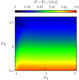
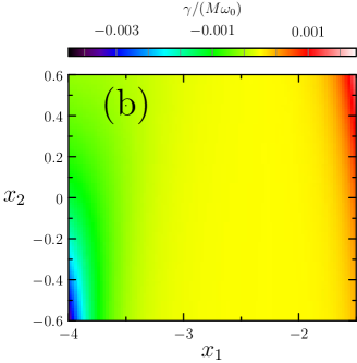
Figure 7: Curl of the average force and damping coefficient for the model with two vibrational modes: (a) The curl of the current-induced mean force ${\mathbf{F}}$ is, in a non-equilibrium situation, generally non-zero, indicating that the force is non-conservative. (b) One of the two eigenvalues of $\gamma^{s}$. Remarkably, it undergoes sign changes. A dissipation matrix $\gamma^{s}$ which is non-positive definite implies destabilization of the static equilibrium solution found at lower bias potentials, in this case driving the system into a limit cycle, see main text and Fig. 8. The parameters used are such that $\lambda_{1}/\lambda_{2}=3/2$. The elastic modes are degenerate with $\hbar\omega_{0}=0.014$, $\Gamma_{L,R}=\frac{1\pm 0.8}{2}(\sigma_{0}\pm\sigma_{z})$, and the hopping between the orbitals is $t=0.9$. The dimensionless coordinates are $x_{i}=({M\omega_{0}^{2}}/{\lambda})X_{i}$ and energies are in units of ${\lambda^{2}}/{(M\omega_{0}^{2})}$, where $\lambda=({\lambda_{1}+\lambda_{2}})/{2}$.

$\begin{array}[]{cccc}\includegraphics[height=113.81102pt,keepaspectratio={true}]{xxdot-01.pdf}&\includegraphics[height=113.81102pt,keepaspectratio={true}]{x1x2-01.pdf}\end{array}$

Figure 8: Limit-cycle dynamics for the model with two vibrational modes. (a) At large bias voltages, Poincaré sections of the four dimensional phase space show the presence of a limit cycle in the Langevin dynamics without fluctuating force. (b) Several periods of typical trajectories (for different initial conditions after a transient) in the presence of the fluctuating forces ${\mathbf{\xi}}$ are shown. The same general parameters as in Fig. 7 are used here.

Experimentally, the signature of the limit cycle would be most directly reflected in the current-current correlation function, as depicted in Fig. 9. We find that in the absence of a limit cycle the system is dominated by two characteristic frequencies, shown by the peaks in Fig. 9. These frequencies correspond to the shift in energy of the two degenerate vibrational modes due to the average current-induced forces $F_{1}$ and $F_{2}$. When the bias voltage is such that the system enters a limit cycle, the current-current correlation shows instead only one peak as a function of frequency. This result, as shown in Fig. 9, is fairly robust to noise, making the onset of limit-cycle dynamics observable in experiment.

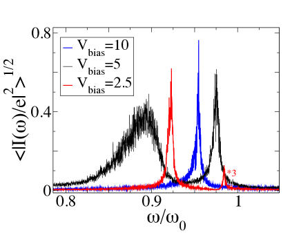
Figure 9: Current-current correlation function in the presence of noise for the system with two vibrational modes. The limit cycle is signaled by a single peak ($V_{bias}=10$, see Fig. 8), as opposed to two peaks in the absence of a limit cycle ($V_{bias}=2.5,\,5$). Increasing the bias potential increases the noise levels but the peaks are still easily recognizable. The results are obtained by averaging over times long enough compared with the characteristic oscillation times. The same general parameters as in Fig. 7 are used here.

VI Conclusions

Within a non-equilibrium Born-Oppenheimer approximation, the dynamics of a nanoelectromechanical system can be described in terms of a Langevin equation, in which the mechanical modes of the mesoscopic device are subject to current-induced forces. These forces include a mean force, which is independent of velocity and due to the average net force the electrons exert on the oscillator, a stochastic Langevin force which takes into account the thermal and non-equilibrium fluctuations with respect to the mean force value, and a force linear in the velocity of the modes. This last, velocity dependent force, consists of a dissipative term plus a term that can be interpreted as an effective “Lorentz” force, due to an effective magnetic field acting in the parameter space of the modes.

In this work we have expressed these current-induced forces through the scattering matrix of the coherent mesoscopic conductor and its parametric derivatives, extending the results found previously in Ref. [Bode et al., 2011]. Our results are now valid for a generic coupling between the electrons and the vibrational degrees of freedom, given by a matrix $h_{0}(\mathbf{X})$, and for energy-dependent hybridization with the leads, given by the matrix $W(\epsilon)$. We have shown that expressing all the current-induced forces in terms of the S-matrix is only possible by going beyond the strictly adiabatic approximation, and it is necessary to include the first order correction in the adiabatic expansion. This introduces a new fundamental quantity into the problem, the A-matrix, which needs to be calculated together with the frozen S-matrix for a given system.

There are several circumstances in which the first non-adiabatic correction, encapsulated in the A-matrix, is necessary. While the average as well as the fluctuating force can be expressed solely in terms of the adiabatic S-matrix, the A-matrix enters both the frictional and the Lorentz-like force. In equilibrium, the frictional force reduces to an expression in terms of the adiabatic S-matrix. Out of equilibrium, however, an important new contribution involving the A-matrix appears. In contrast, the A-matrix is always required to express the Lorentz-like force, even when the system is in thermal equilibrium.

The expressions for the current-induced forces in terms of the scattering matrix allow us to extract important properties from general symmetry arguments. Driving the nanoelectromechanical system out of equilibrium by imposing a bias results in qualitatively new features for the forces. We have shown that the mean force is non-conservative in this case, and that the dissipation coefficient acquires a non-equilibrium contribution that can be negative. We have also shown that when considering more than one mechanical degree of freedom, a pseudo Lorentz force is present even for a time-reversal invariant system, unless one also imposes thermal equilibrium on top of the time-reversal condition.

Our model allows one to study, within a controlled approximation, the non-linear dynamics generated by the interplay between current and vibrational degrees of freedom, opening up the path for a systematic study of these devices. By means of simple model examples, we have shown that it is possible to drive a nanoelectromechanical system into interesting dynamically stable regimes such as a limit cycle, by varying the applied bias potential. In a limit cycle, the vibrational modes vary periodically in time, which can be the operating principle for a molecular motor. On the other hand, the possibility of non-conservative forces could also allow one to extract energy from the system, providing a controllable tool for cooling. The study of these kinds of phenomena for realistic systems is an interesting application of the formalism presented in this paper.

VII Acknowledgments

We acknowledge discussions with P. W. Brouwer, G. Zarand, and L. Arrachea as well as support by the DFG through SPP 1459, SFB TR/12, and SFB 658.

Appendix A Useful relations

Here we list a set of useful relations for the derivations in the main text.

A.1 Green’s functions relations

The Green’s functions are related via

$$G^{R}-G^{A}=G^{>}-G^{<}.$$ (88)

The lesser and larger Green’s functions are given by

$$G^{<} =G^{R}\Sigma^{<}G^{A}=2i\sum_{\alpha}f_{\alpha}\,G^{R}\Gamma_{\alpha}G^{A}=2\pi i\sum_{\alpha}f_{\alpha}\,G^{R}W^{\dagger}\Pi_{\alpha}WG^{A}$$ (89)

$$G^{>} =G^{<}+G^{R}-G^{A}=-2\pi i\sum_{\alpha}(1-f_{\alpha})\,G^{R}W^{\dagger}\Pi_{\alpha}WG^{A}.$$ (90)

From (22) it is easy to see that

$$W^{\dagger}W=\frac{1}{2\pi i}[(G^{R})^{-1}-(G^{A})^{-1}]\,,$$ (91)

$$\partial_{X_{\nu}}G^{R}=G^{R}\Lambda_{\nu}G^{R}$$ (92)

and

$$\partial_{\epsilon}G^{R}=-G^{R}(1-\partial_{\epsilon}\Sigma^{R})G^{R}.$$ (93)

A.2 Green’s functions and S-matrix relations

Noting that (for given $t$) $\partial_{X_{\nu}}G^{R}=G^{R}\Lambda_{\nu}G^{R}$, we find using Eq.(91):

$$S^{\dagger}\frac{\partial S}{\partial X_{\nu}}=-2\pi i(1+2\pi iWG^{A}W^{\dagger})WG^{R}\Lambda_{\nu}G^{R}W^{\dagger}=-2\pi iWG^{A}\Lambda_{\nu}G^{R}W^{\dagger}.$$ (94)

This holds for arbitrary magnitude of $X_{\nu}$.

In the main text we use

$$\frac{1}{\pi}\frac{\partial S^{\dagger}}{\partial X_{\nu}}A_{\nu^{\prime}}=2\pi iWG^{A}\Lambda_{\nu}G^{A}W^{\dagger}\partial_{\epsilon}(WG^{R})\Lambda_{\nu^{\prime}}G^{R}W^{\dagger}-WG^{A}\Lambda_{\nu}(G^{A}-G^{R})\Lambda_{\nu^{\prime}}\partial_{\epsilon}(G^{R}W^{\dagger}),$$ (95)

$$\pi\left(\left[S^{\dagger}\frac{\partial S}{\partial X_{\nu}},WG^{A}\Lambda_{\nu^{\prime}}\frac{\partial(G^{R}W^{\dagger})}{\partial_{\epsilon}}-\frac{\partial(WG^{A})}{\partial_{\epsilon}}\Lambda_{\nu^{\prime}}G^{R}W^{\dagger}\right]_{-}\right)_{s}=\left(\frac{\partial S^{\dagger}}{\partial X_{\nu}}A_{\nu^{\prime}}-A^{\dagger}_{\nu^{\prime}}\frac{\partial S}{\partial X_{\nu}}\right)_{s}$$ (96)

and

$$\left[S^{\dagger}\frac{\partial A_{\nu}}{\partial X_{\nu^{\prime}}}\right]_{a}=-2\pi\left[WG^{A}\Lambda_{\nu}(\partial_{\epsilon}G^{R})\Lambda_{\nu^{\prime}}G^{R}W^{\dagger}\right]_{a}.$$ (97)

For energy-independent $\Gamma^{\alpha}$, we can use (93) so that also

$$S^{\dagger}\frac{\partial S}{\partial\epsilon}=2\pi iWG^{A}G^{R}W^{\dagger},$$ (98)

$$\partial_{\epsilon}\left(S^{\dagger}\frac{\partial S}{\partial X_{\nu}}\right) =2\pi iWG^{A}\left(G^{A}\Lambda_{\nu}+\Lambda_{\nu}G^{R}\right)G^{R}W^{\dagger}$$ (99)

and (95) simplifies to

$$\frac{\partial S^{\dagger}}{\partial X_{\nu}}A_{\nu^{\prime}}=\pi WG^{A}\Lambda_{\nu}\left(G^{A}-G^{R}\right)\left(\Lambda_{\nu^{\prime}}G^{R}-G^{R}\Lambda_{\nu^{\prime}}\right)G^{R}W^{\dagger}.$$ (100)

Appendix B S-matrix derivation of the damping matrix

The expression for $\gamma^{s}$ given in Eq. (27) can be written explicitly in terms of retarded and advanced Green’s functions as

$$\gamma^{s}_{\nu\nu^{\prime}}=2\pi\sum_{\alpha\alpha^{\prime}}\int d\epsilon f_{\alpha}{\rm tr}\left\{\Lambda_{\nu}G^{R}W^{\dagger}\Pi_{\alpha}WG^{A}\Lambda_{\nu^{\prime}}\partial_{\epsilon}\left[(1-f_{\alpha^{\prime}})G^{R}W^{\dagger}\Pi_{\alpha^{\prime}}WG^{A}\right]\right\}_{s}\,.$$ (101)

We split Eq. (101) into two terms, the first due to the derivative acting on the Fermi function, the second from the rest, $\gamma^{s}=\gamma^{s(I)}+\gamma^{s(II)}$. The first term is given by

$$\gamma^{s(I)}_{\nu\nu^{\prime}}=2\pi\sum_{\alpha\alpha^{\prime}}\int d\epsilon f_{\alpha}(-\partial_{\epsilon}f_{\alpha^{\prime}}){\rm tr}\left\{\Pi_{\alpha^{\prime}}WG^{A}\Lambda_{\nu}G^{R}W^{\dagger}\Pi_{\alpha}WG^{A}\Lambda_{\nu^{\prime}}G^{R}W^{\dagger}\right\}_{s}$$ (102)

where we have used the cyclic invariance of the trace. Similar to the derivation for the mean force, by means of expression (94) in Supp. Mat. A, Eq. (102) can be expressed in terms of the frozen S-matrix as

$$\gamma^{s(I)}_{\nu\nu^{\prime}}=-\sum_{\alpha\alpha^{\prime}}\int\frac{\rm d\epsilon}{2\pi}f_{\alpha}(-\partial_{\epsilon}f_{\alpha^{\prime}}){\rm Tr}\left\{\Pi_{\alpha}S^{\dagger}\frac{\partial S}{\partial X_{\nu}}\Pi_{\alpha^{\prime}}S^{\dagger}\frac{\partial S}{\partial X_{\nu^{\prime}}}\right\}_{s}\,.$$ (103)

The second contribution, in terms of $G^{R}$ and $G^{A}$, reads

$$\gamma^{s(II)}_{\nu\nu^{\prime}}=(2\pi)^{2}\sum_{\alpha\alpha^{\prime}}\int\frac{{\rm d}\epsilon}{2\pi}F_{\alpha\alpha^{\prime}}{\rm tr}\left\{\Lambda_{\nu}G^{R}W^{\dagger}\Pi_{\alpha}WG^{A}\Lambda_{\nu^{\prime}}\partial_{\epsilon}\left(G^{R}W^{\dagger}\Pi_{\alpha^{\prime}}WG^{A}\right)\right\}_{s}\,.$$ (104)

It is instructive to split the factor $F_{\alpha\alpha^{\prime}}$ into a symmetric and an antisymmetric part under exchange of the lead indices, $F_{\alpha\alpha^{\prime}}=F^{s}_{\alpha\alpha^{\prime}}+F^{a}_{\alpha\alpha^{\prime}}$, with

$$\begin{split}F^{s}_{\alpha\alpha^{\prime}}&\equiv\frac{1}{2}(f_{\alpha}+f_{\alpha^{\prime}}-2f_{\alpha}f_{\alpha^{\prime}})\\ F^{a}_{\alpha\alpha^{\prime}}&\equiv\frac{1}{2}(f_{\alpha}-f_{\alpha^{\prime}})\,.\end{split}$$ (105)

Correspondingly, we split $\gamma^{s(II)}$ into symmetric $\left[\gamma^{s(IIs)}\right]$ and antisymmetric $\left[\gamma^{s(IIa)}\right]$ parts in the lead indices: $\gamma^{s(II)}=\gamma^{s(IIs)}+\gamma^{s(IIa)}$. Due to its symmetries, $\gamma^{s(IIs)}$ can be easily expressed in terms of the S-matrix,

$$\begin{split}\gamma^{s(IIs)}_{\nu\nu^{\prime}}&=\pi\sum_{\alpha\alpha^{\prime}}\int d\epsilon F^{s}_{\alpha\alpha^{\prime}}\partial_{\epsilon}{\rm tr}\left\{\Lambda_{\nu}G^{R}W^{\dagger}\Pi_{\alpha}WG^{A}\Lambda_{\nu^{\prime}}G^{R}W^{\dagger}\Pi_{\alpha^{\prime}}WG^{A}\right\}_{s}\\ &=-\pi\sum_{\alpha\alpha^{\prime}}\int d\epsilon\left(\partial_{\epsilon}F^{s}_{\alpha\alpha^{\prime}}\right){\rm tr}\left\{\Lambda_{\nu}G^{R}W^{\dagger}\Pi_{\alpha}WG^{A}\Lambda_{\nu^{\prime}}G^{R}W^{\dagger}\Pi_{\alpha^{\prime}}WG^{A}\right\}_{s}\\ &=\frac{1}{4\pi}\sum_{\alpha\alpha^{\prime}}\int d\epsilon\left(\partial_{\epsilon}F^{s}_{\alpha\alpha^{\prime}}\right){\rm tr}\left\{\Pi_{\alpha}S^{\dagger}\frac{\partial S}{\partial X_{\nu}}\Pi_{\alpha^{\prime}}S^{\dagger}\frac{\partial S}{\partial X_{\nu^{\prime}}}\right\}_{s}\end{split}$$ (106)

where in the second line we have integrated by parts since $F^{s}$ vanishes for $\epsilon\to\pm\infty$, and in the last line we have used Eq. (94) from App. A once again.

B.1 “Equilibrium” dissipative term $\gamma^{s,eq}$

Since in equilibrium $F^{a}_{\alpha\alpha^{\prime}}=F^{a}_{\alpha\alpha}=0$, $\left.\gamma^{s(IIa)}\right|_{eq}=0$ and we can now regroup terms into an “equilibrium” contribution, $\gamma^{s,eq}=\gamma^{s(I)}+\gamma^{s(IIs)}$, and a purely non-equilibrium contribution $\gamma^{s,ne}\equiv\gamma^{s(IIa)}$:

$$\gamma^{s}=\gamma^{s,eq}+\gamma^{s,ne}\,.$$ (107)

By adding up expressions (103) and (106), it is straightforward to obtain Eq. (44) for $\gamma^{s,eq}$ given in the main text.

B.2 Non-equilibrium dissipative term $\gamma^{s,ne}$

To obtain $\gamma^{s,ne}$ in terms of S-matrix quantities we start from the expression

$$\gamma^{s,ne}_{\nu\nu^{\prime}}=2\pi\sum_{\alpha\alpha^{\prime}}\int{\rm d}\epsilon F_{\alpha\alpha^{\prime}}^{a}{\rm tr}\left\{\Lambda_{\nu}G^{R}W^{\dagger}\Pi_{\alpha}WG^{A}\Lambda_{\nu^{\prime}}\partial_{\epsilon}\left(G^{R}W^{\dagger}\Pi_{\alpha^{\prime}}WG^{A}\right)\right\}_{s}\,,$$ (108)

and exploiting $\sum_{\alpha}\Pi_{\alpha}=1$ and the identity (94) in Supp. Mat. A, we note that Eq. (108) can be written as

$$\gamma^{s,ne}_{\nu\nu^{\prime}}=-\frac{i}{2}\int{\rm d}\epsilon\sum_{\alpha}f_{\alpha}{\rm tr}\left\{\Pi_{\alpha}\left[S^{\dagger}\frac{\partial S}{\partial X_{\nu}},WG^{A}\Lambda_{\nu^{\prime}}\frac{\partial(G^{R}W^{\dagger})}{\partial\epsilon}-\frac{\partial(WG^{A})}{\partial\epsilon}\Lambda_{\nu^{\prime}}G^{R}W^{\dagger}\right]\right\}_{s}\,,$$ (109)

where $[.\,,\,.]$ indicates the commutator. Calculating each term in the commutator separately we obtain

$$\begin{split}S^{\dagger}\frac{\partial S}{\partial X_{\nu}}\left[WG^{A}\Lambda_{\nu^{\prime}}\frac{\partial(G^{R}W^{\dagger})}{\partial\epsilon}-\frac{\partial(WG^{A})}{\partial\epsilon}\Lambda_{\nu^{\prime}}G^{R}W^{\dagger}\right]&=-WG^{A}\Lambda_{\nu}(G^{A}-G^{R})\Lambda_{\nu^{\prime}}\frac{\partial(G^{R}W^{\dagger})}{\partial\epsilon}\\ &+2\pi iWG^{A}\Lambda_{\nu}G^{R}W^{\dagger}\frac{\partial(WG^{A})}{\partial\epsilon}\Lambda_{\nu^{\prime}}G^{R}W^{\dagger}\\ \left[WG^{A}\Lambda_{\nu^{\prime}}\frac{\partial(G^{R}W^{\dagger})}{\partial\epsilon}-\frac{\partial(WG^{A})}{\partial\epsilon}\Lambda_{\nu^{\prime}}G^{R}W^{\dagger}\right]S^{\dagger}\frac{\partial S}{\partial X_{\nu}}&=-\frac{\partial(WG^{A})}{\partial\epsilon}\Lambda_{\nu^{\prime}}(G^{A}-G^{R})\Lambda_{\nu}G^{R}W^{\dagger}\\ &-2\pi iWG^{A}\Lambda_{\nu^{\prime}}\frac{\partial(G^{R}W^{\dagger})}{\partial\epsilon}WG^{A}\Lambda_{\nu}G^{R}W^{\dagger}\,,\end{split}$$ (110)

where we have used Eq. (91) from Supp. Mat. A. Finally, with help of the identity (95) in Supp. Mat. A, the non-equilibrium term can be expressed as Eq. (45) in the main text.

Appendix C Resonant level forces: alternative expressions

To calculate the current-induced forces for the resonant level model presented in Sec. V, we can alternatively start with the popular S-matrix parametrization  [Nazarov and Blanter, 2010; Bennett et al., 2010]

$$S=\left(\begin{array}[]{cc}\sqrt{1-{\cal T}}e^{i\theta}&\sqrt{{\cal T}}e^{i\eta}\\ \sqrt{{\cal T}}e^{i\eta}&-\sqrt{1-{\cal T}}e^{i(2\eta-\theta)}\end{array}\right)\,,$$ (111)

where the transmission coefficient ${\cal T}$ and the phases $\eta,\theta$ depend on $X$. We present here the results for linear coupling, $\tilde{\epsilon}(X)=\epsilon_{0}+\lambda X$. We can then identify the transmission probability

$${\cal T}(\epsilon,X)=\frac{4\Gamma_{L}\Gamma_{R}}{(\epsilon-\epsilon_{0}-\lambda X)^{2}+\Gamma^{2}}$$ (112)

and the phases

$$\eta(\epsilon,X) = -\frac{\pi}{2}-\arctan\left(\frac{\Gamma}{\epsilon-\epsilon_{0}-\lambda X}\right)$$

$$\theta(\epsilon,X) = \frac{\pi}{2}+\eta+\arctan\left(\frac{\Gamma_{R}-\Gamma_{L}}{\epsilon-\epsilon_{0}-\lambda X}\right)\,.$$

We can now relate the current-induced forces to this S-matrix parametrization. The result for the average force can be split into a non-equilibrium force $F^{ne}$ and an equilibrium force $F^{eq}$, i.e., $F=F^{ne}+F^{eq}$ with

$$F^{ne}(X) = \int\frac{d\epsilon}{2\pi}(f_{L}-f_{R})(1-{\cal T})\frac{\partial(\theta-\eta)}{\partial X}$$ (113)

$$F^{eq}(X) = \int\frac{d\epsilon}{2\pi}(f_{L}+f_{R})\frac{\partial\eta}{\partial X}\,.$$

The amplitude of the fluctuating force can be obtained from Eq. (42) and is given by

$$D(X)=\int\frac{d\epsilon}{2\pi}\sum_{\alpha\alpha^{\prime}}F^{s}_{\alpha\alpha^{\prime}}Y_{\alpha\alpha^{\prime}}\,,$$ (114)

where we have defined

$$Y_{LL} = \left[(1-{\cal T})\frac{\partial(\eta-\theta)}{\partial X}-\frac{\partial\eta}{\partial X}\right]^{2}$$

$$Y_{RR} = \left[(1-{\cal T})\frac{\partial(\eta-\theta)}{\partial X}+\frac{\partial\eta}{\partial X}\right]^{2}$$

$$Y_{LR} = Y_{RL}=\frac{1}{4{\cal T}(1-{\cal T})}\left(\frac{\partial{\cal T}}{\partial X}\right)^{2}+{\cal T}(1-{\cal T})\left(\frac{\partial(\eta-\theta)}{\partial X}\right)^{2}.$$

After some algebra, we also obtain

$$\gamma^{s}(X)=\frac{1}{2T}\left[D(X)-\int\frac{d\epsilon}{2\pi}(f_{L}-f_{R})^{2}Y_{LR}\right]\,.$$ (115)

This last expression corresponds to $\gamma^{s,eq}$ given in Eq. (44). (As we pointed out previously, $\gamma^{s,ne}$ vanishes in this case). Here we have isolated a term that vanishes in equilibrium, showing explicitly that there is a non-equilibrium contribution in (44).

Appendix D Current-induced forces for the two-level model

The mean force is given by

$$F(X)=-\lambda_{1}\Gamma\int\frac{d\epsilon}{2\pi}\left[(f_{L}+f_{R})\frac{2\lambda_{1}X(\epsilon-\epsilon_{0})}{\left|\Delta\right|^{2}}+(f_{L}-f_{R})\frac{(\epsilon-\epsilon_{0})^{2}+(\lambda_{1}X)^{2}-t^{2}+(\Gamma/2)^{2}}{\left|\Delta\right|^{2}}\right]\,.$$ (116)

The friction coefficient $\gamma^{s}=\gamma^{s,eq}+\gamma^{s,ne}$ reads

$$\gamma^{s,eq}= \frac{\lambda_{1}^{2}\Gamma^{2}}{4\pi}\int d\epsilon\left\{-\frac{\partial_{\epsilon}f_{L}+\partial_{\epsilon}f_{R}}{\left|\Delta\right|^{4}}\Bigl{[}\left((\epsilon-\epsilon_{0})^{2}+(\Gamma/2)^{2}+(\lambda_{1}X)^{2}+t^{2}\right)^{2}+\left(2(\epsilon-\epsilon_{0})\lambda_{1}X\right)^{2}\right.$$

$$- \left.\left(2(\epsilon-\epsilon_{0})t\right)^{2}\Bigr{]}+\frac{\partial_{\epsilon}f_{R}-\partial_{\epsilon}f_{L}}{\left|\Delta\right|^{4}}\left[4(\epsilon-\epsilon_{0})\lambda_{1}X\left((\epsilon-\epsilon_{0})^{2}+(\Gamma/2)^{2}+(\lambda_{1}X)^{2}-t^{2}\right)\right]\right\}\,,$$

$$\gamma^{s,ne}= \frac{2\lambda_{1}^{2}\Gamma^{2}t^{2}\lambda_{1}X}{\pi}\int d\epsilon\,\frac{f_{R}-f_{L}}{\left|\Delta\right|^{6}}\Bigr{[}\left((\epsilon-\epsilon_{0})^{2}-(\lambda_{1}X)^{2}-t^{2}\right)^{2}$$

$$+ 2(\Gamma/2)^{2}\left((\epsilon-\epsilon_{0})^{2}+(\lambda_{1}X)^{2}+t^{2}\right)+(\Gamma/2)^{4}\Bigl{]}\,.$$ (117)

Appendix E Current-induced forces for the two vibrational modes model

Here we list the current-induced forces quantities, calculated from Eqs. (39), (42), (47) and (50) for the two-modes example discussed in the main text. For convenience, we define the following quantities:

$$g_{\alpha 0}(\epsilon) = \frac{(\epsilon-\tilde{\epsilon})^{2}+\tilde{t}^{2}+\Gamma_{1-\alpha}^{2}}{\left|\Delta\right|^{2}}$$ (118)

$$g_{\alpha 1}(\epsilon) = \frac{2\tilde{t}\,(\epsilon-\tilde{\epsilon})}{\left|\Delta\right|^{2}}$$ (119)

$$g_{\alpha 2}(\epsilon) = \pm\frac{-2\tilde{t}\,\Gamma_{1-\alpha}}{\left|\Delta\right|^{2}}$$ (120)

$$g_{\alpha 3}(\epsilon) = \pm\frac{(\epsilon-\tilde{\epsilon})^{2}+\Gamma_{1-\alpha}^{2}-\tilde{t}^{2}}{\left|\Delta\right|^{2}}$$ (121)

where the $+(-)$ refers to $\alpha=L(R)$ and with $1-\alpha=R(L)$ for $\alpha=L(R)$, and $\Delta(X_{1},X_{2})=(\epsilon-\tilde{\epsilon}+i\Gamma_{L})(\epsilon-\tilde{\epsilon}+i\Gamma_{R})-\tilde{t}^{2}$.

E.1 Mean force

$$F_{1} = -2\int\frac{d\epsilon}{2\pi}\,\lambda_{1}\sum_{\alpha}\frac{f_{\alpha}(\epsilon)\Gamma_{\alpha}\left((\epsilon-\tilde{\epsilon})^{2}+\tilde{t}^{2}+\Gamma_{1-\alpha}^{2}\right)}{\left[(\epsilon-\tilde{\epsilon})^{2}-\tilde{t}^{2}-\Gamma_{L}\Gamma_{R}\right]^{2}+\left[(\Gamma_{L}+\Gamma_{R})(\epsilon-\tilde{\epsilon})\right]^{2}}$$ (122)

$$F_{2} = -4\int\frac{d\epsilon}{2\pi}\,\lambda_{2}\frac{\tilde{t}\,(\epsilon-\tilde{\epsilon})\,\left(f_{L}(\epsilon)\Gamma_{L}+f_{R}(\epsilon)\Gamma_{R}\right)}{\left[(\epsilon-\tilde{\epsilon})^{2}-\tilde{t}^{2}-\Gamma_{L}\Gamma_{R}\right]^{2}+\left[(\Gamma_{L}+\Gamma_{R})(\epsilon-\tilde{\epsilon})\right]^{2}}$$ (123)

E.2 Fluctuating force

$$D_{11} = 2\left(\lambda_{1}\right)^{2}\int\frac{d\epsilon}{2\pi}\sum_{\alpha\beta}f_{\alpha}(\epsilon)\Gamma_{\alpha}\left(1-f_{\beta}(\epsilon)\right)\Gamma_{\beta}\sum_{\mu}g_{\alpha\mu}g_{\beta\mu}$$ (124)

$$D_{12} = 2\lambda_{1}\lambda_{2}\int\frac{d\epsilon}{2\pi}\sum_{\alpha\beta}f_{\alpha}(\epsilon)\Gamma_{\alpha}\left(1-f_{\beta}(\epsilon)\right)\Gamma_{\beta}\left(g_{\alpha 0}g_{\beta 1}+g_{\alpha 1}g_{\beta 0}\right)$$ (125)

$$D_{22} = 2\left(\lambda_{2}\right)^{2}\int\frac{d\epsilon}{2\pi}\sum_{\alpha\beta}f_{\alpha}(\epsilon)\Gamma_{\alpha}\left(1-f_{\beta}(\epsilon)\right)\Gamma_{\beta}\left(g_{\alpha 0}g_{\beta 0}+g_{\alpha 1}g_{\beta 1}-g_{\alpha 2}g_{\beta 2}-g_{\alpha 3}g_{\beta 3}\right)$$ (126)

E.3 Damping coefficients

$$\gamma_{11}^{s} = \frac{\left(\lambda_{1}\right)^{2}}{2\pi}\int d\epsilon\sum_{\alpha\beta}\left(-\partial_{\epsilon}f_{\alpha}(\epsilon)\right)\Gamma_{\alpha}\Gamma_{\beta}\,\sum_{\mu}g_{\alpha\mu}g_{\beta\mu}$$ (127)

$$\gamma_{12}^{s} = 2\lambda_{1}\lambda_{2}\int\frac{d\epsilon}{2\pi}\sum_{\alpha\beta}f_{\alpha}(\epsilon)\Gamma_{\alpha}\left(-\partial_{\epsilon}f_{\beta}(\epsilon)\right)\Gamma_{\beta}\left(g_{\alpha 0}g_{\beta 1}+g_{\alpha 1}g_{\beta 0}\right)$$ (128)

$$\gamma_{22}^{s} = 2\left(\lambda_{2}\right)^{2}\int\frac{d\epsilon}{2\pi}\sum_{\alpha\beta}f_{\alpha}(\epsilon)\Gamma_{\alpha}\left(-\partial_{\epsilon}f_{\beta}(\epsilon)\right)\Gamma_{\beta}\left(g_{\alpha 0}g_{\beta 0}+g_{\alpha 1}g_{\beta 1}-g_{\alpha 2}g_{\beta 2}-g_{\alpha 3}g_{\beta 3}\right)$$ (129)

E.4 “Lorentz” term

$$\gamma_{12}^{a}=-2\tilde{t}\,\frac{\lambda_{1}\lambda_{2}}{\pi}\Gamma_{L}\Gamma_{R}(\Gamma_{L}^{2}-\Gamma_{R}^{2})\int d\epsilon\left[\partial_{\epsilon}\frac{\epsilon-\tilde{\epsilon}}{\left|\Delta\right|^{2}}\right]\left[\frac{f_{L}-f_{R}}{\left|\Delta\right|^{2}}\right]$$ (130)

References

• Nazarov and Blanter (2010) Y. Nazarov and Y. Blanter, Quantum Transport (Cambridge University Press, Cambridge, UK, 2010).
• Landauer (1957) R. Landauer, IBM J. Res. Dev. 1, 223 (1957).
• Landauer (1970) R. Landauer, Philos. Mag. 21, 863 (1970).
• Büttiker et al. (1985) M. Büttiker, Y. Imry, R. Landauer, and S. Pinhas, Phys. Rev. B 31, 6207 (1985).
• Brouwer (1998) P. W. Brouwer, Phys. Rev. B 58, R10135 (1998).
• Avron et al. (2001) J. E. Avron, A. Elgart, G. M. Graf, and L. Sadun, Phys. Rev. Lett. 87, 236601 (2001).
• Entin-Wohlman et al. (2002) O. Entin-Wohlman, A. Aharony, and Y. Levinson, Phys. Rev. B 65, 195411 (2002).
• Moskalets and Büttiker (2005) M. Moskalets and M. Büttiker, Phys. Rev. B 72, 035324 (2005).
• Craighead (2000) H. G. Craighead, Science 290, 1532 (2000).
• Roukes (2001) M. L. Roukes, Physics World 14, 25 (2001).
• Weig et al. (2004) E. M. Weig, R. H. Blick, T. Brandes, J. Kirschbaum, W. Wegscheider, M. Bichler, and J. P. Kotthaus, Phys. Rev. Lett. 92, 046804 (2004).
• LeRoy et al. (2004) B. J. LeRoy, S. G. Lemay, J. Kong, and C. Dekker, Nature 432, 371 (2004).
• Bunch et al. (2007) J. S. Bunch, A. M. van der Zande, S. S. Verbridge, I. W. Frank, D. M. Tanenbaum, J. M. Parpia, H. G. Craighead, and P. L. McEuen, Science 315, 490 (2007).
• Krive et al. (2010) I. V. Krive, A. Palevski, R. I. Shekhter, and M. Jonson, Low Temperature Physics 36, 119 (2010).
• Galperin et al. (2007) M. Galperin, M. A. Ratner, and A. Nitzan, Journal of Physics: Condensed Matter 19, 103201 (2007).
• Park et al. (2000) H. Park, J. Park, A. K. L. Lim, E. H. Anderson, A. P. Alivisatos, and P. L. McEuen, Nature 407, 57 (2000).
• Eom et al. (2011) K. Eom, H. S. Park, D. S. Yoon, and T. Kwon, Physics Reports 503, 115 (2011), and references therein.
• Naik et al. (2006) A. Naik, O. Buu, M. D. LaHaye, A. D. Armour, A. A. Clerk, and K. C. Blencowe, M. P.and Schwab, Nature 443, 193 (2006).
• Stettenheim et al. (2010) J. Stettenheim, M. Thalakulam, F. Pan, M. Bal, Z. Ji, W. Xue, L. Pfeiffer, K. West, M. P. Blencowe, and A. J. Rimberg, Nature 466, 86 (2010).
• Steele et al. (2009) G. A. Steele, A. K. Hüttel, B. Witkamp, M. Poot, H. B. Meerwaldt, L. P. Kouwenhoven, and H. S. J. van der Zant, Science 325, 1103 (2009).
• Lassagne et al. (2009) B. Lassagne, Y. Tarakanov, J. Kinaret, D. Garcia-Sanchez, and A. Bachtold, Science 325, 1107 (2009).
• Bode et al. (2011) N. Bode, S. Viola Kusminskiy, R. Egger, and F. von Oppen, Phys. Rev. Lett. 107, 036804 (2011).
• Yu et al. (2004) L. H. Yu, Z. K. Keane, J. W. Ciszek, L. Cheng, M. P. Stewart, J. M. Tour, and D. Natelson, Phys. Rev. Lett. 93, 266802 (2004).
• Sapmaz et al. (2006) S. Sapmaz, P. Jarillo-Herrero, Y. M. Blanter, C. Dekker, and H. S. J. van der Zant, Phys. Rev. Lett. 96, 026801 (2006).
• Leturcq et al. (2009) R. Leturcq, C. Stampfer, K. Inderbitzin, L. Durrer, C. Hierold, E. Mariani, M. G. Schultz, F. von Oppen, and K. Ensslin, Nature Physics 5, 327 (2009).
• Koch and von Oppen (2005) J. Koch and F. von Oppen, Phys. Rev. Lett. 94, 206804 (2005).
• Koch et al. (2006) J. Koch, F. von Oppen, and A. V. Andreev, Phys. Rev. B 74, 205438 (2006).
• Mozyrsky et al. (2006) D. Mozyrsky, M. B. Hastings, and I. Martin, Phys. Rev. B 73, 035104 (2006).
• Pistolesi et al. (2008) F. Pistolesi, Y. M. Blanter, and I. Martin, Phys. Rev. B 78, 085127 (2008).
• Lü et al. (2010) J.-T. Lü, M. Brandbyge, and P. Hedegåard, Nano Letters 10, 1657 (2010).
• Berry and Robbins (1993) M. V. Berry and J. M. Robbins, Proc. R. Soc. Lond. A 442, 659 (1993).
• Bennett et al. (2010) S. D. Bennett, J. Maassen, and A. A. Clerk, Phys. Rev. Lett. 105, 217206 (2010), see also Phys. Rev. Lett. 106, 199902 (2011).
• Bennett et al. (2011) S. D. Bennett, J. Maassen, and A. A. Clerk, Phys. Rev. Lett. 106, 199902 (2011).
• Kindermann and Beenakker (2002) M. Kindermann and C. W. J. Beenakker, Phys. Rev. B 66, 224106 (2002).
• Brataas et al. (2008) A. Brataas, Y. Tserkovnyak, and G. E. W. Bauer, Phys. Rev. Lett. 101, 037207 (2008).
• Weick et al. (2010) G. Weick, F. Pistolesi, E. Mariani, and F. von Oppen, Phys. Rev. B 81, 121409 (2010).
• Weick et al. (2011) G. Weick, F. von Oppen, and F. Pistolesi, Phys. Rev. B 83, 035420 (2011).
• Weick and Meyer (2011) G. Weick and D. M.-A. Meyer, Phys. Rev. B 84, 125454 (2011).
• Fedorets et al. (2002) D. Fedorets, L. Y. Gorelik, R. I. Shekhter, and M. Jonson, Europhys. Lett. 58, 99 (2002).
• Hussein et al. (2010) R. Hussein, A. Metelmann, P. Zedler, and T. Brandes, Phys. Rev. B 82, 165406 (2010).
• Nocera et al. (2011) A. Nocera, C. A. Perroni, V. Marigliano Ramaglia, and V. Cataudella, Phys. Rev. B 83, 115420 (2011).
• Kamenev and Levchenko (2009) A. Kamenev and A. Levchenko, Advances in Physics 58, 197 (2009).
• Jauho et al. (1994) A.-P. Jauho, N. S. Wingreen, and Y. Meir, Phys. Rev. B 50, 5528 (1994).
• Moskalets and Büttiker (2004) M. Moskalets and M. Büttiker, Phys. Rev. B 69, 205316 (2004).
• Aleiner et al. (2002) I. Aleiner, P. Brouwer, and L. Glazman, Physics Reports 358, 309 (2002).
• Vavilov et al. (2001) M. G. Vavilov, V. Ambegaokar, and I. L. Aleiner, Phys. Rev. B 63, 195313 (2001).
• Arrachea and Moskalets (2006) L. Arrachea and M. Moskalets, Phys. Rev. B 74, 245322 (2006).
• Dundas et al. (2009) D. Dundas, E. J. McEniry, and T. N. Todorov, Nat. Nano. 4, 99 (2009).
• Todorov et al. (2010) T. N. Todorov, D. Dundas, and E. J. McEniry, Phys. Rev. B 81, 075416 (2010).
• Clerk and Bennett (2005) A. A. Clerk and S. Bennett, New Journal of Physics 7, 238 (2005).
• Lü et al. (2011) J.-T. Lü, P. Hedegård, and M. Brandbyge, Phys. Rev. Lett. 107, 046801 (2011).
• Hyldgaard (2003) P. Hyldgaard, Materials Science and Engineering: C 23, 243 (2003).
• Metelmann and Brandes (2011) A. Metelmann and T. Brandes (2011), arXiv:1107.3762v1.
• Hanggi and Riseborough (1983) P. Hanggi and P. Riseborough, Am. J. Phys. 51, 347 (1983).
• Djukic et al. (2005) D. Djukic, K. S. Thygesen, C. Untiedt, R. H. M. Smit, K. W. Jacobsen, and J. M. van Ruitenbeek, Phys. Rev. B 71, 161402 (2005).