Phase Coherence and Fragmentation of Two-Component Bose-Einstein Condensates Loaded in State-Dependent Optical Lattices

Abstract

A binary mixture of interacting Bose-Einstein condensates (BEC) in the presence of fragmentation-driving external lattice potentials forms two interdependent mean-field lattices made of each component. These effective mean-field lattices, like ordinary optical lattices, can induce additional fragmentation and phase coherence loss of BECs between lattice sites. In this study, we consider the nonequilibrium dynamics of two hyperfine states of one-dimensional Bose-Einstein condensates, subjected to state-dependent optical lattices. Our numerical calculations using the truncated Wigner approximation (TWA) show that phase coherence in a mixture of two-component BECs can be lost not just by optical lattices, but by mean-field lattices gradually formed by other components, and we reveal that such an effect of internal mean-field lattices, however, is limited, contrary to external optical lattices, in regard to phase decoherence.

I Introduction

The properties of ultracold atoms in optical lattices have been studied intensively as models for various condensed matter phenomena Jaksch and Zoller (2005); Lewenstein et al. (2007). In many cases, the coherence or lack of coherence between atoms in adjacent wells plays a crucial role, especially in the superfluid-Mott insulator phase transition Fisher et al. (1989); Jaksch et al. (1998); Greiner et al. (2002); Stöferle et al. (2004). For example, the work of Orzel et al. Orzel et al. (2001), with a 1D array of “pancake” condensates, displayed high-visibility interference patterns under conditions of phase coherence between adjacent wells, but dramatic reduction of the interference contrast, or visibility, when the wells were deepened. Later work with 3D optical lattices by Greiner et al. Greiner et al. (2002) exhibited the superfluid to Mott-Insulator phase transition through the interference pattern when the 3D condensates were released.

More recently, diverse aspects along the phase transition are subject to study such as phase diagrams Polak and Kopeć (2010), strong interaction Buonsante et al. (2008), and special geometries Polak and Kopec (2008). Among them are experimental studies of systems in which the Bose condensate consists of “distinct components”, such as different atomic species, different substates or different hyperfine levels. These studies focus on multi-component systems Thalhammer et al. (2008); Catani et al. (2009); Pertot et al. (2010); Hamner et al. (2011); Soltan-Panahi et al. (2011) and it is easy to imagine further experimental studies probing the rich physics of multi-component BECs. For example, experiments have addressed the question of phase coherence of two-component Bose-Einstein condensates, and it has been observed Catani et al. (2008) that the presence of ⁴¹K atoms reduces the visibility of the interference pattern of marginally-overlapped ⁸⁷Rb atoms in a 3D optical lattice. Similarly, in a condensate of miscible ⁸⁷Rb atoms in a state-dependent 3D optical lattice, the presence of atoms in a second hyperfine level can reduce the superfluid coherence of atoms in a first hyperfine level Gadway et al. (2010). Lasers in these studies were tuned such that both components experience peak-matched lattice potentials.

In a theoretical perspective, there have been a number of studies addressing aspects of Bose condensates with such multi-components. Perhaps most notable have been discussions of different phase regimes and phase transitions Altman et al. (2003); Isacsson et al. (2005); Krutitsky and Graham (2003) and of the extended Bloch band structure Larson and Martikainen (2008). There have also been studies of dynamical effects including those associated with ramping up the optical lattice Ruostekoski and Dutton (2007); Wernsdorfer et al. (2010); Cipolatti et al. (2016). Recent studies show theories about, for example, phase diagram and stability Guglielmino et al. (2010); Li et al. (2013), evolution of coherence or number-squeezing during ramp-up Hofer et al. (2012); Shrestha and Ruostekoski (2012); Xi et al. (2014). Other works have investigated other equilibrium or nonequilibrium properties via various stochastic theories including a truncated Wigner method applied to single-component BECs Cockburn et al. (2011); Isella and Ruostekoski (2006), which will also be interesting once extended to multi-component BECs.

In many cases, theoretical studies in deep lattices have used the Bose-Hubbard model (BHM) Altman et al. (2003); Isacsson et al. (2005); Krutitsky and Graham (2003); Wernsdorfer et al. (2010); Cipolatti et al. (2016); Bruderer et al. (2007) or Time-Evolving Bloch Decimation (TEBD) approach Hu et al. (2009), both of which become problematic when there are many atoms per well, as in the one-component experiments of Orzel et al. (2001). Instead, some studies have developed novel analytic methods Zaleski and Kopeć (2011); Zheng and Gu (2013); Sajna et al. (2015); Yanay and Mueller (2016). On the other hand, for BECs in shallow optical lattices, theoretical analysis of phase decoherence in 1D has been extensively performed via an extended Gross-Pitaevskii equation (GPE) approach McKagan et al. (2006), or via the Truncated Wigner Approximation (TWA) approach Isella and Ruostekoski (2006). Whereas the application of the GPE to such systems is limited to shallow lattices and low temperatures unless used in a full 3D treatment McKagan et al. (2006), the TWA, which evolved from quantum optics applications Gardiner (1992); Walls and Milburn (2008) has emerged as the promising method for simulation of Bose-Einstein condensates in optical lattices. The TWA has also been used to model dephasing of single component BECs in 1D optical lattices, Isella and Ruostekoski (2006); Bistritzer and Altman (2007).

In this paper, we study phase decoherence of interpenetrating peak-mismatched two-component mixtures that are slowly loaded into relatively shallow state-dependent lattices, $V_{o,A}(z,t)=s_{A}(t)E_{R}\cos^{2}(kz)$ for component (A) and $V_{o,B}=0$ (or $V_{o,B}(z,t)=s_{B}(t)E_{R}\sin^{2}(kz)$) for component (B) ($s_{i}$ is a scale of lattice height for the component $i$ and $E_{R}$ is a recoil energy) using the TWA. We construct a TWA model for two-component BEC clouds which are independently phase-coherent in the initial state. We focus on the effects of both components when there is a single optical lattice acting on component A ($V_{o,A}\propto\cos^{2}(kz),V_{o,B}=0$) or alternatively when there are two half-period mismatched optical lattices ($V_{o,A}\propto\cos^{2}(kz),V_{o,B}\propto\sin^{2}(kz)$). This work is restricted to phenomena at zero temperature ($T$=0) and one dimension (1D).

We find, as in the experimental studies with 3D condensates Catani et al. (2008); Gadway et al. (2010), that, in the former case ($V_{o,B}=0$), the second component diminishes the phase coherence of the first component, and also experiences decoherence itself relative to the initial fully coherent state, due to formation of atomic mean-field lattices. We also find that, in the latter case ($V_{o,B}\propto\sin^{2}(kz)$), the effect of an atomic mean-field lattice is limited in reducing phase coherence of the other component.

For a qualitative explanation of the fragmentation processes described above, we adopt a simple Gaussian variational ansatz for single-particle Wannier functions. We find that the model shows a good agreement with the trend of fragmentation inferred from the above TWA calculations Isella and Ruostekoski (2006).

In view of the numerous theoretical and experimental papers on cold atoms in optical lattices, we stress again that our work extends to two components the results of Isella and Ruostekoski (2006) on quantum fluctuations and phase decoherence. Also we display explicitly the site to site decoherence due to lattice ramp changes, summarized in general in Wernsdorfer et al. (2010).

The layout of this paper is as follows. In Sec. II, we construct the TWA model for 1D two-component BECs beginning from a second-quantized effective Hamiltonian. In Sec. III, the TWA representation is applied to initial states, where the Wigner probability distribution for the initial state is found Gardiner (2004), and we prepare an ensemble of initial states under the Wigner distribution. We present the main results of the paper in Sec. IV. Sec. IV.1, introduces a single state-selective optical lattice and shows the effect of an added component on phase coherence loss over a range of populational fractions of each component. We also implement a variational ansatz calculation to explain the patterns found above. Sec. IV.2 then continues the similar setup but with variable lattice heights to see the fragmentation induced by lattice height increase. In Sec. IV.3, we find limited fragmentation (non-monotonic dependence on lattice heights) as two state-dependent optical lattices are turned on. Finally, Sec. V is devoted to concluding remarks.

II Dynamics of two-component BECs in the TWA

We consider a mixture of two Bose-Einstein condensates which is confined in a harmonic trap, where the two components are two hyperfine states of the same species Hall et al. (1998). The harmonic trap potential is $V_{har}(\vec{x})=\frac{1}{2}m(\omega_{z}^{2}z^{2}+\omega_{\rho}^{2}(x^{2}+y^{2}))$ with a weak longitudinal trap frequency ($\omega_{z}$) and a stronger transverse trap frequency ($\omega_{\rho}$) ($\omega_{z}<\omega_{\rho}$), so that the BECs are cigar-shaped.

Assuming effective 1D BECs with negligible transverse excitations, as explained in Appendix C, the effective 1D two-component second-quantized Hamiltonian for the system is

$$H = \sum_{i=A,B}\int dz\hat{\psi}_{i}^{\dagger}(z)L_{i}\hat{\psi}_{i}(z)$$ (1)

$$+\frac{1}{2}\sum_{i=A,B}g_{ii}\int dz\hat{\psi}_{i}^{\dagger}(z)\hat{\psi}_{i}^{\dagger}(z)\hat{\psi}_{i}(z)\hat{\psi}_{i}(z)$$

$$+g_{AB}\int dz\hat{\psi}_{A}^{\dagger}(z)\hat{\psi}_{B}^{\dagger}(z)\hat{\psi}_{A}(z)\hat{\psi}_{B}(z),$$

and the $L_{i}$ is defined as,

$$L_{i}=-\frac{\hbar^{2}\nabla^{2}}{2m_{i}}+V_{h,i}(z)+V_{o,i}(z,t)-\mu_{i}.$$ (2)

Here, we label the first species as ‘A’ and the second one as ‘B’. For each species, $m_{i}$ is the particle mass, $\mu_{i}$ is the chemical potential, $V_{h,i}(z)=m_{i}\omega_{z}^{2}z^{2}/2$ is the external harmonic trap potential, $V_{o,i}(z,t)$ is the time-varying state-dependent optical lattice potential along the axial direction. For an effective 1D BEC with a Gaussian profile along the transverse direction, $g_{ij}=2\hbar\omega_{\rho}a_{ij}$, where $a_{ij}$ is the scattering length, if the two masses are equal.

The equation of motion for the component $i$ field, $\hat{\psi}_{i}(z)$, is

$$i\frac{d}{dt}\hat{\psi}_{i} = \hat{H}_{i}\hat{\psi}_{i}\equiv L_{i}\hat{\psi}_{i}+\sum_{j}g_{ij}\hat{\psi}_{j}^{\dagger}\hat{\psi}_{j}\hat{\psi}_{i}.$$ (3)

In Appendix A, we construct a TWA method for the above two-component fields. Then we obtain the corresponding Fokker-Planck equation. We can translate such a Fokker-Planck equation into the stochastic differential equation for the classical Wigner fields, $\psi_{i}(z,t)$ Gardiner (2004). The resulting equation for a single realization of the Wigner fields that describes a single trajectory in phase space is

$$i\hbar\frac{\partial\psi_{i}(z,t)}{\partial t} = [L_{i}+\sum_{j}g_{ij}(|\psi_{j}(z,t)|^{2}-d_{ij})]$$ (4)

$$\psi_{i}(z,t),$$

where $d_{ij}=1\phantom{a}(\mathrm{or}\phantom{a}1/2)$ if $i=j\phantom{a}(\mathrm{or}\phantom{a}i\neq j)$.

Since the third-order diffusion process is neglected, the stochastic fluctuations during the time evolution are absent, but the initial state still has quantum fluctuations following the probability distribution given by the Wigner representation Gardiner (2004). Therefore, given the initial condition for each realization following the Wigner function, the classical field, $\psi_{i}(z,t)$, evolves under the above deterministic trajectory which resembles the Gross-Pitaevskii equation except the small depletion terms indicated by the “$-d_{ij}$” quantities in Eq. (4).

III Stochastic initial states and phase coherence between sites

The system we discuss is a two-component 1D BEC confined by the same harmonic trap. In this discussion, we consider the two hyperfine states of ⁸⁷Rb atoms, $\left|F=1,m_{F}=-1\right\rangle$ and $\left|F=2,m_{F}=-2\right\rangle$. Since the differences between interaction strengths ($a_{AA},a_{BB},a_{AB}$) are small, we assume that the two atoms share the same intraspecies and interspecies interaction strength ($a_{s}\equiv a_{AA}=a_{BB}=a_{AB}=5.5nm$) and they have the same masses ($m=m_{A}=m_{B}$).

For BECs with a large number of atoms at sufficiently low temperatures ($T\ll T_{c}$), the Bogoliubov quasiparticle description Ozeri et al. (2005) is a good approximation to the exact many-body dynamics of the system, provided that the number of noncondensate particles ($N_{ex}$) is sufficiently smaller than that of condensate atoms ($N_{c}$) ($N_{ex}\ll N_{c}$) Blakie et al. (2008). A more exact number-conserving theory would be based on an expansion in powers of $1/\sqrt{N}$ Sinatra et al. (2002, 2001); Gardiner (1997) using the Particle-Number Conserving formalism (PNC) Castin and Dum (1997, 1998).

In the Bogoliubov theory, the matter-wave field operator, in addition to the condensate field operator, includes small quasiparticle amplitudes,

$$\hat{\psi}_{i}(z) = \psi_{i0}(z)\hat{\alpha}_{i0}+\sum_{\mu>0}(u_{i\mu}(z)\hat{\alpha}_{\mu}-v_{i\mu}(z)\hat{\alpha}_{\mu}^{\dagger}),$$ (5)

where $\hat{\alpha}_{i0}$ is the annihilation operator for the component $i$ condensate mode, whereas $\hat{\alpha}_{\mu}$ is the quasiparticle annihilation operator for the collective mode $\mu$. These operators satisfy the bosonic commutation relation, $[\hat{\alpha}_{\mu},\hat{\alpha}_{\nu}^{\dagger}]=\delta_{\mu\nu}$, etc. The normalization conditions for the single-particle condensate amplitudes and for the Bogoliubov quasiparticle mode amplitudes are

$$\int dz\psi_{A0}^{*}(z)\psi_{A0}(z)=\int dz\psi_{B0}^{*}(z)\psi_{B0}(z)=1,$$ (6)

$$\int dz\big{[}u_{A\mu}^{*}(z)u_{A\nu}(z)+u_{B\mu}^{*}(z)u_{B\nu}(z)$$

$$-v_{A\mu}^{*}(z)v_{A\nu}(z)-v_{B\mu}^{*}(z)v_{B\nu}(z)\big{]}=\delta_{\mu\nu}.$$ (7)

The expectation values of the number operator correspond to the populations in the condensate mode for each component and in the collective modes.

$$\langle\hat{\alpha}_{i0}^{\dagger}\hat{\alpha}_{i0}\rangle = N_{i0},$$ (8)

$$\langle\hat{\alpha}_{\mu}^{\dagger}\hat{\alpha}_{\mu}\rangle = n_{\mu}=\frac{1}{\exp{(\epsilon_{\mu}/k_{B}T)}-1},$$ (9)

where the Bogoliubov quasiparticles are in thermal equilibrium at $T$.

The quasiparticle mode amplitudes, $u_{i\mu},v_{i\mu}$ satisfy the coupled Bogoliubov-de Gennes equation for two-component BEC:

$$\left(\begin{array}[]{cccc}H_{A}+h_{AA}|\psi_{A}|^{2}&h_{AB}\psi_{A}\psi_{B}^{*}&-h_{AA}\psi_{A}^{2}&-h_{AB}\psi_{A}\psi_{B}\\ h_{AB}\psi_{A}^{*}\psi_{B}&H_{B}+h_{BB}|\psi_{B}|^{2}&-h_{AB}\psi_{A}\psi_{B}&-h_{BB}\psi_{B}^{2}\\ -h_{AA}(\psi_{A}^{*})^{2}&-h_{AB}\psi_{A}^{*}\psi_{B}^{*}&H_{A}+h_{AA}|\psi_{A}|^{2}&h_{AB}\psi_{A}^{*}\psi_{B}\\ -h_{AB}\psi_{A}^{*}\psi_{B}^{*}&-h_{BB}(\psi_{B}^{*})^{2}&h_{AB}\psi_{A}\psi_{B}^{*}&H_{B}+h_{BB}|\psi_{B}|^{2}\\ \end{array}\right)\left(\begin{array}[]{c}u_{A\mu}\\ u_{B\mu}\\ v_{A\mu}\\ v_{B\mu}\\ \end{array}\right)=\left(\begin{array}[]{c}\epsilon_{\mu}u_{A\mu}\\ \epsilon_{\mu}u_{B\mu}\\ -\epsilon_{\mu}v_{A\mu}\\ -\epsilon_{\mu}v_{B\mu}\\ \end{array}\right),$$ (22)

(23)

where $h_{ij}=g_{ij}\sqrt{N_{i}N_{j}}$.

In Appendix A, we generate classical stochastic fields for the initial state in the Wigner representation. Having prepared such initial stochastic fields and their time evolution, we are especially interested in the short-range non-local coherence of subcondensates between neighboring sites at each time. We define a subcondensate projection operator for each site $l$ as in Steel et al. (1998):

$$\hat{a}_{il}(t)=\int_{l^{th}\mathrm{site}}dz\bar{\psi}_{GP}(z,t)\hat{\psi}_{i}(z,t),$$ (24)

where $\hat{a}_{il}$ is the annihilation operator for component $i$ in the $l^{th}$ well, $\bar{\psi}_{GP}$ the solution of the GPE, normalized to one within each well. The site positions are different for the two components as explained below. This operator is defined as a stochastic field operator whose amplitudes are projected over the ground state of each condensate mode. The projection method allows us to avoid complicated calculations of symmetrically-ordered multimode fields Blakie et al. (2008).

In this study, a state-dependent optical lattice for the component $i$ is a sinusoidal function, $V_{o,A}(z,t)=s_{A}(t)E_{R}\cos^{2}(kz)$ (and $V_{o,B}(z,t)=s_{B}(t)E_{R}\sin^{2}(kz)$ if exists), where $s_{i}$ is the scale of lattice height for the component $i$, and $E_{R}=\hbar^{2}k^{2}/2m$ is the recoil energy with $m=m_{A}=m_{B}$. $\psi_{A}$ and $\psi_{B}$ are localized at the odd sites $z=\pm(2n+1)d/2$, at the even sites $z=\pm 2nd/2$ ($n=0,1,2,...$), respectively. Repulsive interspecies interactions repel component B atoms from the localization sites of the component A.

We now consider moments of the Wigner function of interest. First, the occupation number of component $i$ in the $l^{th}$ site is

$$n_{il}=\langle\hat{a}_{il}^{\dagger}\hat{a}_{il}\rangle=\langle\hat{a}_{il}^{\dagger}\hat{a}_{il}\rangle_{W}-\frac{1}{2},$$ (25)

where $\langle\cdots\rangle_{W}$ means an expected value in the Wigner representation.

The equal-time first-order coherence is the phase coherence of component $i$ between two sites at the time $t$:

$$g_{i}^{(1)}\equiv C_{i;ll^{\prime}}(t) = \frac{|\langle\hat{a}_{il}^{\dagger}(t)\hat{a}_{il^{\prime}}(t)\rangle|}{(\langle\hat{a}_{il}^{\dagger}(t)\hat{a}_{il}(t)\rangle\langle\hat{a}_{il^{\prime}}^{\dagger}(t)\hat{a}_{il^{\prime}}(t)\rangle)^{1/2}}\hskip 14.22636pt$$ (26)

$$= \frac{|\langle\hat{a}_{il}^{\dagger}\hat{a}_{il^{\prime}}\rangle|}{\sqrt{n_{il}n_{il^{\prime}}}},$$

where in the last equation the notation is simplified via Eq. 25. For brevity, we now omit the time dependence from the expectation values of the condensate mode operators.

IV Phase decoherence and fragmentation of two-component BECs

IV.1 A single lattice (A) with varying fractions of a mixture

We now examine the phase decoherence patterns of two-component BECs at $T=0$, driven by a single state-dependent optical lattice. Both components are trapped by the same anisotropic harmonic potential. In this subsection, component A is placed in an optical lattice whereas no external lattice is applied to component B. We fix the total atom number and the ramp-up time, and vary the number ratio of A to B atoms.

Having prepared the initial state of superfluid BECs placed in the harmonic trap, we linearly turn on the optical lattice up to a final height of $s_{max,A}=10$ in ramp-up time of $\omega_{R}\tau_{RU}=250$ ($\omega_{R}$ is a recoil frequency as defined in Appendix C), then maintain the height until the end of simulations:

$$V_{o,A}(z,t) = s_{A}(t)E_{R}\cos^{2}(kz),$$

$$V_{o,B}(z,t) = 0,$$ (27)

where $s_{A}(t)=s_{max,A}t/\tau_{RU}$, $0\leq t\leq\tau_{RU}$. We fix the total number of atoms, $N_{tot}=5\times 10^{3}$, and vary the fractions of components A and B, $f_{A}$ and $f_{B}=1-f_{A}$, in order to see the effects of interspecies interaction and imbalanced populations on phase decoherence.

First, we remind ourselves of phase decoherence of single-component BECs in optical lattices. From previous experimental and theoretical work Orzel et al. (2001); Isella and Ruostekoski (2006), we expect component A in the absence of B atoms to exhibit phase decoherence under certain conditions. As the periodic lattice rises into the BEC cloud, the regions occupied by the lattice peaks are locally avoided by ground state component A and the wavefunctions are eventually fragmented to some degree. The tunneling rate of the wavefunctions between the adjacent sites is reduced so that the fluctuation in each subcondensate breaks the long-range phase coherence.

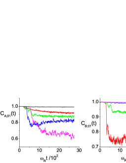
Figure 1: (Color online) Phase coherence of component A (on left) and component B (on right) for various populational fractions ($0\leq f_{B}<1$), for $N=5\times 10^{3}$, $\tau_{RU}=250/\omega_{R}$ = 11ms for ⁸⁷Rb. The numerical simulation shows the results from when lattice loading begins. The fractions of component B, $f_{B}$, and the line colors are (in the large $t$ limit, top to bottom on the left; bottom to top on the right): 0, black (for left side only); 0.1, red; 0.2, green; 0.4, blue; 0.6, pink.

Figure 1 shows the change in phase coherence between the center and nearest neighbor well, $C_{i;01}$, for component A (left) and B (right) from the time the lattice begins to ramp up, to a large time limit. The coherence changes for other distant wells ($C_{i;02},C_{i;03},C_{i;04}$, etc.) exhibit a similar pattern, but with more coherence loss at a given time. The first-order correlation functions between sites are closely related to the visibilities of the interference pattern Ramanan et al. (2009); Greiner et al. (2002). For one-component BEC cases, a complete loss of phase coherence would imply a transition to the Mott insulator state. In these calculations, the maximum lattice height does not reach the Mott insulator regime, as indicated by the observation that in Fig. 1, $C_{A;01}$ remains very close to unity if $f_{A}=1$. However, as $f_{B}$ increases, component A exhibits decoherence.

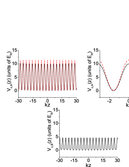
Figure 2: (Color online) The profile of combined potentials for the component A, $V_{c,A}(z)=V_{h,A}(z)+V_{o,A}(z)$ (black solid line on top left) and $V_{c,A}(z)=V_{h,A}(z)+V_{o,A}(z)+g_{AB}|\psi_{B}(z)|^{2}$ (red dashed line on top left) with $s_{max,A}=10$, and for the component B, $V_{c,B}(z)=V_{h,B}(z)+g_{AB}|\psi_{A}(z)|^{2}$ (on bottom). The figure on top right is the same plot on top left, but enlarged near the center of trap. The potentials, $V_{c,i}(z)$, are in units of $E_{R}$. The populations are $N_{A}=4\times 10^{3}$, $N_{B}=1\times 10^{3}$.

A new feature in this two-component case is the reduction of phase coherence of component B, which is induced as for component A but with the role of the optical lattice replaced by the atomic mean-field potential formed by component A’s periodic localization. In the GPE for the component B,

$$i\hbar\frac{\partial\psi_{B}(z,t)}{\partial t} = \big{[}L_{B}+g_{BB}|\psi_{B}(z,t)|^{2}$$ (28)

$$+g_{AB}|\psi_{A}(z,t)|^{2}\big{]}\psi_{B}(z,t),$$

such spatial variation of potential is expressed by the term $g_{AB}|\psi_{A}(x,t)|^{2}$. In Fig. 2, we show the optical lattice with the harmonic trap, which directly affects coherence properties of component A, and the mean-field lattice of A with the same harmonic trap, acting on component B, for the case $N=5\times 10^{3}$, $N_{A}=4\times 10^{3}$. The distortion by the harmonic trap potential is almost negligible around the center. We denote the atomic mean-field lattice made by component A as

$$I_{al,A}(z)=g_{AB}|\psi_{A}(z)|^{2}.$$ (29)

Then, the depth of the optical lattice and the interaction strength of the mean-field lattice are comparable ($(I_{al,A}(z)|_{max}-I_{al,A}(z)|_{min})/(V_{o,A}(z,t)|_{max}-V_{o,A}(z,t)|_{min})\simeq 0.6$) for $f_{B}/f_{A}=1/4$ as can be seen by Fig. 2.

Due to the presence of the mean-field lattice, the tunneling amplitude between the localization sites for component B is reduced, resulting in coherence loss, as shown on the right of Fig. 1.

The phase decoherence of component A is greater in the presence of component B than without component B, and increases as $f_{B}$ increases. Note also that the mean-field potential from B atoms acting on A atoms is in phase with the optical lattice, and thus effectively raises the periodic potential that A atoms see, therefore contributing to the loss of coherence of the A atoms. However, comparing with the degree of coherence for A atoms alone as a function of lattice height shown in the next section, elevation of the effective lattice acting on A atoms does not explain fully the decrease of coherence shown in Fig. 1 (left side). Evidently the stochastic nature of the atom distributions also plays a role.

The experiment in Gadway et al. (2010) has shown a similar dependency on populational fractions but with two peak-matched state-dependent optical lattices in order to place two components at the same lattice site.

To gain another perspective on these processes, we expand the wavefunctions in an array of Wannier-like orbitals, $w_{i}(z)$,

$$\hat{\psi}_{i}(z)=\sum_{l}\hat{a}_{il}w_{i}(z-R_{il}),$$ (30)

where the single particle wavefunction, $w_{i}(z-R_{il})$ is centered at $R_{Al}=(2l\pm 1)d/2$, $R_{Bl}=2ld/2$ for each component. We can approximate the Wannier functions as Gaussian functions and calculate on-site interaction energies and widths of on-site single-particle wavefunctions.

In Fig. 3, we show on-site interaction energies for component A and B as a function of the fraction of component B ($f_{B}$) using the same parameters as in the TWA simulations, $s_{max,A}=10$ and $N_{tot}=5\times 10^{3}$. Higher on-site energies, $U_{ii}$ correspond to greater localization, (smaller $\sigma_{i}$, where $\sigma_{i}$ is the width of the wavefunction in the $i$th well) and reduced nonlocal coherence, $C_{i,01}$.

Figure 3: The on-site interaction energies, $U_{ii}$ (solid line) and the widths of single-particle wavefunctions, $\sigma_{i}$ (dashed line) for component A (left) and for component B (right), showing opposite changes as the impurity component B populates increasingly. Here $s_{max,A}$=10, $N_{tot}=5\times 10^{3}$.

We now analyze phase coherence of component B. We begin with a bosonic mixture with a low population of component B, $f_{B}\simeq 0$, which can be approximated by the foreground component A with a B impurity. The average strength of interspecies interaction per B field ($\sim g_{AB}f_{A}N$) over its spatial variation, is greater when $f_{B}\simeq 0$ than when $f_{B}\simeq 1$. The interaction strength varies over space because of the component A’s modulational variance. This periodic mean field acts similarly to an optical lattice for component B, decreasing its phase coherence. On the other hand, the mixture with a high population of component B, $f_{B}\simeq 1$ ($q<1$), has weakened phase decoherence, which we can qualitatively interpret by the decreased strength of the mean-field lattice formed by the component A.

We now analyze phase coherence of component A. For a bosonic mixture with a low population of component B, $f_{B}\simeq 0$, the optical lattice alone does not substantially induce loss of phase coherence of component A. As $f_{B}$ increases, however, component A loses more phase coherence. The larger phase decoherence of component A as $f_{A}\rightarrow 0$ can be understood by the broadening of component B distribution enhanced by the narrowing of the A distribution. Due to the repulsive nature of interspecies interaction, the minimum energy is found in the balance between reducing the spatial overlap of the two-components’ amplitudes and weakening the intraspecies interaction energies of each component.

IV.2 A single lattice (A) with varying heights

In this section, we show how the phase coherence changes as a function of time, depending on the final lattice height for component A, in order to see the effect of mean-field lattice height. As in Sec. IV.1, $V_{o,B}(z,t)=0$, but now the atom numbers are fixed at $N_{A}=4.0\times 10^{3},N_{B}=1.0\times 10^{3}$. As before, the optical lattice for component A linearly increases up to the indicated value of $s_{max,A}$: the ramping-up time is $\omega_{R}\tau_{RU}=100$ in this case.

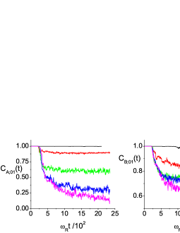
Figure 4: (Color online) The effect of final optical lattice heights on phase coherence of component A (on left) and component B (on right). The final lattice height ($s_{max,A}$) for each curve is following (top to bottom): the black line ($3$), the red line ($6.5$), the green line ($10$), the blue line ($13.5$), and the pink line ($17$).

Figure 5: The on-site interaction energies, $U_{ii}$ (solid line) and the widths of single-particle wavefunctions, $\sigma_{i}$ (dashed line) for component A ($U_{AA}$ on left) and for component B ($U_{BB}$ on right) for $N_{tot}=5\times 10^{3}$. Both components become more fragmented as the state-dependent optical lattice for only component A has been amplified more.

The changes in phase coherence, $C_{i;01}$, are shown in Fig. 4 for component A and B, and in Fig. 5, the on-site interaction energies are displayed for both components. As the lattice becomes deeper, the phase coherence of component A decreases as expected, since it is fragmented by the external lattice height increase even without consideration of interspecies effect. Decoherence of component B is enhanced as well because of the growth of the mean-field lattice from component A.

In light of interaction energies, an increase in the energy implies a smaller $\sigma$, similarly as seen in Fig. 3, hence tighter localization within the effective well. Thus Fig. 5 indicates, as expected, that the degree of localization is higher for deeper lattice heights. Comparing results between the two components in Fig. 5, the localization of component A is evidently stronger than component B for $s_{max,A}>10$, which explains the greater phase decoherence in component A than in component B in Fig. 4.

As is evident from comparing Figs. 5 and 3, when the A lattice height rises, the exchange of spatial occupation between the two components that has been observed in Sec. IV.1 does not occur. Component B’s localization is strengthened as well as component A’s. The loss in first-order spatial correlation between wells can be induced by increasing the height of barriers Spekkens and Sipe (1999), which for B atoms are provided by atomic mean-field lattices in this case.

IV.3 Two peak-mismatched lattices (A, B)

Up to this point, component B has not been subjected directly to an optical lattice, but is localized simply by interaction with the mean field resulting from component A, and the interspecies interaction. Additional insight into the localization process can come from applying to component B an optical lattice so as to strengthen the localization effect on B atoms on top of the former mean field. In other words, this section examines the dependence of phase decoherence of one component on the fragmentation of the other component in the presence of two peak-mismatch optical lattices as in Shi et al. (2008); Gubeskys and Malomed (2007). Intuitively, the addition of an optical lattice would additionally increase phase decoherence without limit. We will show in this section that it is not always the case.

To the BEC mixture with the asymmetric population ratio ($N_{A}=1.0\times 10^{3},N_{B}=4.0\times 10^{3}$), we gradually apply two state-dependent optical lattices:

$$V_{o,A}(z,t) = s_{A}(t)E_{R}\cos^{2}(kz),$$

$$V_{o,B}(z,t) = s_{B}(t)E_{R}\sin^{2}(kz),$$ (31)

where $s_{i}(t)=s_{max,i}t/\tau_{RU}$. The final lattice height for the component A is $s_{max,A}=10$ and the final lattice height for the component B is a variable parameter in different simulations ranging from $s_{max,B}=3$ to $s_{max,B}=17$ and all other conditions are the same as in the previous section.

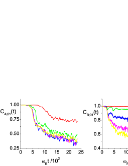
Figure 6: (Color online) The effect of localization induced by B on phase coherence on component A (on left) and component B (on right). The line colors and the final lattice heights for B ($s_{max,B}$) are following (explained below in parentheses for the left figure; top to bottom on the right): the red line, $3$ (top); the green line, $6.5$ (second to top); the blue line, $10$ (one of the two bottom curves); the pink line, $13.5$ (the other one of the two bottom curves); the yellow line, $17$ (between the bottom and the second to top).

Figure 7: The on-site interaction energies, $U_{ii}$ (solid line) and the widths of single-particle wavefunctions, $\sigma_{i}$ (dashed line) for component A ($U_{AA}$ on left) and for component B ($U_{BB}$ on right) as a function of the lattice height for B ($s_{max,B}$).

In Fig. 6, we show the change of phase coherence while varying the lattice height for component B. The drop in phase coherence of component B reflects the expectation that higher optical lattices induce more coherence loss between two neighboring sites. And also as expected, a higher lattice for component B leads to more localization for component B.

A new phenomenon here is the dependence of phase coherence of component A on optical lattice heights for the component B. As can be seen from Fig. 6 (left side), the phase coherence of component A at the maximum time shown is diminished as $s_{max,B}$ increases from 3 to 10, but then rises again for $s_{max,B}$ increases beyond 10. This non-monotonic dependence on the other component’s lattice height can also be seen in the on-site energy plotted in the left panel of Fig. 7, which shows a maximum of $U_{AA}$ at $s_{max,B}\sim 15$, and then a small decrease. In addition to the expected fragmentation due to the optical lattice applied directly to component A, the deepening mean-field potential from component B acting on component A further reduces the tunneling of component A between adjacent sites until the tunneling of component A suppressed by increased mean-field lattice height of component B becomes gradually freed by decreased wall width of the mean-field lattice ($\sigma_{B}$).

V Conclusion

In summary, we have investigated nonlocal intraspecies phase decoherence of two-component BECs under the gradual loading of state-dependent optical lattices. We have used the TWA and the Gaussian variational wavefunctions for Wannier orbitals to model the dynamical behavior and fragmentation of two species of atoms, in particular to calculate the reduction of phase coherence between wells.

First, when a single optical lattice acts on component A ($V_{o,A}\propto\cos^{2}(kz),V_{o,B}=0$), the B atoms are fragmented by the effective barriers produced by the interspecies repulsive interactions with A atoms. Thus, both species are fragmented into localized wells whose sites differ by a half-period between the two components. With varying fractions of a mixture, we have observed that when the fraction of B atoms increases, then in the long-time limit, the fragmentation of A atoms increases, but the fragmentation of B atoms decreases, consistent with experimental observations in Catani et al. (2008); Gadway et al. (2010). The increasing fragmentation of A atoms is associated with higher effective barriers produced by accumulation of B atoms spatially in phase with the A’s optical lattice. The decreasing fragmentation of B atoms is due to lower effective barriers produced by the reduced A mean-field lattice. With varying heights of the lattice, we have seen increasing fragmentation of both A and B atoms with higher lattice heights for A. We confirm that deep lattices for only a single component can play a key role for both components in reducing phase coherence.

Finally, when optical lattices are applied to both components with the condition that their well sites differ by a half-period ($V_{o,A}\propto\cos^{2}(kz),V_{o,B}\propto\sin^{2}(kz)$), then as the height of one of the lattices increases, phase decoherence of A atoms is limited and non-monotonic fragmentation occurs; the A atom on-site interaction energies reach a maximum, and then decrease while the other atoms (B) become more localized. This shows in a dramatic way how the effect of fragmentation (or equivalently, phase decoherence) of one species due to other component’s mean-field, can actually saturate.

All the calculations pertain to a situation in which the two species are different hyperfine states of the same atomic species, with equal masses and equal inter- and intra-species scattering lengths. Since this work is exploratory in nature, we have not attempted an extensive survey of parameter space by varying atom numbers, masses, and scattering lengths. We suggest that effects similar to what we obtain could occur if the two species were actually different types of atoms (Rb and K, for example), such as has been obtained in recent experiments.

Appendix A Initial states and TWA for two-component BECs

First, we generate a set of classical stochastic fields for the initial state sampled from the corresponding Wigner distribution function Gardiner (2004); Isella and Ruostekoski (2006) and obtain the dynamics of the system by averaging the statistical ensemble over individual trajectories in phase space. The expectation values of symmetrically-ordered operators are calculated from the weighted average of the corresponding classical fields ($\psi_{W}$) with the Wigner distribution function, $W(\psi_{W},\psi_{W}^{*})$ without extra modification terms.

The classical stochastic fields, $\alpha_{A0},\alpha_{B0},\alpha_{\mu}$ are obtained by randomly generating c-numbers that follow a given distribution, corresponding to quantum operators, $\hat{\alpha}_{A0},\hat{\alpha}_{B0}$, and $\hat{\alpha}_{\mu}$. Since the condensate mode operators and quasiparticle mode operators commute and the component A and B condensate operators also commute, we independently sample the c-numbers. For the condensate mode, the initial two-component superfluid state is approximated as a coexisting mixture of independent Glauber coherent states, where each coherent state preserves its own phase coherence. The Wigner function for the initial state is

$$W(\vec{\alpha},\vec{\alpha}^{*}) = W_{A0}(\alpha_{A0},\alpha_{A0}^{*})W_{B0}(\alpha_{B0},\alpha_{B0}^{*})$$ (32)

$$W_{BG}(\alpha,\alpha^{*}),$$

where $\vec{\alpha}=(\alpha_{A0},\alpha_{B0},\alpha_{\mu})^{T}$ and $W_{A0},W_{B0},W_{BG}$ are the Wigner distribution for the component A, the component B, and the Bogoliubov modes. The condensate mode Wigner distributions are given by ($i$ = A, B)

$$W_{i0}(\alpha_{i0},\alpha_{i0}^{*}) = \frac{2}{\pi}\exp{\big{[}-2|\alpha_{i0}-\sqrt{N_{i0}}|^{2}\big{]}},$$ (33)

where the ensemble averages are $\langle\alpha_{i0}\rangle_{W}=\sqrt{N_{i0}}$ and $\langle\alpha_{i0}^{*}\alpha_{i0}\rangle_{W}=N_{i0}+\frac{1}{2}$, and W denotes the ensemble average in the Wigner distribution. The distribution function of coherent states has a Gaussian profile in the complex phase space with a variance of $1/2$. For a large number of atoms ($N\gg 1$), quantum fluctuations around the mean classical field are relatively small, since $\Delta N/\langle N\rangle=1/\sqrt{\langle N\rangle}$. Thus we can think of the initial state as a classical field with a small fluctuation in phase space.

While the condensate modes have nonzero expectation values for the atom number of components, $\alpha_{i0}$, the noncondensate modes, $\alpha_{\mu}$ have zero expected populations, for which the Wigner distribution is the product of uncorrelated Wigner functions for each mode Blakie et al. (2008):

$$W_{BG}({\alpha,\alpha^{*}}) = \prod_{\mu}W_{\mu}(\alpha_{\mu},\alpha_{\mu}^{*}),$$

$$W_{\mu}(\alpha_{\mu},\alpha_{\mu}^{*}) = \frac{2}{\pi}\tanh{\Big{(}\frac{\epsilon_{\mu}}{k_{B}T}\Big{)}}$$ (34)

$$\exp{\bigg{[}-2|\alpha_{\mu}|^{2}\tanh{\Big{(}\frac{\epsilon_{\mu}}{k_{B}T}}\Big{)}\bigg{]}},$$

where $W_{BG}({\alpha,\alpha^{*}}),W_{\mu}(\alpha_{\mu},\alpha_{\mu}^{*})$ is the Wigner function for the total Bogoliubov modes and for each quasiparticle mode, respectively. The ensemble averages of quasiparticle modes satisfy the condition that they have zero mean values and Gaussian variances, which broaden as the temperature increases.

$$\langle\alpha_{\mu}\rangle_{W}=\langle\alpha_{\mu}^{*}\rangle_{W}=0,$$ (35)

$$\langle\alpha_{\mu}^{*}\alpha_{\nu}\rangle_{W}=\delta_{\mu\nu}[n_{\nu}+\frac{1}{2}].$$ (36)

Then, we construct a TWA method for the dynamics of two-component BECs under the nonequilibrium ramp-up of state-dependent optical lattices. We begin by projecting the above two-component state onto its phase space within the Wigner representation. We thereby obtain a quasi-probability distribution function over the phase space, which is formulated to be analogous to the density matrix in quantum mechanics Baker (1958); Steel et al. (1998). Even though a positive-P representation is sometimes used for simulations of a quantum system, it is subject to instabilities, for example in highly populated modes Steel et al. (1998). Instead, we approximate the dynamics of one-dimensional trapped multimode BECs by considering the Fokker-Planck equation in the truncated Wigner representation Steel et al. (1998).

The Fokker-Planck equation for the Wigner quasiprobability distribution yields the time evolution equation:

$$\frac{\partial W(\vec{\psi},\vec{\psi}^{*})}{\partial t}=\int dz\frac{i}{\hbar}\sum_{i,j=A,B}\bigg{[}\frac{\delta}{\delta\psi_{i}(z)}\Big{\{}L_{i}\hskip 28.45274pt\phantom{aaaa}$$

$$+g_{ij}(|\psi_{j}(z)|^{2}-d_{ij})\Big{\}}\psi_{i}(z)\phantom{aa}$$

$$-\frac{g_{ij}}{4}\frac{\delta}{\delta\psi_{i}(z)}\frac{\delta}{\delta\psi_{j}(z)}\frac{\delta}{\delta\psi_{j}^{*}(z)}\psi_{i}(z)\bigg{]}W(\vec{\psi},\vec{\psi}^{*})+h.c.,\phantom{aa}$$ (37)

where $\vec{\psi}=(\psi_{A},\psi_{B})^{T}$, and $d_{ij}=1\phantom{a}(\mathrm{or}\phantom{a}1/2)$ if $i=j\phantom{a}(\mathrm{or}\phantom{a}i\neq j)$.

The exact Fokker-Plank equation with the presence of the third-order term within the Wigner representation is difficult to solve both analytically and numerically in stochastic simulations Sinatra et al. (2002). Therefore, the truncation in the TWA neglects the third-order derivative terms in Eq. (37), which are smaller than the Gross-Pitaevskii first-order term in the total number, $N$. The second-order diffusion process term of usual stochastic processes, which can have a prominent role in enhancing fluctuations, is absent in the TWA. Also, in the TWA, the expectation values of those classical fields, $\prod_{i,j}\psi_{i}^{*}(z_{i})\psi_{j}(z_{j})$ in the Wigner representation, correspond to the expectation values of quantum operators that are symmetrically ordered. The Wigner quasiprobability distribution function, $W(\vec{\psi},\vec{\psi}^{*})$, is a classical projection function corresponding to the density operator for the field operators in quantum mechanics:

$$\langle\prod_{i,j}\hat{\psi}_{i}^{\dagger}(z_{i})\hat{\psi}_{j}(z_{j})\rangle_{W}=$$

$$\int d^{2}\vec{\psi}W(\vec{\psi},\vec{\psi}^{*})\prod_{i,j}\psi_{i}^{*}(z_{i})\psi_{j}(z_{j}).$$ (38)

Appendix B The Gaussian ansatz for Wannier functions

We expand the wavefunctions in an array of Wannier-like orbitals, $w_{i}(z)$,

$$\hat{\psi}_{i}(z)=\sum_{l}\hat{a}_{il}w_{i}(z-R_{il}),$$ (39)

where the single particle wavefunction, $w_{i}(z-R_{il})$ is centered at $R_{Al}=(2l\pm 1)d/2$, $R_{Bl}=2ld/2$ for each component, and the operators $\hat{a}_{il}$ satisfy the bosonic commutation relation, $[\hat{a}_{il},\hat{a}_{jl^{\prime}}^{\dagger}]=\delta_{ij}\delta_{ll^{\prime}}$. The variationally minimum solution of orbital wavefunctions implicitly depends on the occupation per site. Putting this set of orbitals into the Hamiltonian in Eq. (1), we obtain

$$H = -\sum_{i;ll^{\prime}}J_{i;ll^{\prime}}(\hat{a}_{il}^{\dagger}\hat{a}_{il^{\prime}}+\hat{a}_{il^{\prime}}^{\dagger}\hat{a}_{il})+\sum_{i;l}U_{ii}\hat{a}_{il}^{\dagger}\hat{a}_{il}^{\dagger}\hat{a}_{il}\hat{a}_{il}$$ (40)

$$+\sum_{l}U_{AB}\hat{a}_{Al}^{\dagger}\hat{a}_{Bl}^{\dagger}\hat{a}_{Al}\hat{a}_{Bl}+\sum_{i;l}\epsilon_{il}\hat{a}_{il}^{\dagger}\hat{a}_{il},$$

where

$$J_{i;ll^{\prime}} = -\int dzw_{i}(z-R_{il})$$

$$\bigg{[}-\frac{\hbar^{2}}{2m_{i}}\bigtriangledown^{2}+V_{h,i}(z)+V_{o,i}(z,t)\bigg{]}w_{i}(z-R_{il^{\prime}}),$$

$$U_{ij} = g_{ij}\int dzw_{i}^{2}(z-R_{il})w_{j}^{2}(z-R_{jl}).$$ (41)

In the tight-binding limit, the Wannier functions can be written as Gaussian functions Slater (1952). When the tight-binding limits $(V_{o,A}(z,t)|_{max}-V_{o,A}(z,t)|_{min})\gg E_{R}$ and $(I_{al,A}(z)|_{max}-I_{al,A}(z)|_{min})\gg E_{R}$ are achieved, the high vibrational modes for each component are not occupied especially at the initial temperature $T=0$ so that the profile of each component can be well described by the ground state, the Gaussian wavefunction. Starting from the initial trial state of infinite 1D BECs in the periodic state-dependent optical lattice, we employ the Gaussian variational ansatz for a single-particle orbital placed on each site, $w_{i}(z-R_{il})=(1/\pi\sigma_{i}^{2})^{1/4}\exp(-(z-R_{il})^{2}/2\sigma_{i}^{2})$, with the density of atoms per site equal to the average density of the center site calculated from the GPE ($n_{il}=n_{i0}^{(GPE)}$). Here, the widths of Gaussian wavefunctions are variational parameters, as in Pérez-García et al. (1997); Salasnich et al. (2002); Vignolo et al. (2003); Schaff et al. (2010).

Within the Gaussian approximation, we obtain the minimized Gross-Pitaevskii energy functional, where the interaction energies and the tunneling amplitudes can be calculated from variational parameters. The local single-band Gaussian state is known to be accurate for the calculation of on-site interaction energies even for shallow lattices ($\sim 3E_{R}$) with the overlap between the true Wannier function and the Gaussian wavefunction nearly equal to 1.0 Bloch et al. (2008). Since the Gaussian ansatz can be quite imprecise for the calculation of tunneling amplitudes because of the tail of Gaussian functions Bloch et al. (2008); Krämer et al. (2003), we concentrate on calculating on-site interaction energies.

Appendix C Numerical method

In this section, we explain the numerical methods implemented in this work. The condensation of cigar-shaped 1D atomic clouds is achieved in an anisotropic harmonic trap with the tight confinement along the transverse direction ($\omega_{z}=2\pi\times 130Hz,\omega_{\rho}=2\pi\times 2.71kHz$) and the aspect ratio is 21. In this work, the number of atoms ranges from $0.5\times 10^{3}$ to $5\times 10^{3}$. The optical lattices are generated by red-detuned off-resonant lasers with a wavelength $\lambda=785$ nm, so that the period is $d=\lambda/2=392.5$ nm, and the recoil frequency is $\omega_{R}=(\hbar/2m)(2\pi/\lambda)^{2}=2\pi\times 3.73$ kHz.

With $N_{tot}=5\times 10^{3}$, and the trap and lattice properties given above, we obtain as many as 75 atoms in the central well of the quasi-1D lattice. Experimentally, working also with ⁸⁷Rb, Campbell et al. Campbell et al. (2006) were able to put at most 5 atoms per site in their 3D optical lattice. Because of the tighter transverse confinement in Campbell et al. (2006), 75 atoms per well in our simulations would actually correspond to about 8 atoms per well in Campbell et al. (2006) for the same density at the peak. In actual experiments, the total number of atoms would need to be reduced over the value used here. This would lead to a reduction of the demonstrated coherence loss effects.

The one-dimensionality of cigar-shaped BECs in the harmonic trap at $T=0$ is achieved when $l_{z}>\xi>l_{\rho}$ or $\mu_{3D}<\hbar\omega_{\rho}$ Görlitz et al. (2001), where $l_{z}=(\hbar/m\omega_{z})^{1/2}$ and $l_{\rho}=(\hbar/m\omega_{\rho})^{1/2}$ are the longitudinal and the transverse zero-point oscillation length respectively, $\xi=(1/4\pi n_{3D}a_{s})^{1/2}$ is the healing length, and $\mu_{3D}=\hbar^{2}/2m(15Na_{s}/l_{z}^{2}l_{\rho}^{4})$ is the chemical potential corresponding to the interaction energy. Furthermore at $T>0$, $l_{\rho}$ is required to be smaller than the de Broglie wavelength $\lambda_{T}$ ($l_{\rho}<\lambda_{T}$), where $\lambda_{T}=(2\pi\hbar^{2}/mT)^{1/2}$ Kheruntsyan et al. (2003). For the ⁸⁷Rb atoms in a trap with frequencies given above, the ratios, $l_{\rho}/\xi\lesssim 2$ and $\mu_{3D}/\hbar\omega_{\rho}\lesssim 3$.

Each BEC component lies in the Thomas-Fermi regime between the full 3D dynamics and the true 1D dynamics with transverse excitations almost frozen out. Even though the BEC is in the crossover between 3D and 1D, the low-energy excitation modes in 3D are effectively 1D provided that the temperature is sufficiently below the energy of the transverse oscillator ($T<\hbar\omega_{\rho}$) Stringari (1998) which is the case here ($T=0$). The Thomas-Fermi radius ranges from $5$ to $12l_{z}$.

The dimensionless coupling strength of interaction energies in this work is $\gamma=mg_{1D}/\hbar^{2}n_{1D}\lesssim 2\times 10^{-3}$ and the reduced temperature is $\tau=2mk_{B}T/\hbar^{2}n_{1D}^{2}=0$ Gangardt and Shlyapnikov (2003). Therefore, the 1D Bose gas can be effectively described by the Gross-Pitaevskii equation in the regime ($\tau^{2}\lesssim\gamma\lesssim 1$) far from the Tonks-Girardeau regime ($\gamma\gtrsim 1$). The nonlinearity $g_{1D}N/\hbar\omega_{z}l_{z}$ Isella and Ruostekoski (2006) ranges from $120$ to $1200$.

The numerical preparation of initial states requires ground state wavefunctions, the Bogoliubov quasiparticle excited modes, and their stochastic distributions governed by the Wigner functions. We find the ground state wavefunctions by numerically integrating the GPE in imaginary time with a time step of $\omega_{R}\delta t=0.005$ with 3072 spatial grid points along the axial direction. We utilize the second-order split-operator method to integrate the time evolution of wavefunctions, in nonlinear as well as linear regimes. Using the ground state solutions of the GPE, we obtain quasiparticle wavefunctions, $u_{A\mu}(z),u_{B\mu}(z),v_{A\mu}(z),v_{B\mu}(z)$ for energy, $\epsilon_{\mu}$ by the diagonalization of the Bogoliubov-de Gennes equation [Eq. 23].

We calculate the ensemble average of stochastic fields along the trajectory and find their coherence. Stochastic quantum fluctuations are appended to the initial mean-field state for generation of the ensemble of Wigner-distributed initial states, in which step we perform the Gaussian random variable generation of order parameters ($\alpha_{i0},\alpha_{\mu}$). For the condensate mode, the mean of $\alpha_{i0}$ is $\sqrt{N_{i0}}$ and its width of deviation is $\sqrt{1/2}$, whereas for the Bogoliubov quasiparticle mode, the mean of $\alpha_{\mu}$ is zero and the width is $\sqrt{1/2}$ for $T=0$. A single sample of stochastic fields, $\psi_{W}(x)$ is obtained by configuring the wavefunction profiles with the generated stochastic order parameters.

The condition for numerical validity of the TWA method in the Bogoliubov theory is that the condensate mode must be highly populated compared to the noncondensate mode so that the quantum fluctuation is small, being dominated by the condensate field. In other words, the TWA in the mean-field theory is valid with a relatively small number of excited Bogoliubov quasi-particles compared to the number of condensate particles in the system, $N\gg M/2$, where N is the total number of atoms, M is the number of Bogoliubov quasi-particles. This is a regime different from other exact numerical methods, for example, the Time Evolving Block Decimation (TEBD) method or the Density Matrix Renormalization Group (DMRG) with the Bose-Hubbard Model, in which cases each site is limited to a low filling factor since the Hilbert space increases exponentially with the number of atoms and the number of sites.

We perform the simulation with an ensemble of states consisting of 500 samples for the TWA distribution function to achieve sufficient convergence. The time evolution of ensembles has the typical time step given by $\omega_{R}\delta t=0.005$, i.e. $\delta t$ = 0.2 $\mu$s.

References

- Jaksch and Zoller (2005) D. Jaksch and P. Zoller, Annals of Physics 315, 52 (2005).
- Lewenstein et al. (2007) M. Lewenstein, A. Sanpera, V. Ahufinger, Bogdan Damski, A. Sen, and U. Sen, Advances in Physics 56, 243 (2007).
- Fisher et al. (1989) M. P. A. Fisher, P. B. Weichman, G. Grinstein, and D. S. Fisher, Physical Review B 40, 546 (1989).
- Jaksch et al. (1998) D. Jaksch, C. Bruder, J. I. Cirac, C. W. Gardiner, and P. Zoller, Physical Review Letters 81, 3108 (1998).
- Greiner et al. (2002) M. Greiner, O. Mandel, T. Esslinger, T. W. Hänsch, and I. Bloch, Nature 415, 39 (2002).
- Stöferle et al. (2004) T. Stöferle, H. Moritz, C. Schori, Michael Köhl, and T. Esslinger, Physical Review Letters 92, 130403 (2004).
- Orzel et al. (2001) C. Orzel, A. K. Tuchman, M. L. Fenselau, M. Yasuda, and M. A. Kasevich, Science 291, 2386 (2001).
- Polak and Kopeć (2010) T. P. Polak and T. K. Kopeć, Physical Review A 81, 043612 (2010).
- Buonsante et al. (2008) P. Buonsante, S. M. Giampaolo, F. Illuminati, V. Penna, and A. Vezzani, Physical Review Letters 100, 240402 (2008).
- Polak and Kopec (2008) T. P. Polak and T. K. Kopec, Annalen Der Physik 17, 947 (2008).
- Thalhammer et al. (2008) G. Thalhammer, G. Barontini, L. De Sarlo, J. Catani, F. Minardi, and M. Inguscio, Physical Review Letters 100, 210402 (2008).
- Catani et al. (2009) J. Catani, G. Barontini, G. Lamporesi, F. Rabatti, G. Thalhammer, F. Minardi, S. Stringari, and M. Inguscio, Physical Review Letters 103, 140401 (2009).
- Pertot et al. (2010) D. Pertot, B. Gadway, and D. Schneble, Physical Review Letters 104, 200402 (2010).
- Hamner et al. (2011) C. Hamner, J. J. Chang, P. Engels, and M. A. Hoefer, Physical Review Letters 106, 065302 (2011).
- Soltan-Panahi et al. (2011) P. Soltan-Panahi, J. Struck, P. Hauke, A. Bick, W. Plenkers, G. Meineke, C. Becker, P. Windpassinger, M. Lewenstein, and K. Sengstock, Nat Phys 7, 434 (2011).
- Catani et al. (2008) J. Catani, L. De Sarlo, G. Barontini, F. Minardi, and M. Inguscio, Physical Review A 77, 011603 (2008).
- Gadway et al. (2010) B. Gadway, D. Pertot, R. Reimann, and D. Schneble, Physical Review Letters 105, 045303 (2010).
- Altman et al. (2003) E. Altman, W. Hofstetter, E. Demler, and M. D. Lukin, New Journal of Physics 5, 113 (2003).
- Isacsson et al. (2005) A. Isacsson, M. C. Cha, K. Sengupta, and S. M. Girvin, Physical Review B 72, 184507 (2005).
- Krutitsky and Graham (2003) K. V. Krutitsky and R. Graham, Physical Review Letters 91, 240406 (2003).
- Larson and Martikainen (2008) J. Larson and J. P. Martikainen, Physical Review A 78, 063618 (2008).
- Ruostekoski and Dutton (2007) J. Ruostekoski and Z. Dutton, Physical Review A 76, 063607 (2007).
- Wernsdorfer et al. (2010) J. Wernsdorfer, M. Snoek, and W. Hofstetter, Physical Review A 81, 043620 (2010).
- Cipolatti et al. (2016) R. Cipolatti, L. Villegas-Lelovsky, M. C. Chung, and C. Trallero-Giner, Journal of Physics A: Mathematical and Theoretical 49, 145201 (2016).
- Guglielmino et al. (2010) M. Guglielmino, V. Penna, and B. Capogrosso-Sansone, Physical Review A 82, 021601 (2010).
- Li et al. (2013) Y. Li, L. He, and W. Hofstetter, New Journal of Physics 15, 093028 (2013).
- Hofer et al. (2012) P. P. Hofer, C. Bruder, and V. M. Stojanović, Physical Review A 86, 033627 (2012).
- Shrestha and Ruostekoski (2012) U. Shrestha and J. Ruostekoski, New Journal of Physics 14, 043037 (2012).
- Xi et al. (2014) K.-T. Xi, J. Li, and D.-N. Shi, Physica B: Condensed Matter 436, 149 (2014).
- Cockburn et al. (2011) S. P. Cockburn, A. Negretti, N. P. Proukakis, and C. Henkel, Physical Review A 83, 043619 (2011).
- Isella and Ruostekoski (2006) L. Isella and J. Ruostekoski, Physical Review A 74, 063625 (2006).
- Bruderer et al. (2007) M. Bruderer, A. Klein, S. R. Clark, and Dieter Jaksch, Physical Review A 76, 011605 (2007).
- Hu et al. (2009) A. Hu, L. Mathey, I. Danshita, E. Tiesinga, C. J. Williams, and C. W. Clark, Physical Review A 80, 023619 (2009).
- Zaleski and Kopeć (2011) T. A. Zaleski and T. K. Kopeć, Physical Review A 84, 053613 (2011).
- Zheng and Gu (2013) H.-L. Zheng and Q. Gu, Frontiers of Physics 8, 375 (2013).
- Sajna et al. (2015) A. S. Sajna, T. P. Polak, R. Micnas, and P. Rożek, Physical Review A 92, 013602 (2015).
- Yanay and Mueller (2016) Y. Yanay and E. J. Mueller, Physical Review A 93, 013622 (2016).
- McKagan et al. (2006) S. B. McKagan, D. L. Feder, and W. P. Reinhardt, Physical Review A 74, 013612 (2006).
- Gardiner (1992) C. W. Gardiner, Quantum Noise (Springer-Verlag, 1992).
- Walls and Milburn (2008) D. F. Walls and G. J. Milburn, Quantum Optics (Springer, 2008).
- Bistritzer and Altman (2007) R. Bistritzer and E. Altman, Proceedings of the National Academy of Sciences 104, 9955 (2007).
- Gardiner (2004) C. W. Gardiner, Handbook of Stochastic Methods: For Physics, Chemistry and the Natural Sciences, 3rd ed. (Springer, 2004).
- Hall et al. (1998) D. S. Hall, M. R. Matthews, J. R. Ensher, C. E. Wieman, and E. A. Cornell, Physical Review Letters 81, 1539 (1998).
- Ozeri et al. (2005) R. Ozeri, N. Katz, J. Steinhauer, and N. Davidson, Reviews of Modern Physics 77, 187 (2005).
- Blakie et al. (2008) P. B. Blakie, A. S. Bradley, M. J. Davis, R. J. Ballagh, and C. W. Gardiner, Advances in Physics 57, 363 (2008).
- Sinatra et al. (2002) A. Sinatra, C. Lobo, and Y. Castin, Journal of Physics B: Atomic, Molecular and Optical Physics 35, 3599 (2002).
- Sinatra et al. (2001) A. Sinatra, C. Lobo, and Y. Castin, Physical Review Letters 87, 210404 (2001).
- Gardiner (1997) C. W. Gardiner, Physical Review A 56, 1414 (1997).
- Castin and Dum (1997) Y. Castin and R. Dum, Physical Review Letters 79, 3553 (1997).
- Castin and Dum (1998) Y. Castin and R. Dum, Physical Review A 57, 3008 (1998).
- Steel et al. (1998) M. J. Steel, M. K. Olsen, L. I. Plimak, P. D. Drummond, S. M. Tan, M. J. Collett, D. F. Walls, and R. Graham, Physical Review A 58, 4824 (1998).
- Ramanan et al. (2009) S. Ramanan, T. Mishra, M. S. Luthra, R. V. Pai, and B. P. Das, Physical Review A 79, 013625 (2009).
- Spekkens and Sipe (1999) R. W. Spekkens and J. E. Sipe, Physical Review A 59, 3868 (1999).
- Shi et al. (2008) Z. Shi, K. J. H. Law, P. G. Kevrekidis, and B. A. Malomed, Physics Letters A 372, 4021 (2008).
- Gubeskys and Malomed (2007) A. Gubeskys and B. A. Malomed, Physical Review A 75, 063602 (2007).
- Baker (1958) G. A. Baker, Physical Review 109, 2198 (1958).
- Slater (1952) J. C. Slater, Physical Review 87, 807 (1952).
- Pérez-García et al. (1997) V. M. Pérez-García, H. Michinel, J. I. Cirac, M. Lewenstein, and P. Zoller, Physical Review A 56, 1424 (1997).
- Salasnich et al. (2002) L. Salasnich, A. Parola, and L. Reatto, Physical Review A 65, 043614 (2002).
- Vignolo et al. (2003) P. Vignolo, Z. Akdeniz, and M. P. Tosi, Journal of Physics B: Atomic, Molecular and Optical Physics 36, 4535 (2003).
- Schaff et al. (2010) J. F. Schaff, Z. Akdeniz, and P. Vignolo, Physical Review A 81, 041604 (2010).
- Bloch et al. (2008) I. Bloch, J. Dalibard, and W. Zwerger, Reviews of Modern Physics 80, 885 (2008).
- Krämer et al. (2003) M. Krämer, C. Menotti, L. Pitaevskii, and S. Stringari, The European Physical Journal D 27, 247 (2003).
- Campbell et al. (2006) G. K. Campbell, J. Mun, M. Boyd, P. Medley, A. E. Leanhardt, L. G. Marcassa, D. E. Pritchard, and W. Ketterle, Science 313, 649 (2006).
- Görlitz et al. (2001) A. Görlitz, J. M. Vogels, A. E. Leanhardt, C. Raman, T. L. Gustavson, J. R. Abo-Shaeer, A. P. Chikkatur, S. Gupta, S. Inouye, T. Rosenband, and W. Ketterle, Physical Review Letters 87, 130402 (2001).
- Kheruntsyan et al. (2003) K. V. Kheruntsyan, D. M. Gangardt, P. D. Drummond, and G. V. Shlyapnikov, Physical Review Letters 91, 040403 (2003).
- Stringari (1998) S. Stringari, Physical Review A 58, 2385 (1998).
- Gangardt and Shlyapnikov (2003) D. M. Gangardt and G. V. Shlyapnikov, Physical Review Letters 90, 010401 (2003).