Asynchronous Partial Overlay: A New Algorithm for Solving Distributed Constraint Satisfaction Problems

\nameRoger Mailler \emailmailler@ai.sri.com
\addrSRI International
333 Ravenswood Dr
Menlo Park, CA 94025 USA \AND\nameVictor R. Lesser \emaillesser@cs.umass.edu
\addrUniversity of Massachusetts, Department of Computer Science
140 Governors Drive
Amherst, MA 01003 USA

Abstract

Distributed Constraint Satisfaction (DCSP) has long been considered an important problem in multi-agent systems research. This is because many real-world problems can be represented as constraint satisfaction and these problems often present themselves in a distributed form. In this article, we present a new complete, distributed algorithm called asynchronous partial overlay (APO) for solving DCSPs that is based on a cooperative mediation process. The primary ideas behind this algorithm are that agents, when acting as a mediator, centralize small, relevant portions of the DCSP, that these centralized subproblems overlap, and that agents increase the size of their subproblems along critical paths within the DCSP as the problem solving unfolds. We present empirical evidence that shows that APO outperforms other known, complete DCSP techniques.

1 Introduction

The Distributed constraint satisfaction problem has become a very useful representation that is used to describe a number of problems in multi-agent systems including distributed resource allocation (?) and distributed scheduling (?). Some researchers in cooperative multi-agent systems have focused on developing methods for solving these problems that are based on one key assumption. Particularly, the agents involved in the problem solving process are autonomous. This means that the agents are only willing to exchange information that is directly relevant to the shared problem and retain the ability to refuse a solution when it obviously conflicts with some internal goal.

These researchers believe that the focus on agent autonomy precludes the use of centralization because it forces the agents to reveal all of their internal constraints and goals which may, for reasons of privacy or pure computational complexity, be impossible to achieve. Several algorithms have been developed with the explicit purpose of allowing the agents to retain their autonomy even when they are involved in a shared problem which exhibits interdependencies. Probably the best known algorithms that fit this description can be found in the work of Yokoo et al. in the form of distributed breakout (DBA) (?), asynchronous backtracking (ABT) (?), and asynchronous weak-commitment (AWC) (?).

Unfortunately, a common drawback to each of these algorithms is that in an effort to provide the agents which complete privacy, these algorithms prevent the agents from making informed decisions about the global effects of changing their local allocation, schedule, value, etc. For example, in AWC, agents have to try a value and wait for another agent to tell them that it will not work through a $nogood$ message. Because of this, agents never learn true reason why another agent or set of agents is unable to accept the value, they only learn that their value in combination with other values doesn’t work.

In addition, these techniques suffer because they have complete distribution of the control. In other words, each agent makes decisions based on its incomplete and often inaccurate view of the world. The result is that this leads to unnecessary thrashing in the problem solving because the agents are trying to adapt to the behavior of the other agents, who in turn are trying to adapt to them. Pathologically, this behavior can be counter-productive to convergence of the protocol(?).

This iterative trial and error approach to discovering the implicit and implied constraints within the problem causes the agents to pass an exponential number of messages and actually reveals a great deal of information about the agents’ constraints and domain values (?). In fact, in order to be complete, agents using AWC have to be willing to reveal all of their shared constraints and domain values. The key thing to note about this statement is that AWC still allows the agents to retain their autonomy even if they are forced to reveal information about the variables and constraints that form the global constraint network.

In this paper, we present a cooperative mediation based DCSP protocol, called Asynchronous Partial Overlay (APO). Cooperative mediation represents a new methodology that lies somewhere between centralized and distributed problem solving because it uses dynamically constructed, partial centralization. This allows cooperative mediation based algorithms, like APO, to utilize the speed of current state-of-the-art centralized solvers while taking advantage of opportunities for parallelism by dynamically identifying relevant problem structure.

APO works by having agents asynchronously take the role of mediator. When an agent acts as a mediator, it computes a solution to a portion of the overall problem and recommends value changes to the agents involved in the mediation session. If, as a result of its recommendations, it causes conflicts for agents outside of the session, it links with them preventing itself from repeating the mistake in future sessions.

Like AWC, APO provides the agents with a great deal of autonomy by allowing anyone of them to take over as the mediator when they notice an undesirable state in the current solution to the shared problem. Further adding to their autonomy, agents can also ignore recommendations for changing their local solution made by other agents. In a similar way to AWC, APO is both sound and complete when the agents are willing to reveal the domains and constraints of their shared variables and allows the agents to obscure the states, domains, and constraints of their strictly local variables.

In the rest of this article, we present a formalization of the DCSP problem (section 2). In section 3, we describe the underlying assumptions and motivation for this work. We then present the APO algorithm (section 4.1) and give an example of the protocol’s execution on a simple 3-coloring problem (section 4.2). We go on to give the proofs for the soundness and completeness of the algorithm (section 4.3). In section 5, we present the results of extensive testing that compares APO with AWC within the distributed graph coloring domain and the complete compatibility version of the SensorDCSP domain (?) across a variety of metrics including number of cycles, messages, bytes transmitted, and serial runtime. In each of these cases, we will show that APO significantly outperforms AWC (?, ?). Section 6 summarizes the article and discusses some future research directions.

2 Distributed Constraint Satisfaction

A Constraint Satisfaction Problem (CSP) consists of the following:

•

a set of n variables $V=\{x_{1},\ldots,x_{n}\}$ .
•

discrete, finite domains for each of the variables $D=\{D_{1},\ldots,D_{n}\}$ .
•

a set of constraints $R=\{R_{1},\ldots,R_{m}\}$ where each $R_{i}(d_{i1},\ldots,d_{ij})$ is a predicate on the Cartesian product $D_{i1}\times\cdots\times D_{ij}$ that returns true iff the value assignments of the variables satisfies the constraint.

The problem is to find an assignment $A=\{d_{1},\ldots,d_{n}|d_{i}\in D_{i}\}$ such that each of the constraints in $R$ is satisfied. CSP has been shown to be NP-complete, making some form of search a necessity.

In the distributed case, DCSP, using variable-based decomposition, each agent is assigned one or more variables along with the constraints on their variables. The goal of each agent, from a local perspective, is to ensure that each of the constraints on its variables is satisfied. Clearly, each agent’s goal is not independent of the goals of the other agents in the system. In fact, in all but the simplest cases, the goals of the agents are strongly interrelated. For example, in order for one agent to satisfy its local constraints, another agent, potentially not directly related through a constraint, may have to change the value of its variable.

In this article, for the sake of clarity, we restrict ourselves to the case where each agent is assigned a single variable and is given knowledge of the constraints on that variable. Since each agent is assigned a single variable, we will refer to the agent by the name of the variable it manages. Also, we restrict ourselves to considering only binary constraints which are of the form $R_{i}(d_{i1},d_{i2})$ . Since APO uses centralization as its core, it is easy to see that the algorithm would work if both of these restrictions are removed. This point will be discussed as part of the algorithm description in section 4.1.4.

Throughout this article, we use the term constraint graph to refer to the graph formed by representing the variables as nodes and the constraints as edges. Also, a variable’s neighbors are the variables with which it shares constraints.

3 Assumptions and Motivation

3.1 Assumptions

The following are the assumptions made about the environments and agents for which this protocol was designed:

1.

Agents are situated, autonomous, computing entities. As such, they are capable of sensing their environment, making local decisions based on some model of intentionality, and acting out their decisions. Agents are rationally and resource bounded. As a result, agents must communicate to gain information about each others state, intentions, decisions, etc.
2.

Agents within the multi-agent system share one or more joint goals. In this paper, this goal is Boolean in nature stemming from the DCSP formulation.
3.

Because this work focuses on cooperative problem solving, the agents are cooperative. This does not necessarily imply they will share all of their state, intentions, etc. with other agents, but are, to some degree, willing to exchange information to solve joint goals. It also does not imply that they will change their intentions, state, or decisions based on the demands of another agent. Agents still maintain their autonomy and the ability to refuse or revise the decisions of other agents based on their local state, intentions, decisions, etc.
4.

Each agent has the capability of computing solutions to the joint goal based on their potentially limited rationality. This follows naturally from the ability of agents to make their own decisions, i.e., every agent is capable of computing a solution to its own portion of the joint goal based on its own desires.

3.2 Motivation for Mediation-Based Problem Solving

The Websters dictionary defines the act of mediating as follows:

Mediate: 1. to act as an intermediary; especially to work with opposing sides in order to resolve (as a dispute) or bring about (as a settlement). 2. to bring about, influence, or transmit by acting as an intermediate or controlling agent or mechanism. (?)

By its very definition, mediation implies some degree of centralizing a shared problem in order for a group of individuals to derive a conflict free solution. Clearly in situations where the participants are willing (cooperative), mediation is a powerful paradigm for solving disputes. It’s rather strange, considering this, that very little has been done on looking at mediation as a cooperative method for solving DCSPs.

Probably, the earliest mediation-based approach for solving conflicts amongst agents in an airspace management application(?). This work investigates using various conflict resolution strategies to deconflict airspace in a distributed air traffic control system. The author proposes a method for solving disputes where the involved agents elect a leader to solve the problem. Once elected, the leader becomes responsible for recognizing the dispute, devising a plan to correct it, and acting out the plan. Various election schemes are tested, but unfortunately, the leader only has authority to modify its own actions in order to resolve the conflicts. This obviously leads to situations where the plan is suboptimal.

In (?), the authors describe mediation as one of a number possible coordination mechanisms. In this work, the mediator acts as a intermediary between agents and can also act to coordinate their behavior. As an intermediary, the mediator routes messages, provides directory services, etc. This provides for a loose coupling of the agents, since they only need to know the mediator. The mediator can also act to coordinate the agents behavior if they have tight interdependencies.

Most of the research work on mediation-based problem solving involved settling disputes between competitive or semi-competitive agents. Probably one of the best examples of using mediation in this manner can be found in the PERSUADER system(?). PERSUADER was designed to settle conflicts between adversarial parties that are involved in a labor dispute. PERSUADER uses case-based reasoning to suggest concessions in order to converge on a satisfactory solution. Another example of using mediation in this way can be found in in a system called Designer Fabricator Interpreter (DFI) (?). In DFI, mediation is used to resolve conflicts as one of a series of problem solving steps. Whenever the first step fails, in this case iterative negotiation, a mediator agent steps in and tries to convince the agents to relax their constraints. If this fails, the mediator mandates a final solution.

There may be several reasons why mediation has not been more deeply explored as a cooperative problem solving method. First, researchers have focused strongly on using distributed computing as a way of exploiting concurrency to distribute the computation needed to solve hard problems (?). Because of this, even partially and/or temporarily centralizing sections of the problem can be viewed as contradictory to the central goal. Second, researchers have often claimed that part of the power of the distributed methods lies in the ability of the techniques to solve problems that are naturally distributed. For example, supply chain problems generally have no central monitoring authority. Again, directly sharing the reasons why a particular choice is made in the form of a constraint can seem to contradict the use of distributed methods. Lastly, researchers often claim that for reasons of privacy or security the problem should be solved in a distributed fashion. Clearly, sharing information to solve a problem compromises an agents ability to be private and/or violates its security in some manner.

Refer to caption — Figure 1: A simple distributed problem with two variables.

Although, parallelism, natural distribution, security, and privacy, may all seem like good justifications for entirely distributed problem solving, in actuality, whenever a problem has interdependencies between distributed problem solvers, some degree of centralization and information sharing must take place in order to derive a conflict-free solution.

Consider, as a simple example, the problem in figure 1. In this figure, two problem solvers, each with one variable, share the common goal of having a different value from one another. Each of the agents has only two allowable values: {1, 2}. Now, in order to solve this problem, each agent must individually decide that they have a different value from the other agent. To do this, at the very least, one agent must transmit its value to the other. By doing this, it removes half of its privacy (by revealing one of its possible values), eliminates security (because the other agent could make him send other values by telling him that this value is no good), and partially centralizes the problem solving (agent S2 has to compute solutions based on the solution S1 presented and decide if the problem is solved and agent S1 just relies on S2 to solve it.) In even this simple example, achieving totally distributed problem solving is impossible.

In fact, if you look at the details of any of the current approaches to solving DCSPs, you will observe a significant amount of centralization occurring. Most of these approaches perform this centralization incrementally as the problem solving unfolds in an attempt to restrict the amount of internal information being shared. Unfortunately, on problems that have interdependencies among the problem solvers, revealing an agent’s information (such as the potential values of their variables) is unavoidable. In fact, solutions that are derived when one or more agents conceals all of the information regarding a shared constraint or variable are based on incomplete information and therefore may not always be sound.

It follows then, that since you cannot avoid some amount of centralization, mediation is a natural method for solving problems that contain interdependencies among distributed problem solvers.

4 Asynchronous Partial Overlay

As a cooperative mediation based protocol, the key ideas behind the creation of the APO algorithm are

•

Using mediation, agents can solve subproblems of the DCSP using internal search.
•

These local subproblems can and should overlap to allow for more rapid convergence of the problem solving.
•

Agents should, over time, increase the size of the subproblem they work on along critical paths within the CSP. This increases the overlap with other agents and ensures the completeness of the search.

4.1 The Algorithm

Figures 2, 3, 4, 5, and 6 present the basic APO algorithm. The algorithm works by constructing a $good\_list$ and maintaining a structure called the $agent\_view$ . The $agent\_view$ holds the names, values, domains, and constraints of variables to which an agent is linked. The $good\_list$ holds the names of the variables that are known to be connected to the owner by a path in the constraint graph.

As the problem solving unfolds, each agent tries to solve the subproblem it has centralized within its $good\_list$ or determine that it is unsolvable which indicates the entire global problem is over-constrained. To do this, agents take the role of the mediator and attempt to change the values of the variables within the mediation session to achieve a satisfied subsystem. When this cannot be achieved without causing a violation for agents outside of the session, the mediator links with those agents assuming that they are somehow related to the mediator’s variable. This process continues until one of the agents finds an unsatisfiable subsystem, or all of the conflicts have been removed.

In order to facilitate the problem solving process, each agent has a dynamic priority that is based on the size of their $good\_list$ (if two agents have the same sized $good\_list$ then the tie is broken using the lexicographical ordering of their names). Priorities are used by the agents to decide who mediates a session when a conflicts arises. Priority ordering is important for two reasons. First, priorities ensure that the agent with the most knowledge gets to make the decisions. This improves the efficiency of the algorithm by decreasing the effects of myopic decision making. Second, priorities improve the effectiveness of the mediation process because lower priority agents expect higher priority agents to mediate. This improves the likelihood that lower priority agents will be available when a mediation request is sent.

procedure initialize $d_{i}\leftarrow random\ d\in D_{i}$ ; $p_{i}\leftarrow sizeof(neighbors)+1$ ; $m_{i}\leftarrow$ true; $mediate\leftarrow$ false; add $x_{i}$ to the $good\_list$ ; send (init, ( $x_{i},p_{i},d_{i},m_{i},D_{i},C_{i}$ )) to neighbors; $initList\leftarrow$ neighbors; end initialize; when received (init, ( $x_{j},p_{j},d_{j},m_{j},D_{j},C_{j}$ )) do Add ( $x_{j},p_{j},d_{j},m_{j},D_{j},C_{j}$ ) to agent_view; if $x_{j}$ is a neighbor of some $x_{k}\in good\_list$ do add $x_{j}$ to the good_list; add all $x_{l}\in agent\_view\land x_{l}\notin good\_list$ that can now be connected to the good_list; $p_{i}\leftarrow sizeof(good\_list)$ ; end if; if $x_{j}\notin initList$ do send (init, ( $x_{i},p_{i},d_{i},m_{i},D_{i},C_{i}$ )) to $x_{j}$ ; else remove $x_{j}$ from initList; check_agent_view; end do;

Figure 2: The APO procedures for initialization and linking.

4.1.1 Initialization (Figure 2)

On startup, the agents are provided with the value (they pick it randomly if one isn’t assigned) and the constraints on their variable. Initialization proceeds by having each of the agents send out an “init” message to its neighbors. This initialization message includes the variable’s name ( $x_{i}$ ), priority ( $p_{i}$ ), current value( $d_{i}$ ), the agent’s desire to mediate ( $m_{i}$ ), domain ( $D_{i}$ ), and constraints ( $C_{i}$ ). The array initList records the names of the agents that initialization messages have been sent to, the reason for which will become immediately apparent.

when received (ok?, ( $x_{j},p_{j},d_{j},m_{j}$ )) do update agent_view with $(x_{j},p_{j},d_{j},m_{j})$ ; check_agent_view; end do; procedure check_agent_view if $initList\neq\emptyset$ or $mediate\neq$ false do return; $m^{\prime}_{i}\leftarrow hasConflict(x_{i})$ ; if $m^{\prime}_{i}$ and $\neg\exists_{j}(p_{j}>p_{i}\land m_{j}=\,={\bf true})$ if $\exists(d^{\prime}_{i}\in D_{i})\ (d^{\prime}_{i}\cup agent\_view$ does not conflict) and $d_{i}$ conflicts exclusively with lower priority neighbors $d_{i}\leftarrow d^{\prime}_{i}$ ; send (ok?, ( $x_{i},p_{i},d_{i},m_{i}$ )) to all $x_{j}\in agent\_view$ ; else do mediate; else if $m_{i}\neq m^{\prime}_{i}$ $m_{i}\leftarrow m^{\prime}_{i}$ ; send (ok?, ( $x_{i},p_{i},d_{i},m_{i}$ )) to all $x_{j}\in agent\_view$ ; end if; end check_agent_view;

Figure 3: The procedures for doing local resolution, updating the agent_view and the good_list.

When an agent receives an initialization message (either during the initialization or through a later link request), it records the information in its $agent\_view$ and adds the variable to the $good\_list$ if it can. A variable is only added to the $good\_list$ if it is a neighbor of another variable already in the $good\_list$ . This ensures that the graph created by the variables in the $good\_list$ always remains connected, which focuses the agent’s internal problem solving on variables which it knows it has an interdependency with. The $initList$ is then checked to see if this message is a link request or a response to a link request. If an agent is in the $initList$ , it means that this message is a response, so the agent removes the name from the initList and does nothing further. If the agent is not in the $initList$ then it means this is a request, so a response “init” is generated and sent.

procedure mediate $preferences\leftarrow\emptyset$ ; $counter\leftarrow 0$ ; for each $x_{j}\in good\_list$ do send (evaluate?, ( $x_{i},p_{i}$ )) to $x_{j}$ ; counter ++; end do; mediate $\leftarrow$ true; end mediate; when receive (wait!, ( $x_{j},p_{j}$ )) do update $agent\_view$ with $(x_{j},p_{j})$ ; counter - -; if counter == 0 do choose_solution; end do; when receive (evaluate!, ( $x_{j},p_{j},labeled\ D_{j}$ )) do record ( $x_{j},labeled\ D_{j}$ ) in preferences; update $agent\_view$ with $(x_{j},p_{j})$ ; counter - -; if counter == 0 do choose_solution; end do;

Figure 4: The procedures for mediating an APO session.

It is important to note that the agents contained in the $good\_list$ are a subset of the agents contained in the $agent\_view$ . This is done to maintain the integrity of the $good\_list$ and allow links to be bidirectional. To understand this point, consider the case when a single agent has repeatedly mediated and has extended its local subproblem down a long path in the constraint graph. As it does so, it links with agents that may have a very limited view and therefore are unaware of their indirect connection to the mediator. In order for the link to be bidirectional, the receiver of the link request has to store the name of the requester in its $agent\_view$ , but cannot add them to their $good\_list$ until a path can be identified. As can be seen in section 4.3, the bi-directionality of links is important to ensure the protocol’s soundness.

4.1.2 Checking the agent view (Figure 3)

After all of the initialization messages are received, the agents execute the check_agent_view procedure (at the end of figure 2). In this procedure, the current $agent\_view$ (which contains the assigned, known variable values) is checked to identify conflicts between the variable owned by the agent and its neighbors. If, during this check (called hasConflict in the figure), an agent finds a conflict with one or more of its neighbors and has not been told by a higher priority agent that they want to mediate, it assumes the role of the mediator.

procedure choose_solution select a solution s using a Branch and Bound search that: 1. satisfies the constraints between agents in the good_list 2. minimizes the violations for agents outside of the session if $\neg\exists s$ that satisfies the constraints do broadcast no solution; for each $x_{j}\in agent\_view$ do if $x_{j}\in preferences$ do if $d^{\prime}_{j}\in s$ violates an $x_{k}$ and $x_{k}\notin agent\_view$ do send (init, ( $x_{i},p_{i},d_{i},m_{i},D_{i},C_{i}$ )) to $x_{k}$ ; add $x_{k}$ to initList; end if; send (accept!, ( $d^{\prime}_{j},x_{i},p_{i},d_{i},m_{i}$ )) to $x_{j}$ ; update agent_view for $x_{j}$ else send (ok?, ( $x_{i},p_{i},d_{i},m_{i}$ )) to $x_{j}$ ; end if; end do; mediate $\leftarrow$ false; check_agent_view; end choose_solution;

Figure 5: The procedure for choosing a solution during an APO mediation.

An agent can tell when a higher priority agent wants to mediate because of the $m_{i}$ flag mentioned in the previous section. Whenever an agent checks its $agent\_view$ it recomputes the value of this flag based on whether or not it has existing conflicts with its neighbors. When this flag is set to true it indicates that the agent wishes to mediate if it is given the opportunity. This mechanism acts like a two-phase commit protocol, commonly seen in database systems, and ensures that the protocol is live-lock and dead-lock free.

When an agent becomes the mediator, it first attempts to rectify the conflict(s) with its neighbors by changing its own variable. This simple, but effective technique prevents mediation sessions from occurring unnecessarily, which stabilizes the system and saves messages and time. If the mediator finds a value that removes the conflict, it makes the change and sends out an “ok?” message to the agents in its $agent\_view$ . If it cannot find a non-conflicting value, it starts a mediation session. An “ok?” message is similar to an “init” message, in that it contains information about the priority, current value, etc. of a variable.

when received (evaluate?, $(x_{j},p_{j})$ ) do $m_{j}\leftarrow{\bf true}$ ; if mediate == true or $\exists_{k}(p_{k}>p_{j}\land m_{k}=\,={\bf true})\ {\bf do}$ send (wait!, $(x_{i},p_{i})$ ); else mediate $\leftarrow$ true; label each $d\in D_{i}$ with the names of the agents that would be violated by setting $d_{i}\leftarrow d$ ; send (evaluate!, ( $x_{i},p_{i},labeled\ D_{i}$ )); end if; end do; when received (accept!, $(d,x_{j},p_{j},d_{j},m_{j})$ ) do $d_{i}\leftarrow d$ ; mediate $\leftarrow$ false; send (ok?, ( $x_{i},p_{i},d_{i},m_{i}$ )) to all $x_{j}$ in agent_view; update agent_view with $(x_{j},p_{j},d_{j},m_{j})$ ; check_agent_view; end do;

Figure 6: Procedures for receiving an APO session.

4.1.3 Mediation (Figures 4, 5, and 6)

The most complex and certainly most interesting part of the protocol is the mediation. As was previously mentioned in this section, an agent decides to mediate if it is in conflict with one of its neighbors and is not expecting a session request from a higher priority agent. The mediation starts with the mediator sending out “evaluate?” messages to each of the agents in its $good\_list$ . The purpose of this message is two-fold. First, it informs the receiving agent that a mediation is about to begin and tries to obtain a lock from that agent. This lock, referred to as $mediate$ in the figures, prevents the agent from engaging in two sessions simultaneously or from doing a local value change during the course of a session. The second purpose of the message is to obtain information from the agent about the effects of making them change their local value. This is a key point. By obtaining this information, the mediator gains information about variables and constraints outside of its local view without having to directly and immediately link with those agents. This allows the mediator to understand the greater impact of its decision and is also used to determine how to extend its view once it makes its final decision.

When an agent receives a mediation request, it responds with either a “wait!” or “evaluate!” message. The “wait” message indicates to the requester that the agent is currently involved in a session or is expecting a request from an agent of higher priority than the requester, which in fact could be itself. If the agent is available, it labels each of its domain elements with the names of the agents that it would be in conflict with if it were asked to take that value. This information is returned in the “evaluate!” message.

The size of the “evaluate!” message is strongly related to the number of variables and the size of the agent’s domain. In cases where either of these are extremely large, a number of techniques can be used to reduce the overall size of this message. Some example techniques include standard message compression, limiting the domain elements that are returned to be only ones that actually create conflict or simply sending relevant value/variable pairs so the mediator can actually do the labeling. This fact means that the largest “evaluate!” message ever actually needed is polynomial in the number of agents ( $O(V)$ ). In this implementation, for graph coloring, the largest possible “evaluate!” message is $O(|D_{i}|+|V|)$ .

It should be noted that the agents do not need to return all of the names when they have privacy or security reasons. This effects the completeness of the algorithm, because the completeness relies on one or more of the agents eventually centralizing the entire problem in the worst case. As was mentioned in section 3.2, whenever an agent attempts to completely hide information about a shared variable or constraint in a distributed problem, the completeness is necessarily effected.

When the mediator has received either a “wait!” or “evaluate!” message from the agents that it sent a request to, it chooses a solution. The mediator determines that it has received all of the responses by using the counter variable which is set to the size of the good_list when the “evaluate?” messages are first sent. As the mediator receives either a “wait!” or “evaluate!” message, it decrements this counter. When it reaches 0, all of the agents have replied.

Agents that sent a ”wait!” message are dropped from the mediation while for agents that sent an ”evaluate!” message their labeled domains specified in the message are recorded and used in the search process. The mediator then uses the current values along with the labeled domains it has received in the “evaluate!” messages to conduct a centralized search.

Currently, solutions are generated using a Branch and Bound search (?) where all of the constraints in the good_list must be satisfied and the number of outside conflicts are minimized. This is very similar to the the min-conflict heuristic (?). Notice that although this search takes all of the variables and constraints in its good_list into consideration, the solution it generates may not adhere to the variable values of the agents that were dropped from the session. These variables are actually considered outside of the session and the impact of not being able to change their values is calculated as part of the min-conflict heuristic. This causes the search to consider the current values of dropped variables as weak-constraints on the final solution.

In addition, the domain for each of the variables in the good_list is ordered such that the variable’s current value is its first element. This causes the search to use the current value assignments as the first path in the search tree and has the tendency to minimize the changes being made to the current assignments. These heuristics, when combined together, form a lock and key mechanism that simultaneously exploits the work that was previously done by other mediators and acts to minimize the number of changes in those assignments. As will be presented in section 5, these simple feed-forward mechanisms, combined with the limited centralization needed to solve problems, account for considerable improvements in the algorithms runtime performance.

If no satisfying assignments are found during this search, the mediator announces that the problem is unsatisfiable and the algorithm terminates. Once the solution is chosen, “accept!” messages are sent to the agents in the session, who, in turn, adopt the proposed answer.

The mediator also sends “ok” messages to the agents that are in its $agent\_view$ , but for whatever reason were not in the session. This simply keeps those agents’ $agent\_view$ s up-to-date, which is important for determining if a solution has been reached. Lastly, using the information provided to it in the “evaluate!” messages, the mediator sends “init” messages to any agent that is outside of its $agent\_view$ , but it caused conflict for by choosing a solution. This “linking” step extends the mediators view along paths that are likely to be critical to solving the problem or identifying an over-constrained condition. This step also ensures the completeness of the protocol.

Although termination detection is not explicitly part of the APO protocol, a technique similar to (?) could easily be added to detect quiescence amongst the agents.

4.1.4 Multiple Variables and $n$ -ary Constraints

Removing the restrictions presented in section 2 is a fairly straightforward process. Because APO uses linking as part of the problem solving process, working with $n$ -ary constraints simply involves linking with the $n$ agents within the constraint during initialization and when a post-mediation linking needs to occur. Priorities in this scheme are identical to those used for binary constraints.

Removing the single agent per variable restriction is also not very difficult and in fact is one of the strengths of this approach. By using a spanning tree algorithm on initialization, the agents can quickly identify the interdependencies between their internal variables which they can then use to create separate $good\_list$ s for each of the disconnected components of their internal constraint graph. In essence, on startup, the agents would treat each of these decomposed problems as a separate problem, using a separate $m_{i}$ flag, priority, $good\_list$ , etc. As the problem solving unfolds, and the agent discovers connections between the internal variables (through external constraints), these decomposed problems could be merged together and utilize a single structure for all of this information.

This technique has the advantages of being able to ensure consistency between dependent internal variables before attempting to mediate (because of the local checking before mediation), but allows the agent to handle independent variables as separate problems. Using a situation aware technique such as this one has been shown to yield the best results in previous work(?). In addition, this technique allows the agents to hide variables that are strictly internal. By doing pre-computation on the decomposed problems, the agents can construct constraints which encapsulate each of the subproblems as n-ary constraints where n is the number of variables that have external links. These derived constraints can then be sent as part of the “init” message whenever the agent receives a link request for one of its external variables.

4.2 An Example

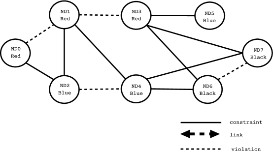
Consider the 3-coloring problem presented in figure 7. In this problem, there are 8 agents, each with a variable and 12 edges or constraints between them. Because this is a 3-coloring problem, each variable can only be assigned one of the three available colors {Black, Red, or Blue}. The goal is to find an assignment of colors to the variables such that no two variables, connected by an edge, have the same color.

In this example, four constraints are in violation: (ND0,ND1), (ND1,ND3), (ND2,ND4), and (ND6,ND7). Following the algorithm, upon startup each agent adds itself to its $good\_list$ and sends an “init” message to its neighbors. Upon receiving these messages, the agents add each of their neighbors to their $good\_list$ because they are able to identify a shared constraint with themselves.

Once the startup has been completed, each of the agents checks its $agent\_view$ . All of the agents, except ND5, find that they have conflicts. ND0 (priority 3) waits for ND1 to mediate (priority 5). ND6 and ND7, both priority 4, wait for ND4 (priority 5, tie with ND3 broken using lexicographical ordering). ND1, having an equal number of agents in its $good\_list$ , but a lower lexicographical order, waits for ND4 to start a mediation. ND3, knowing it is highest priority amongst its neighbors, first checks to see if it can resolve its conflict by changing its value, which in this case, it cannot. ND3 starts a session that involves ND1, ND5, ND6, and ND7. It sends each of them an “evaluate?” message. ND4 being highest priority amongst its neighbors, and unable to resolve its conflict locally, also starts a session by sending “evaluate?” messages to ND1, ND2, ND6, and ND7.

When each of the agents in the mediation receives the “evaluate?” message, they first check to see if they are expecting a mediation from a higher priority agent. In this case, ND1, ND6, and ND7 are expecting from ND4 so tell ND3 to wait. Then they label their domain elements with the names of the variables that they would be in conflict with as a result of adopting that value. This information is sent in an “evaluate!” message. The following are the labeled domains for the agents that are sent to ND4:

•

ND1 - Black causes no conflicts; Red conflicts with ND0 and ND3; Blue conflicts with ND2 and ND4
•

ND2 - Black causes no conflicts; Red conflicts with ND0 and ND3; Blue conflicts with ND4
•

ND6 - Black conflicts with ND7; Red conflicts with ND3; Blue conflicts with ND4
•

ND7 - Black conflicts with ND6; Red conflicts with ND3; Blue conflicts with ND4

The following are the responses sent to ND3:

•

ND1 - wait!
•

ND5 - Black causes no conflicts; Red conflicts with ND3; Blue causes no conflicts
•

ND6 - wait!
•

ND7 - wait!

Once all of the responses are received, the mediators, ND3 and ND4, conduct a branch and bound searches that attempt to find a satisfying assignment to their subproblems and minimizes the amount of conflict that would be created outside of the mediation. If either of them cannot find at least one satisfying assignment, it broadcasts that a solution cannot be found.

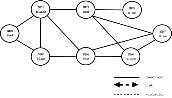
In this example, ND3, with the limited information that it has, computes a satisfying solution that changes its own color and to remain consistent would have also changed the colors of ND6 and ND7. Since it was told by ND6 and ND7 to wait, it changes its color, sends an “accept’!” message to ND5 and “ok?” messages to ND1, ND6 and ND7. Having more information, ND4 finds a solution that it thinks will solve its subproblem without creating outside conflicts. It changes its own color to red, ND7 to blue, and ND1 to black leaving the problem in the state shown in figure 8.

ND1, ND4, ND5, ND6 and ND7 inform the agents in their $agent\_view$ of their new values, then check for conflicts. This time, ND1, ND3, and ND6 notice that their values are in conflict. ND3, having the highest priority, becomes the mediator and mediates a session with ND1, ND5, ND6, and ND7. Following the protocol, ND3 sends out the “evaluate?” messages and the receiving agents label and respond. The following are the labeled domains that are returned:

•

ND1 - Black conflicts with ND3; Red conflicts with ND0 and ND4; Blue conflicts with ND2
•

ND5 - Black conflicts with ND3; Red causes no conflicts; Blue causes no conflicts
•

ND6 - Black conflicts with ND3; Red conflicts with ND4; Blue conflicts with ND7
•

ND7 - Black conflicts with ND3 and ND6; Red conflicts with ND4; Blue causes no conflicts

ND3, after receiving these messages, conducts its search and finds a solution that solves its subproblem. It chooses to change its color to red. ND1, ND3, ND5, ND6, and ND7 check their $agent\_view$ and find no conflicts. Since, at this point, none of the agents have any conflict, the problem is solved (see figure 9).

4.3 Soundness and Completeness

In this section we will show that the APO algorithm is both sound and complete. For these proofs, it is assumed that all communications are reliable, meaning that if a message is sent from $x_{i}$ to $x_{j}$ that $x_{j}$ will receive the message in a finite amount of time. We also assume that if $x_{i}$ sends message $m_{1}$ and then sends message $m_{2}$ to $x_{j}$ , that $m_{1}$ will be received before $m_{2}$ . Lastly, we assume that the centralized solver used by the algorithm is sound and complete. Before we prove the soundness and completeness, it helps to have a few principal lemmas established.

Lemma 1

Links are bidirectional. i.e. If $x_{i}$ has $x_{j}$ in its $agent\_view$ then eventually $x_{j}$ will have $x_{i}$ in its $agent\_view$ .

Proof:

Assume that $x_{i}$ has $x_{j}$ in its $agent\_view$ and that $x_{i}$ is not in the $agent\_view$ of $x_{j}$ . In order for $x_{i}$ to have $x_{j}$ in its $agent\_view$ , $x_{i}$ must have received an “init” message at some point from $x_{j}$ . There are two cases.

Case 1: $x_{j}$ is in the $initList$ of $x_{i}$ . In this case, $x_{i}$ must have sent $x_{j}$ an “init” message first, meaning that $x_{j}$ received an “init” message and therefore has $x_{i}$ in its $agent\_view$ , a contradiction.

Case 2: $x_{j}$ is not in the $initList$ of $x_{i}$ . In this case, when $x_{i}$ receives the “init” message from $x_{j}$ , it responds with an “init” message. That means that if the reliable communication assumption holds, eventually $x_{j}$ will receive $x_{i}$ ’s “init” message and add $x_{i}$ to its $agent\_view$ . Also a contradiction.

Lemma 2

If agent $x_{i}$ is linked to $x_{j}$ and $x_{j}$ changes its value, then $x_{i}$ will eventually be informed of this change and update its agent_view.

Proof:

Assume that $x_{i}$ has a value in its $agent\_view$ for $x_{j}$ that is incorrect. This would mean that at some point $x_{j}$ altered its value without informing $x_{i}$ . There are two cases:

Case 1: $x_{j}$ did not know it needed to send $x_{i}$ an update. i.e. $x_{i}$ was not in $x_{j}$ ’s $agent\_view$ . Contradicts lemma 1.

Case 2: $x_{j}$ did not inform all of the agents in its $agent\_view$ when it changes its value. It is clear from the code that this cannot happen. Agents only change their values in the check_agent_view, choose_solution, and accept! procedures. In each of these cases, it informs all of the agents within its $agent\_view$ by either sending an “ok?” or through the “accept!” message that a change to its value has occurred. A contradiction.

Lemma 3

If $x_{i}$ is in conflict with one or more of its neighbors, does not expect a mediation from another higher priority agent in its $agent\_view$ , and is currently not in a session, then it will act as mediator.

Proof:

Directly from the procedure check_agent_view.

Lemma 4

If $x_{i}$ mediates a session that has a solution, then each of the constraints between the agents involved in the mediation will be satisfied.

Proof:

Assume that there are two agents $x_{j}$ and $x_{k}$ (either of them could be $x_{i}$ ), that were mediated over by $x_{i}$ and after the mediation there is a conflict between $x_{j}$ and $x_{k}$ . There are two ways this could have happened.

Case 1: One or both of the agents must have a value that $x_{i}$ did not assign to it as part of the mediation.

Assume that $x_{j}$ and/or $x_{k}$ has a value that $x_{i}$ did not assign. We know that since $x_{i}$ mediated a session including $x_{j}$ and $x_{k}$ , that $x_{i}$ did not receive a “wait!” message from either of $x_{j}$ or $x_{k}$ . This means that they could not have been mediating. This also means that they must have set their $mediate$ flags to true when $x_{i}$ sent them the “evaluate?” message. Since the only times an agent can change its value is when its $mediate$ flag is false, it is mediating, or has been told to by a mediator, $x_{j}$ and/or $x_{k}$ could only have changed their values is if $x_{i}$ told them to, which contradicts the assumption.

Case 2: $x_{i}$ assigned them a value that caused them to be in conflict with one another.

Let’s assume that $x_{i}$ assigned them conflicting values. This means that $x_{i}$ chose a solution that did not take into account the constraints between $x_{j}$ and $x_{k}$ . But, we know that $x_{i}$ only chooses satisfying solutions that include all of the constraints between all of the agents in the $good\_list$ . This leads to a contradiction.

This lemma is important because it says that once a mediator has successfully concluded its session, the only conflicts that can exist are on constraints that were outside of the mediation. This can be viewed as the mediator pushing the constraint violations outside of its view. In addition, because mediators get information about who the violations are being pushed to and establish links with those agents, over time, they gain more context. This is a very important point when considering the completeness of the algorithm.

Theorem 1

The APO algorithm is sound. i.e. It reaches a stable state only if it has either found an answer or no solution exists.

Proof:

In order to be sound, the agents can only stop when they have reached an answer. The only condition in which they would stop without having found an answer is if one or more of the agents is expecting a mediation request from a higher priority agent that does not send it. In other words, the protocol has deadlocked.

Let’s say we have 3 agents, $x_{i}$ , $x_{j}$ , and $x_{k}$ with $p_{i}<p_{j}\vee p_{k}<p_{j}$ ( $i$ could be equal to $k$ ) and $x_{k}$ has a conflict with $x_{j}$ . There are two cases in which $x_{j}$ would not mediate a session that included $x_{i}$ , when $x_{i}$ was expecting it to:

Case 1: $x_{i}$ has $m_{j}={\bf true}$ in its $agent\_view$ when the actual value should be false.

Assume that $x_{i}$ has $m_{j}={\bf true}$ in its $agent\_view$ when the true value of $m_{j}={\bf false}$ . This would mean that at some point $x_{j}$ changed the value of $m_{j}$ to false without informing $x_{i}$ . There is only one place that $x_{j}$ changes the value of $m_{j}$ , this is in the check_agent_view procedure (see figure 3). Note that in this procedure, whenever the flag changes value from true to false, the agent sends an “ok” message to all the agents in its $agent\_view$ . Since by lemma 1 we know that $x_{i}$ is in the $agent\_view$ of $x_{j}$ , $x_{i}$ must have received the message saying that $m_{j}={\bf false}$ , contradicting the assumption.

Case 2: $x_{j}$ believes that $x_{i}$ should be mediating when $x_{i}$ does not believe it should be. i.e. $x_{j}$ thinks that $m_{i}={\bf true}$ and $p_{i}>p_{j}$ .

By the previous case, we know that if $x_{j}$ believes that $m_{i}={\bf true}$ that this must be the case. We only need to show that $p_{i}<p_{j}$ . Let’s say that $p^{\prime}_{i}$ is the priority that $x_{j}$ believes $x_{i}$ has and assume that $x_{j}$ believes that $p^{\prime}_{i}>p_{j}$ when, in fact $p_{i}<p_{j}$ . This means that at some point $x_{i}$ sent a message to $x_{j}$ informing it that its current priority was $p^{\prime}_{i}$ . Since we know that priorities only increase over time (the good_list only gets larger), we know that $p^{\prime}_{i}\leq p_{i}$ ( $x_{j}$ always has the correct value or underestimates the priority of $x_{i}$ ). Since $p_{j}>p_{i}$ and $p_{i}\geq p^{\prime}_{i}$ then $p_{j}>p^{\prime}_{i}$ which contradicts the assumption.

This is also an important point when considering how the algorithm behaves. This proof says that agents always either know or underestimate the true value of their neighbors’ priorities. Because of this, the agents will attempt to mediate when in fact sometimes, they shouldn’t. The side effect of this attempt, however, is that the correct priorities are exchanged so the same mistake doesn’t get repeated. The other important thing to mention is the case were the priority values become equal. In this case, the tie is broken by using the alphabetical order of names of the agents. This ensures that there is always a way to break ties.

Definition 1

Oscillation is a condition that occurs when a subset $V^{\prime}\subseteq V$ of the agents are infinitely cycling through their allowable values without reaching a solution. In other words, the agents are live-locked

By this definition, in order to be considered part of an oscillation, an agent within the subset must be changing its value (if it’s stable, it’s not oscillating) and it must be connected to the other members of the subset by a constraint (otherwise, it is not actually a part of the oscillation).

Theorem 2

The APO algorithm is complete. i.e. if a solution exists, the algorithm will find it. If a solution does not exist, it it will report that fact.

Proof:

A solution does not exist whenever the problem is over-constrained. If the problem is over-constrained, the algorithm will eventually produce a $good\_list$ where the variables within it and their associated constraints lead to no solution. Since a subset of the variables is unsatisfiable, the entire problem is unsatisfiable, therefore, no solution is possible. The algorithm terminates with failure if and only if this condition is reached.

Since we have now shown in Theorem 1 that whenever the algorithm reaches a stable state, the problem is solved and that when it finds a subset of the variables that is unsatisfiable it terminates, we only need to show that it reaches one of these two states in finite time. The only way for the agents to not reach a stable state is when one or more of the agents in the system is in an oscillation.

There are two cases to consider, the easy case is when a single agent is oscillating ( $|V^{\prime}|=1$ ) and the other case is when more than one agent is oscillating ( $|V^{\prime}|>1$ ).

Case 1: There is an agent $x_{i}$ that is caught in an infinite loop and all other agents are stable.

Let’s assume that $x_{i}$ is in an infinite processing loop. That means that no matter what it changes its value to, it is in conflict with one of its neighbors, because if it changed its value to something that doesn’t conflict with its neighbors, it would have a solution and stop. If it changes its value to be in conflict with some $x_{j}$ that is higher priority than it, then $x_{j}$ will mediate with $x_{i}$ , contradicting the assumption that all other agents are stable. If $x_{i}$ changes its value to be in conflict with a lower priority agent, then by lemma 3, it will act as mediator with its neighbors. Since it was assumed that each of the other agents is in a stable state, then all of the agents in $x_{i}$ ’s $good\_list$ will participate in the session and by lemma 4, agent $x_{i}$ will have all of its conflicts removed. This means that $x_{i}$ will be in a stable state contradicting the assumption that it was in an infinite loop.

Case 2: Two or more agents are in an oscillation.

Let’s say we have a set of agents $V^{\prime}\subseteq V$ that are in an oscillation. Now consider an agent $x_{i}$ that is within $V^{\prime}$ . We know that the only conditions in which $x_{i}$ changes its value is when it can do so and solve all of its conflicts (a contradiction because $x_{i}$ wouldn’t be considered part of the oscillation), as the mediator, or as the receiver of a mediation from some other agent in $V^{\prime}$ . The interesting case is when an agent acts as the mediator.

Consider the case when $x_{i}$ is the mediator and call the set of agents that it is mediating over $V_{i}$ . We know according to definition 1 that after the mediation, that at least one conflict must be created or remain otherwise the oscillation would stop and the problem would be solved. In fact, we know that each of the remaining conflicts must contain an agent from the set $V^{\prime}-V_{i}$ by lemma 4. We also know that for each violated constraint that has a member from $V_{i}$ , that $x_{i}$ will link with any agent that is part of those constraints and not a member of $V_{i}$ . The next time $x_{i}$ mediates, the set $V_{i}$ will include these members and the number of agents in the set $V^{\prime}-V_{i}$ is reduced. In fact, whenever $x_{i}$ mediates the set $V^{\prime}-V_{i}$ will be reduced (assuming it is not told to wait! by one or more agents. In this case, it takes longer to reduce this set, but the proof still holds). Eventually, after $O(|V|^{2})$ mediations, some $x_{i}$ within $V^{\prime}$ must have $V_{i}=V^{\prime}$ (every agent within the set must have mediated $|V^{\prime}|$ times in order for this to happen). When this agent mediates it will push the violations outside of the set $V^{\prime}$ or it will solve the subproblem by lemma 4. Either of these conditions contradicts the oscillation assumption. Therefore, the algorithm is complete. QED

It should be fairly clear that, in domains that are exponential, the algorithm’s worse-case runtime is exponential. The space complexity of the algorithm is, however, polynomial, because the agents only retain the names, priorities, values, and constraints of other agents.

5 Evaluation

A great deal of testing and evaluation has been conducted on the APO algorithm. Almost exclusively, these test are done comparing the APO algorithm with the currently fastest known, complete algorithm for solving DCSPs called the Asynchronous Weak Commitment (AWC) protocol. In this section we will describe the AWC protocol (section 5.1), then will describe the distributed 3-coloring domain and present results from extensive testing done in this domain (section 5.2). This testing compares these two algorithms across a variety of metrics, including the cycle time, number of messages, and serial runtime.

Next, we will describe the tracking domain (section 5.3) and present results from testing in this domain as well. For this domain, we modified the core search algorithm of APO to take advantage of the polynomial complexity of this problem. This variant called, APO-Flow, will also be described.

5.1 The Asynchronous Weak Commitment (AWC) Protocol

The AWC protocol (?) was one of the first algorithms used for solving DCSPs. Like the APO algorithm, AWC is based on variable decomposition. Also, like APO, AWC assigns each agent a priority value that dynamically changes. AWC, however, uses the weak-commitment heuristic (?) to assign these priorities values which is where it gets its name.

Upon startup, each of the agents selects a value for its variable and sends “ok?” messages to its neighbors (agents it shares a constraint with). This message includes the variables value and priority (they all start at 0).

When an agent receives an “ok?” message, it updates its $agent\_view$ and checks its nogood list for violated $nogoods$ . Each nogood is composed of a set of nogood pairs which describe the combination of agents and values that lead to an unsatisfiable condition. Initially, the only nogoods in an agent’s nogood list are the constraints on its variable.

When checking its nogood list, agents only check for violations of higher priority nogoods. The priority of a nogood is defined as the priority of the lowest priority variable in the nogood. If this value is greater than the priority of the agent’s variable, the nogood is higher priority. Based on the results from this check, one of three things can happen:

1.

If no higher priority nogoods are violated, the agent does nothing.
2.

If there are higher priority nogoods that are violated and this can be repaired by simply changing the agent’s variable value, then the agent changes its value and sends out “ok?” messages to the agents in its $agent\_view$ . If there are multiple possible satisfying values, then the agent chooses the one that minimizes the number of violated lower priority nogoods.
3.

If there are violated higher priority nogoods and this cannot be repaired by changing the value of its variable, the agent generates a new nogood. If this nogood is the same as a previously generated nogood, it does nothing. Otherwise, it then sends this new nogood to every agent that has a variable contained in the nogood and raises the priority value of its variable. Finally, it changes its variable value to one that causes the least amount of conflict and sends out “ok?” messages.

Upon receiving a nogood message from another agent, the agent adds the nogood to its nogood list and rechecks for nogood violations. If the new nogood includes the names of agents that are not in its $agent\_view$ it links to them. This linking step is essential to the completeness of the search(?), but causes the agents to communicate nogoods and ok? messages to agents that are not their direct neighbors in the constraint graph. The overall effect is an increase in messages and a reduction in the amount of privacy being provided to the agents because they communicate potential domain values and information about their constraints through the exchange of ok? and nogood messages with a larger number of agents.

One of the more recent advances to the AWC protocol has been the addition of resolvent-based nogood learning (?) which is an adaptation of classical nogood learning methods (?, ?, ?).

The resolvent method is used whenever an agent finds that it needs to generate a new nogood. Agents only generate new nogoods when each of their domain values are in violation with at least one higher priority nogood already in their nogood list. The resolvent method works by selecting one of these higher priority nogoods for each of the domain values and aggregating them together into a new nogood. This is almost identical to a resolvent in propositional logic which is why it is referred to as resolvent-based learning. The AWC protocol used for all of our testing incorporates resolvent-based nogood learning.

5.2 Distributed Graph Coloring

Following directly from the definition for a CSP, a graph coloring problem, also known as a $k$ -colorability problem, consists of the following:

•

a set of n variables $V=\{x_{1},\ldots,x_{n}\}$ .
•

a set of possible colors for each of the variables $D=\{D_{1},\ldots,D_{n}\}$ where each $D_{i}$ is has exactly $k$ allowable colors.
•

a set of constraints $R=\{R_{1},\ldots,R_{m}\}$ where each $R_{i}(d_{i},d_{j})$ is predicate which implements the “not equals” relationship. This predicate returns true iff the value assigned to $x_{i}$ differs from the value assigned to $x_{j}$ .

The problem is to find an assignment $A=\{d_{1},\ldots,d_{n}|d_{i}\in D_{i}\}$ such that each of the constraints in $R$ is satisfied. Like the general CSP, graph coloring has been shown to be NP-complete for all values of $k>2$ .

To test the APO algorithm, we implemented the AWC and APO algorithms and conducted experiments in the distributed 3-coloring domain. The distributed 3-coloring problem is a 3-coloring problem with n variables and m binary constraints where each agent is given a single variable. We conducted 3 sets of graph coloring based experiments to compare the algorithms’ computation and communication costs.

5.2.1 Satisfiable Graphs

In the first set of experiments, we created solvable graph instances with $m=2.0n$ (low-density), $m=2.3n$ (medium-density), and $m=2.7n$ (high-density) according to the method presented in (?). Generating graphs in this way involves partitioning the variables into $k$ equal-sized groups. Edges are then added by selecting two of the groups at random and adding an edge between a random member of each group. This method ensures that the resulting graphs are satisfiable, but also tests a very limited and very likely easier subset of the possible graphs. These tests were done because they are traditionally used by other researchers in DCSPs.

These particular values for $m$ were chosen because they represent the three major regions within the phase-transition for 3-colorability (?). A phase transition in a CSP is defined based on an order parameter, in this case the average node degree $d$ . The transition occurs at the point where random graphs created with that order value yield half satisfiable and half unsatisfiable instances. Values of the order parameter that are lower than the transition point (more than 50% of the instance are satisfiable) are referred to being to the left of the transition. The opposite is true of values to the right.

Phase transitions are important because that are strongly correlated with the overall difficulty of finding a solution to the graph (?, ?, ?). Within the phase transition, randomly created instances are typically difficult to solve. Interestingly, problems to the right and left of the phase transitions tend to be much easier.

In 3-colorability, the value $d=2.0$ is to the left of the phase transition. In this region, randomly created graphs are very likely to be satisfiable and are usually easy to find solve. At $d=2.3$ , which is in the middle of the phase transition the graph has about a 50% chance of being satisfiable and is usually hard to solve. For $m=2.7n$ , right of the phase transition, graphs are more than likely to be unsatisfiable and, again, are also easier to solve.

		APO	APO	AWC	AWC
$d$	Nodes	Mean	StDev	Mean	StDev	p( $AWC\leq APO$ )
	15	17.82	8.15	17.38	12.70	0.77
	30	27.07	17.11	24.62	19.23	0.27
2.0	45	39.97	25.79	43.76	30.98	0.34
	60	53.24	32.32	69.96	49.03	0.01
	75	59.83	35.35	80.32	103.76	0.07
	90	80.75	54.30	82.92	61.01	0.81
	Overall					0.01
	15	15.04	5.55	20.49	11.27	0.00
	30	34.01	16.81	41.30	29.58	0.04
2.3	45	47.72	26.58	109.99	74.85	0.00
	60	92.73	72.46	135.60	146.57	0.01
	75	114.02	75.84	185.84	119.94	0.00
	90	160.88	125.12	189.04	91.27	0.07
	Overall					0.00
	15	13.83	3.56	20.29	10.32	0.00
	30	27.28	10.10	39.99	24.08	0.00
2.7	45	42.47	18.01	62.92	35.23	0.00
	60	52.15	23.12	86.89	43.69	0.00
	75	64.54	26.26	104.09	46.62	0.00
	90	87.14	42.82	127.04	64.97	0.00
	Overall					0.00

Table 1: Comparison of the number of cycles needed to solve satisfiable 3-coloring problems of various sizes and densities by AWC and APO.

A number of papers (?, ?, ?) have reported that $m=2.7n$ is within the critical phase transition for 3-colorability. This seems to have been caused by a misinterpretation of previous work in this area(?). Although Cheeseman, Kanefsky, and Taylor reported that $m=2.7n$ was within the critical region for 3-colorability, they were using reduced graphs for their analysis.

A reduced graph is one in which the trivially colorable nodes and non-relevant edges have been removed. For example, one can easily remove any node with just two edges in a 3-coloring problem because it can always be trivially colored. Additionally, nodes that possess a unique domain element from their neighbors can also be easily removed.

In later work, Culberson and Gent identified the critical region as being approximately $d=2.3$ and therefore was included in our tests(?). One should note, however, that because phase transitions are typically done on completely random graphs and by its very definition involves both satisfiable and unsatisfiable instances, it is very hard to apply the phase-tranisition results to graphs created using the technique described at the beginning of the section because it only generates satisfiable instances. A detailed phase transition analysis has not been done on this graph generation technique and in fact, we believe that these graphs tend to be easier than randomly created satisfiable ones of the same size and order.

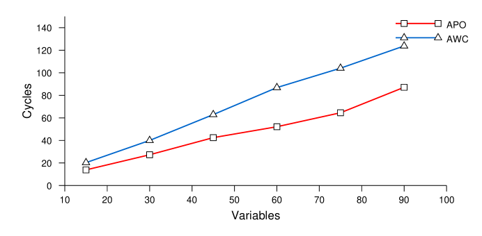
To evaluate the relative strengths and weakness of each of the approaches, we measured the number of cycles and the number of messages used during the course of solving each of the problems. During a cycle, incoming messages are delivered, the agent is allowed to process the information, and any messages that were created during the processing are added to the outgoing queue to be delivered at the beginning of the next cycle. The actual execution time given to one agent during a cycle varies according to the amount of work needed to process all of the incoming messages. The random seeds used to create each graph instance and variable instantiation were saved and used by each of the algorithms for fairness.

		% Links	% Links	% Central	% Central
	Nodes	Mean	StDev	Mean	StDev
	15	32.93	3.52	60.53	9.12
	30	17.24	2.59	42.53	8.06
APO	45	11.97	1.84	33.27	6.61
	60	9.30	1.30	29.00	7.31
	75	7.42	0.95	24.60	6.73
	90	6.51	0.96	24.93	6.16
	15	55.76	12.31	79.73	11.45
	30	32.89	8.88	60.97	10.98
AWC	45	27.00	7.89	56.49	11.57
	60	26.47	9.12	56.98	14.23
	75	21.99	7.67	53.19	13.29
	90	20.11	7.89	50.38	13.78

Table 2: Link statistics for satisfiable, low-density problems.

		% Links	% Links	% Central	% Central
	Nodes	Mean	StDev	Mean	StDev
	15	37.46	3.45	67.60	8.26
	30	21.24	2.85	51.37	9.32
APO	45	14.90	2.27	43.67	11.40
	60	12.85	2.99	42.98	13.06
	75	11.17	2.45	43.76	12.69
	90	10.07	3.10	40.47	14.55
	15	63.19	12.06	83.56	8.96
	30	42.84	11.83	72.20	12.09
AWC	45	52.05	13.52	80.67	11.24
	60	43.69	14.59	74.93	14.56
	75	47.77	14.10	79.41	12.18
	90	44.04	10.84	77.98	10.52

Table 3: Link statistics for satisfiable, medium-density problems.

		% Links	% Links	% Central	% Central
	Nodes	Mean	StDev	Mean	StDev
	15	43.28	2.86	74.53	8.34
	30	24.29	2.61	59.30	9.75
APO	45	18.07	2.06	52.62	10.21
	60	13.86	1.77	47.78	11.32
	75	11.85	1.57	46.37	11.32
	90	10.86	1.85	50.73	14.48
	15	78.87	12.29	93.60	7.75
	30	58.03	11.66	86.27	9.54
AWC	45	54.06	13.44	82.67	13.34
	60	53.01	12.77	83.47	11.04
	75	49.63	11.36	81.91	9.93
	90	47.72	13.81	80.32	15.06

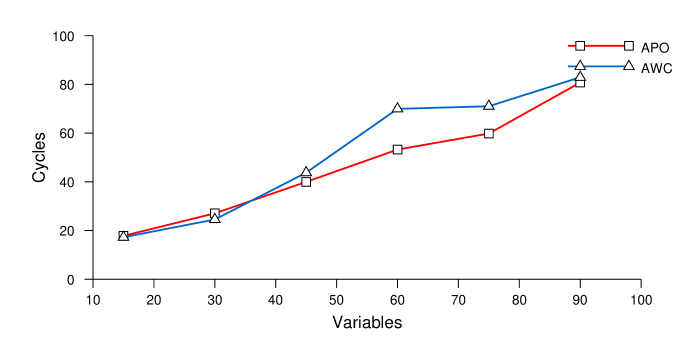
Table 4: Link statistics for satisfiable, high-density problems.

For this comparison between AWC and APO, we randomly generated 10 graphs of size $n=15,30,45,60,75,90$ and $m=2.0n,2.3n,2.7n$ and for each instance generated 10 initial variable assignments. Therefore, for each combination of $n$ and $m$ , we ran 100 trials making a total of 1800 trials. The results from this experiment can be seen in figures 10 through 15 and table 1. We should mention that the results of the testing on AWC obtained from these experiments agree with previous results (?) verifying the correctness of our implementation.

At first glance, figure 10 appears to indicate that for satisfiable low-density graph instances, AWC and APO perform almost identically in terms of cycles to completion. Looking at the associated table (Table 1), however, reveals that overall, the pairwise T-test indicates that with 99% confidence, APO outperforms AWC on these graphs.

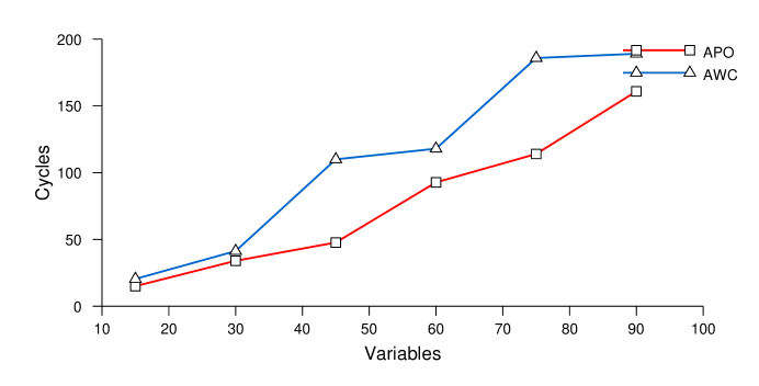
As the density, or average degree, of the graph increases, the difference becomes more apparent. Figures 11 and 12 show that APO begins to scale much more efficiently than AWC. This can be attributed to the ability of APO to rapidly identify strong interdependencies between variables and to derive solutions to them using a centralized search of the partial subproblem.

		APO	APO	AWC	AWC
$d$	Nodes	Mean	StDev	Mean	StDev	p( $AWC\leq APO$ )
	15	361.50	179.57	882.19	967.21	0.00
	30	1117.15	844.33	2431.71	3182.51	0.00
2.0	45	2078.72	1552.98	6926.86	7395.22	0.00
	60	3387.13	2084.69	18504.17	22281.59	0.00
	75	4304.22	2651.15	21219.01	22714.98	0.00
	90	6742.14	4482.54	33125.57	39766.56	0.00
	Overall					0.01
	15	379.15	188.69	1205.50	923.85	0.00
	30	1640.08	931.22	6325.21	6914.79	0.00
2.3	45	3299.05	2155.45	44191.89	44693.33	0.00
	60	8773.16	9613.84	70104.74	69050.66	0.00
	75	14368.87	12066.32	178683.02	173493.21	0.00
	90	25826.74	29172.66	201145.37	143236.26	0.00
	Overall					0.00
	15	433.64	164.12	1667.71	1301.03	0.00
	30	1623.89	787.59	9014.02	8104.34	0.00
2.7	45	3859.99	1921.51	28964.43	22900.89	0.00
	60	5838.36	3140.53	66857.87	53221.05	0.00
	75	9507.60	4486.04	116016.71	82857.63	0.00
	90	16455.59	10679.92	196239.22	163722.90	0.00
	Overall					0.00

Table 5: Comparison of the number of messages needed to solve satisfiable 3-coloring problems of various sizes and densities by AWC and APO.

		APO	APO	AWC	AWC
$d$	Nodes	Mean	StDev	Mean	StDev	p( $AWC\leq APO$ )
	15	10560.76	4909.09	11590.38	13765.19	0.49
	30	32314.97	23138.55	32409.93	45336.65	0.98
2.0	45	59895.10	42740.82	95061.77	106391.51	0.00
	60	97126.79	57428.70	259529.42	326087.70	0.00
	75	123565.94	73493.72	294502.71	328696.59	0.00
	90	192265.35	123384.05	466084.60	581963.72	0.00
	Overall					0.00
	15	11370.13	4951.75	16260.19	13237.31	0.00
	30	47539.20	25486.74	88946.59	101077.04	0.00
2.3	45	95098.49	59312.25	644007.01	675192.26	0.00
	60	247417.78	262844.89	1018059.11	1029273.23	0.00
	75	401618.24	327990.65	2626178.31	2606377.80	0.00
	90	712035.13	782835.83	2935211.45	2138087.17	0.00
	Overall					0.00
	15	13415.51	4280.15	22393.61	18578.25	0.00
	30	48542.24	21331.96	125072.76	116518.80	0.00
2.7	45	112541.02	52729.10	405535.81	327349.47	0.00
	60	170174.55	85705.12	945039.32	773937.60	0.00
	75	272391.95	122177.07	1641250.63	1204185.34	0.00
	90	465571.42	288265.82	2793725.78	2397839.47	0.00
	Overall					0.00

Table 6: Comparison of the number of bytes transmitted by APO and AWC for satisfiable graph instances of various sizes and density.

Tables 2 through 4, partially verify this statement. As you can see, on average, less than 50% of the possible number of links ( $n*(n-1)$ ) are used by APO in solving problems (% Links column). In addition, the maximum amount of centralization (% Central column) occuring within any single agent (i.e. the number of agents in its $agent\_view$ ) remains fairly low. The highest degree of centralization occurs for small, high-density graphs. Intuitively, this makes a lot of sense because in these graphs, a single node is likely to have a high degree from the very start. Combine this fact with the dynamic priority ordering and the result is large amounts of central problem solving.

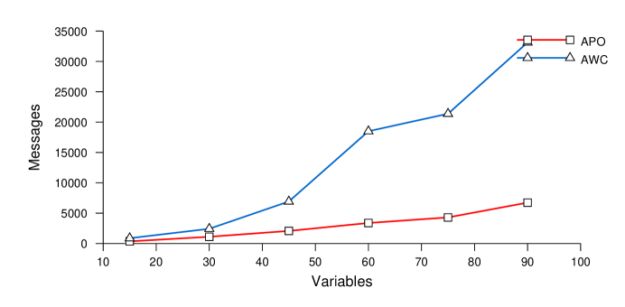
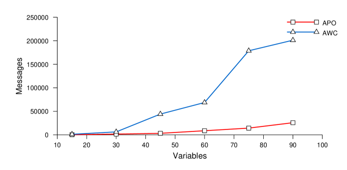
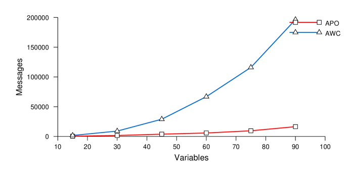
The most profound differences in the algorithms can be seen in figures 13, 14, and 15 and table 5. APO uses at least an order of magnitude less messages than AWC. Table 6 shows that these message savings lead to large savings in the number of bytes being transmitted as well. Even though APO uses about twice as many bytes per message as AWC (the messages were not optimized at all), the total amount of information be passed around is significantly less in almost every case.

Again, looking at the linking structure that AWC produces gives some insights into why it uses some many more messages than APO. Because agents communicate with all of the agents they are linked to whenever their value changes, and a large number of changes can occur in single cycle, AWC can have a tremendous amount of thrashing behavior. APO, on the other hand, avoids this problem because the process of mediating implicitly creates regions of stability in the problem landscape while the mediator decides on a solution. In addition, because APO uses partial centralization to solve problems, it avoids having to use a large number of messages to discover implied constraints through trial and error.

As we will see in the next two experiments, the high degree of centralization caused by its unfocused linking degrades AWC’s performance even more when solving randomly generated, possibly unsatisfiable, graph instances.

	APO	APO	% APO	AWC	AWC	% AWC
Density	Mean	StDev	Solved	Mean	StDev	Solved	$p(AWC\leq APO)$
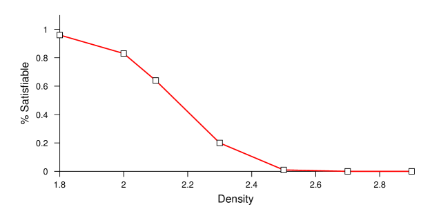
1.8	49.88	41.98	100	52.51	77.06	100	0.62
2.0	88.77	83.79	100	189.42	237.17	96	0.00
2.1	116.79	107.21	100	377.54	364.55	80	0.00
2.3	116.41	264.65	100	660.65	362.80	55	0.00
2.5	56.21	45.12	100	640.66	335.65	65	0.00
2.7	27.62	25.66	100	537.99	324.87	83	0.00
2.9	17.74	13.69	100	476.20	271.63	92	0.00
Overall							0.00

Table 7: Number of cycles needed to solve completely random 60 variable problems of various density using AWC and APO.

5.2.2 Random Graphs

In the second set of experiments, we generated completely random 60 node graphs with average degrees from $d=1.8$ to $2.9$ . This series was conducted to test the completeness of the algorithms, verify the correctness of their implementations, and to study the effects of the phase transition on their performance. For each value of $d$ , we generated 200 random graphs each with a single set of initial values. Graphs were generate by randomly choosing two nodes and connecting them. If the edge already existed, another pair was chosen. The phase transition curve for these instances can be seen in figure 16.

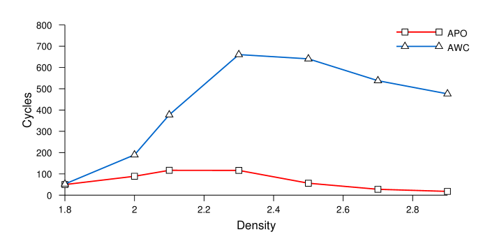
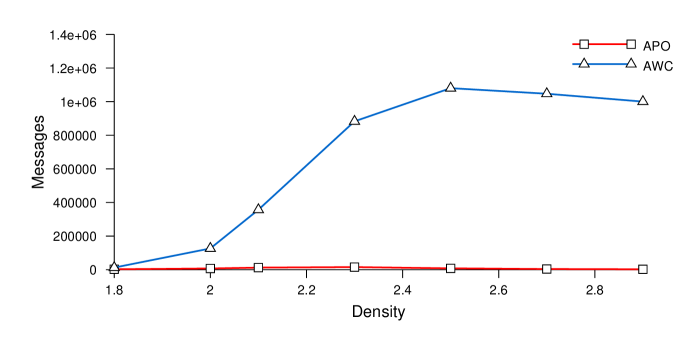
In total, 1400 graphs were generated and tested. Due to time constraints, we stopped the execution of AWC once 1000 cycles had completed (APO never reached 1000). The results of these experiments are shown in figures 17 and 18 and tables 7 and 8.

	APO	APO	AWC	AWC
Density	Mean	StDev	Mean	StDev	$p(AWC\leq APO)$
1.8	2822.61	3040.39	12741.58	47165.70	0.00
2.0	7508.33	9577.86	126658.29	269976.18	0.00
2.1	12642.68	16193.56	356993.39	444899.21	0.00
2.3	15614.37	15761.90	882813.45	566715.73	0.00
2.5	8219.74	7415.76	1080277.25	661909.63	0.00
2.7	4196.58	4201.80	1047001.18	738367.27	0.00
2.9	2736.20	2286.39	1000217.83	699199.90	0.00
Overall					0.00

Table 8: Number of messages needed to solve completely random 60 variable problems of various density using AWC and APO.

		% Links	% Links	% Central	% Central
	Density	Mean	StDev	Mean	StDev
	1.8	8.09	1.50	26.19	6.94
	2.0	10.93	3.28	36.92	13.77
	2.1	13.31	4.49	46.68	15.86
APO	2.3	15.56	4.94	55.91	18.18
	2.5	14.37	3.74	53.86	18.25
	2.7	13.19	3.32	47.33	19.59
	2.9	13.12	2.70	45.26	17.55
	1.8	16.28	6.58	41.08	12.42
	2.0	34.34	13.44	65.00	14.41
	2.1	46.52	13.95	75.24	10.66
AWC	2.3	64.13	11.43	86.06	5.61
	2.5	70.06	10.51	89.46	4.55
	2.7	72.95	10.65	91.71	3.80
	2.9	75.19	9.62	92.78	5.63

Table 9: Link statistics for 60 node random problems.

On these graphs, APO significantly outperforms AWC on all but the simplest problems (see figure 17). These results can most directly be attributed to AWC’s poor performance on unsatisfiable problem instances (?). In fact, in the region of the phase transition, AWC was unable to complete 45% of the graphs within the 1000 cycles.

In addition, to solve these problems, AWC uses at least an order of magnitude more messages that APO. These results can be seen in figure 18. By looking at table 9, it is easy to see why this occurs. AWC has a very high degree of linking and centralization. In fact, on $d=2.9$ graphs, AWC reaches an average of 93% centralization and 75% of complete inter-agent linking.

To contrast this, APO has very loose linking throughout the entire phase transition and centralizes on average around 50% of the entire problem. These results are very encouraging and reinforce the idea that partial overlays and extending along critical paths yields improvements in the convergence on solutions.

5.2.3 Runtime Tests

		APO	APO	AWC	AWC	BT	BT
$d$	Nodes	Mean	StDev	Mean	StDev	Mean	StDev
	15	0.26	0.21	2.72	4.40	0.02	0.02
2.0	30	0.78	0.66	10.52	18.99	1.65	4.14
	45	1.27	1.18	257.88	1252.25	245.14	587.31
	60	2.02	1.74	890.12	4288.43	27183.64	56053.26
	15	0.18	0.23	3.96	3.23	0.03	0.01
2.3	30	0.98	0.88	112.95	144.24	0.86	1.07
	45	2.19	2.26	1236.27	1777.51	150.73	241.02
	60	10.51	12.97	32616.24	62111.52	92173.71	222327.59
	15	0.09	0.06	3.51	2.90	0.02	0.01
2.7	30	0.40	0.39	61.43	59.77	0.29	0.36
	45	0.66	0.63	460.56	690.98	35.58	57.75
	60	5.47	5.44	4239.16	4114.30	2997.04	4379.97

Table 10: Comparison of the number of seconds needed to solve random 3-coloring problems of various sizes and densities using AWC, APO, and centralized Backtracking.

In the third set of experiments, we directly compared the serial runtime performance of AWC against APO. Serial runtime is measured using the following formula:

serialtime=\sum_{i=0}^{cycles}\sum_{a\in agents}time(a,i)

Which is just the total accumulated runtime needed to solve the problem when only one agent is allowed to process at a time.

For these experiments, we again generated random graphs, this time varying the size and the density of the graph. We generated 25 graphs for the values of $n=15,30,45,60$ and the densities of $d=2.0,2.3,2.7$ , for a total of 300 test cases. To show that the performance difference in APO and AWC was not caused by the speed of the central solver, we ran a centralized backtracking algorithm on the same graph instances. Although, APO uses the branch and bound algorithm, the backtracking algorithm used in this test provides a best case lower bound on the runtime of APO’s internal solver.

Each of the programs used in this test was run on an identical 2.4GHz Pentium 4 with 768 Mbytes of RAM. These machines where entirely dedicated to the tests so there was a minimal amount of interference by competing processes. In addition, no computational cost was assigned to message passing because the simulator passes messages between cycles. The algorithms were, however, penalized for the amount of time they took to process messages. Although we realize that the specific implementation of an algorithm can greatly effect its runtime performance, every possible effort was made to optimize the AWC implementation used for these experiments in an effort to be fair.

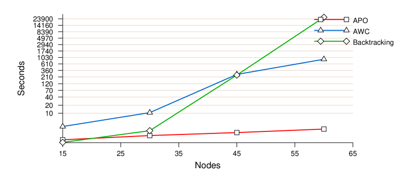
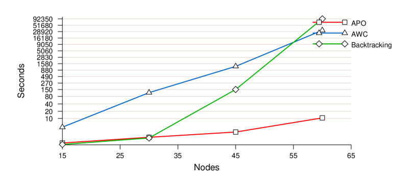
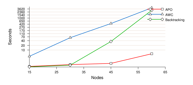
The results of this test series can be seen in figures 19, 20, and 21. You should note that the scale used for these graphs is logarithmic. From looking at these results, two things should become apparent. Obviously, the first is that APO outperforms AWC in every case. Second, APO actually outperforms its own centralized solver on graphs larger than 45 nodes. This indicates two things. First, the solver that is currently in APO is very poor and second that APO’s runtime performance is not a direct result of the speed of centralized solver that it is using. In fact, these tests show that the improved performance of APO over AWC is caused by APO’s ability to take advantage of the problem’s structure.

If we were to replace the centralized solver used in these tests with a state-of-the-art solver, we would expect two things. The first is that we would expect the serial runtime of the APO algorithm to decrease simply from the speedup caused by the centralized solver. The second, and more importantly, is that the centralized solver would always outperform APO. This is because current CSP solvers take advantage of problem structure unlike the solver used in these tests. We are in no way making a claim that APO improves any centralized solver. We are simply stating that APO outperforms AWC for reasons other than the speed of its current internal solver.

5.3 Tracking Domain

To test APO’s adaptability to various centralized solvers, we created an implementation of the complete-compatibility version of the SensorDCSP formulation (?, ?, ?). In this domain, there are a number of sensors and a number of targets randomly placed within an environment. Because of range restrictions, only sensors that are within some distance $dist$ can see a target. The goal is to find an assignment of sensors to targets such that each target has three sensors tracking it.

Following directly from the definition for a CSP, a SensorDCSP problem consists of the following:

•

a set of n targets $T=\{T_{1},\ldots,T_{n}\}$ .
•

a set of possible sensors that can “see” each of the targets $D=\{D_{1},\ldots,D_{n}\}$ .
•

a set of constraints $R=\{R_{1},\ldots,R_{m}\}$ where each $R_{i}(a_{i},a_{j})$ is predicate which implements the “not intersects” relationship. This predicate returns true iff the sensors assigned to $T_{i}$ does not have any elements in common with the sensors assigned to $T_{j}$ .

The problem is to find an assignment $A=\{a_{1},\ldots,a_{n}\}$ such that each of the constraints in $R$ is satisfied and each $a_{i}$ is a set of $|D_{i}|\choose c$ sensors from $D_{i}$ where $c=min(|D_{i}|,3)$ . This indicates that each target requires 3 sensors, if enough are available, or all of the sensors, if there are less than 3.

Since, in this implementation, each of the sensors is compatible with one another, the overall complexity of the problem is polynomial, using a reduction to feasible flow in a bipartite graph(?). Because of this, the centralized solver used by the APO agents was changed to a modified version of the Ford-Fulkerson maximum flow algorithm (?, ?), which has been proven to run in polynomial time.

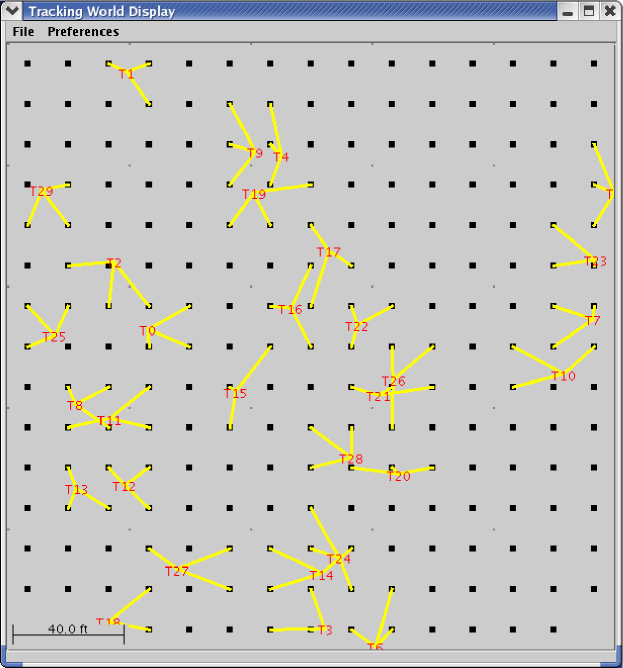
An example of the tracking problem can be seen in figure 22. In this example, there are 224 sensors (black dots) placed in an ordered pattern in the environment. There are 30 targets (labeled with their names) which are randomly placed at startup. The lines connecting sensors to targets indicate that the sensor is assigned to the target. Note that this instance of the problem is satisfiable.

5.3.1 Modifying APO for the Tracking Domain

Because the tracking domain is so closely related to the general CSP formulation, very few changes were made to either AWC or APO for these tests. We did, however, decide to test the adaptability of APO to a new centralized problem solver. To do this, we changed the centralized problem solver to the Ford Fulkerson max-flow algorithm in figure 23. Ford-Fulkerson works by repeatedly finding paths with remaining capacity through the residual flow network and augmenting the flows along those paths. The algorithm terminates when no additional paths can be found. A detailed explanation of the algorithm as well as a proof of its optimality can be found in (?).

Ford-Fulkerson $(G,s,t)$ for each edge $(u,v)\in E[G]$ do $f[u,v]\leftarrow 0$ ; $f[v,u]\leftarrow 0$ ; end do; while there exists a path $p$ from $s$ to $t$ in the residual network $G_{f}$ do $c_{f}(p)\leftarrow$ min $\{c_{f}(u,v):(u,v)\in p\}$ ; for each edge $(u,v)\in p$ do $f[u,v]\leftarrow f[u,v]+c_{f}(p)$ ; $f[v,u]\leftarrow-f[u,v]$ ; end do; end do; end Ford-Fulkerson;

Figure 23: The Ford-Fulkerson maximum flow algorithm.

Like mapping bipartite graphs into max-flow, the SensorDCSP problem is also easily mapped into max-flow. In figures 24 and 25 you can see the mapping of a simple sensor allocation problem into a max-flow problem. Notice that the capacity of the flow between the sensors and targets is 1. This ensures that a sensor cannot be used by more than a single target. Also, notice that the capacity of the targets to $t$ is 3. In fact, this value is to min $(|D_{i}|,3)$ .

To use this algorithm within APO, the mediator simply translates the problem into a network flow graph $G$ using the following rules whenever it runs the choose_solution procedure in figure 5:

1.

Add the nodes $s$ and $t$ to $G$ .
2.

For each $T_{i}\in T$ add a node $T_{i}$ and an edge $(T_{i},t)$ with capacity min $(|D_{i}|,3)$ to $G$ .
3.

For each unique sensor $S_{i}$ in the domains of $T_{i}\in T$ , add a node $S_{i}$ , an edge $(s,S_{i})$ with capacity 1, and an edge $(S_{i},T_{i})$ with capacity 1 to $G$ .

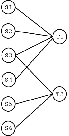
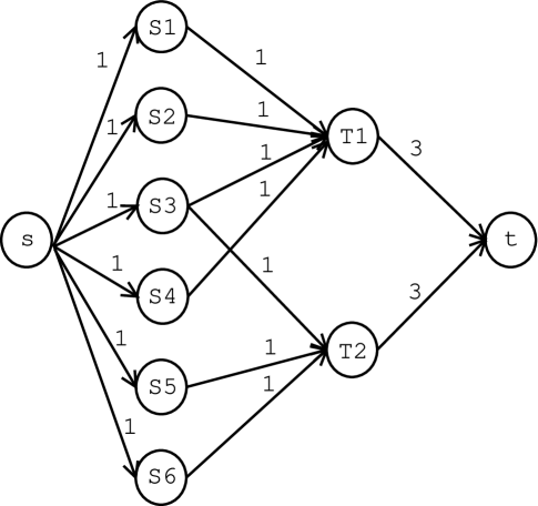
It then executes the Ford-Fulkerson algorithm. Once the algorithm finishes, the mediator checks the residual capacity of the edges between the targets and $t$ . If any of these edges has residual flow, then the problem is unsatisfiable. Otherwise, the assignment can be derived by finding all of the $(S_{i},T_{i})$ edges that have a flow of 1.

One of the nicest characteristics of the Ford-Fulkerson algorithm is that it works regardless of the order that the paths in the residual network are chosen. In our implementation, we used a breadth-first search which, in addition to identifying paths in the residual network, minimized the cost of the path. Cost in this sense refers to the amount of external conflict that is created by having a sensor assigned to a target. This modification maintains the min-conflict heuristic which is an integral part of extending the mediators local view.

5.3.2 Results

To test APO and AWC in this domain, we ran a test series which used a $200ft\times 200ft$ environment with 224 sensors placed in an ordered grid-based pattern. We chose to place the sensors in an ordered fashion to reduce the variance obtained within the results. We ran a test series which varied the sensor to target ratio from 10:1 to 3.8:1 (22 to 59 targets) in increments of 0.2 which is across the spectrum from mostly satisfiable to mostly unsatisfiable instances (see figure 26). We then conducted 250 trial runs with a random target placement for each of these values to get a good statistical sampling.

In total, 6750 test cases were used. For comparison, we measured the number of messages and cycles that were taken by the algorithms to find a solution. The random seeds used to place the targets were saved, so APO and AWC were both tested using identical problem instances. The correctness of the algorithms was verified by cross-checking the solutions (satisfiable/unsatisfiable) obtained during these tests, which matched identically.

As can be seen in figure 27 and 28 and tables 11 and 12, APO outperforms AWC on all but the simplest cases. Part of the reason for this is the minimum 3 cycles it takes APO to finish a mediation session. In problems that have very sparsely connected interdependencies, this cost tends to dominate. All-in-all, as the T-tests indicate, APO is significantly better than AWC in terms of both cycles to completion and number of messages used for problems in this domain.

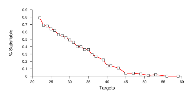
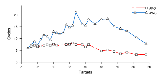
	APO	APO	AWC	AWC
Targets	Mean	StDev	Mean	StDev	$p(AWC\leq APO)$
22	6.36	2.33	5.88	6.61	0.29
23	6.65	3.39	7.32	10.55	0.36
24	7.12	4.72	8.83	19.96	0.18
25	6.55	3.24	7.15	10.56	0.39
26	6.80	4.28	9.65	15.78	0.01
27	7.09	5.02	10.85	19.89	0.00
28	7.38	5.88	11.05	15.89	0.00
29	7.10	4.89	9.24	13.76	0.02
30	7.55	5.99	13.15	25.58	0.00
31	7.18	6.11	12.42	22.22	0.00
32	6.88	6.31	11.73	18.21	0.00
33	7.62	7.59	12.32	24.04	0.00
34	7.47	7.81	15.88	28.82	0.00
35	7.56	7.49	14.74	29.01	0.00
36	8.08	9.89	15.70	25.46	0.00
37	7.48	8.38	20.70	39.63	0.00
39	7.55	10.87	16.12	26.43	0.00
40	6.45	10.54	15.74	21.66	0.00
41	7.45	13.11	17.56	30.98	0.00
43	5.96	7.79	16.10	22.91	0.00
45	4.80	7.25	17.61	28.50	0.00
47	5.15	8.31	18.52	30.27	0.00
49	4.53	5.90	15.33	25.28	0.00
51	3.52	2.00	14.34	22.60	0.00
53	4.12	5.82	13.13	22.55	0.00
56	3.14	0.59	10.45	20.81	0.00
59	3.28	2.26	7.46	10.47	0.00
Overall					0.00

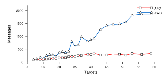
Table 11: Number of cycles needed to solve random target configurations in a field of 224 sensors using AWC and APO.

	APO	APO	AWC	AWC
Targets	Mean	StDev	Mean	StDev	$p(AWC\leq APO)$
22	78.28	32.58	95.68	133.53	0.04
23	89.52	54.01	133.12	237.74	0.00
24	105.53	90.36	184.19	616.36	0.04
25	102.92	57.18	149.18	298.85	0.02
26	116.36	86.58	245.99	566.03	0.00
27	128.58	98.63	263.32	587.30	0.00
28	149.23	144.81	279.49	493.05	0.00
29	145.72	93.24	231.98	335.98	0.00
30	167.50	144.27	378.89	874.99	0.00
31	169.30	152.83	404.40	997.82	0.00
32	174.32	152.89	362.63	570.41	0.00
33	212.59	237.60	410.05	923.25	0.00
34	218.74	246.18	811.58	2243.79	0.00
35	221.93	230.44	613.64	1422.33	0.00
36	258.41	354.13	671.00	1333.50	0.00
37	258.95	342.97	947.95	2116.98	0.00
39	303.64	501.10	815.32	1373.29	0.00
40	293.24	649.42	884.32	1407.99	0.00
41	342.33	724.64	912.65	1517.10	0.00
43	274.39	267.95	1279.97	2194.84	0.00
45	277.26	414.19	1334.38	2470.13	0.00
47	311.91	405.1	1471.82	2172.13	0.00
49	303.66	299.13	1487.65	2503.62	0.00
51	269.37	110.57	1571.46	2157.52	0.00
53	333.42	390.08	1804.47	2815.94	0.00
56	296.36	45.54	1895.23	3731.98	0.00
59	339.21	202.98	1765.18	3676.16	0.00
Overall					0.00

Table 12: Number of messages needed to solve random target configurations targets in a field of 224 sensors using AWC and APO.

6 Conclusions and Future Directions

In this article, we presented a new complete, distributed constraint satisfaction protocol called Asynchronous Partial Overlay (APO). Like AWC, APO allows the agents to retain their autonomy because they can obscure or completely hide internal variables and constraints. In addition, agents can refuse solutions posed by a mediator, instead taking over as the mediator if for some reason they are unhappy with a proposed solution. We also presented an example of its execution on a simple problem (section 4.2) and proved the soundness and completeness of the algorithm (section 4.3). Through extensive empirical testing on 10,250 graph instances from the graph coloring and tracking domain, we also showed that APO significantly outperforms the currently best known distributed constraint satisfaction algorithm, AWC (?). These tests have shown that APO is better than AWC in terms of cycles to completion, message usage, and runtime performance. We have also shown that the runtime characteristics can not be directly attributed to the speed of the centralized solver.

APO’s performance enhancements can be attributed to a number of things. First, APO exhibits a hill-climbing nature early in the search which becomes more focused and controlled as time goes on. Like other hill-climbing techniques this often leads to a satisfiable solution early in the search. Second, by using partial overlaying of the information that the agents use in decision making, APO exploits the work that has been previously done by other mediators. This forms a lock and key mechanism which promotes solution stability. Lastly, and most importantly, because APO uses dynamic, partial centralization, the agents work on smaller, highly relevant portions of the overall problem. By identifying these areas of decomposability, the search space can be greatly reduced which, in some cases, improves the efficiency of the centralized search algorithm.

There are a vast number of improvements planned for APO in the future. Probably the most important is to improve the centralized solver that it uses. In this article, an inefficient solver was chosen to show the strengths of the distributed portions of APO. We expect that additional improvements in the algorithm’s runtime performance can be obtained by using a faster centralized search engine. In addition, modern solvers often use methods like graph reductions, unit propagation and backbone guided search. It is conceivable that information gained from the centralized search engine could be used to prune the domains from the variables for consistency reasons and variables from the centralized subproblem for relevance reasons. We expect this will further focus the efforts of the agents additionally reducing the search time and communications usage of the algorithm.

Along with these improvements is the selective use of memory for recording nogoods. Unlike AWC which uses the nogoods to ensure a complete search, APO’s completeness relies on one of the agents centralizing the entire problem in the worst case. Because of this key difference, APO can be improved by simply remembering a small, powerful subset of the nogoods that it discovers from mediation session to session. This would allow the algorithm to improve future search by exploiting work that it had done previously.

What should be clear is that APO, and the cooperative mediation methodology as a whole, opens up new areas for future exploration and new questions to be answered in distributed problem solving. We believe that this work shows a great deal of promise for addressing a vast number of problems and represents a bridge between centralized and distributed problem solving techniques.

Acknowledgments

Special thanks to Bryan Horling for his design and implementation of the Farm simulation environment in which the experiment were run and to Shlomo Zilberstein, Bart Selman, Neil Immerman, and Jose Vidal for making numerous suggestions during the development of this work. Lastly, the authors would like to thank the JAIR reviewers for their helpful feedback and suggestions and Carlos Ansotegui and Jean-Charles Régin for their lengthy discussion during the final revision to this article.

The effort represented in this paper has been sponsored by the Defense Advanced Research Projects Agency (DARPA) and Air Force Research Laboratory, Air Force Materiel Command, USAF, under agreement number F30602-99-2-0525. The views and conclusions contained herein are those of the authors and should not be interpreted as necessarily representing the official policies or endorsements, either expressed or implied, of the Defense Advanced Research Projects Agency (DARPA), Air Force Research Laboratory, or the U.S. Government. The U.S. Government is authorized to reproduce and distribute reprints for Governmental purposes notwithstanding any copyright annotation thereon.

References

Bejar et al. Bejar, R., Krishnamachari, B., Gomes, C., & Selman, B. (2001). Distributed constraint satisfaction in a wireless sensor tracking system. In Workshop on Distributed Constraint Reasoning, International Joint Conference on Artificial Intelligence, Seattle, Washington.
Cammarata et al. Cammarata, S., McArthur, D., & Steeb, R. (1983). Strategies of cooperation in distributed problem solving. In Proceedings of the 8th International Joint Conference on Artificial Intelligence (IJCAI-83), Vol. 2, pp. 767–770.
Cha & Iwana Cha, B., & Iwana, K. (1996). Adding new clauses for faster local search. In Proceedings of the Thirteenth National Conference on Artificial Intelligence (AAAI), pp. 332–337.
Cheeseman et al. Cheeseman, P., Kanefsky, B., & Taylor, W. (1991). Where the really hard problems are. In Proceedings of the 12th International Joint Conference on Artificial Intelligence (IJCAI-91), pp. 331–337.
Conry et al. Conry, S. E., Kuwabara, K., Lesser, V. R., & Meyer, R. A. (1991). Multistage negotiation for distributed constraint satisfaction. IEEE Transactions on Systems, Man, and Cybernetics, 21(6).
Cormen et al. Cormen, T. H., Leiserson, C. E., & Rivest, R. L. (1999). Introduction to Algorithms. McGraw-Hill.
Culberson & Gent Culberson, J., & Gent, I. (2001). Frozen development in graph coloring. Theoretical Computer Science, 265(1–2), 227–264.
Fernandez et al. Fernandez, C., Bejar, R., Krishnamachari, B., Gomes, C., & Selman, B. (2003). Distributed Sensor Networks: A Multiagent Perspective, chap. Communication and Computation in Distributed CSP Algorithms, pp. 299–317. Kluwer Academic Publishers.
Ford & Fulkerson Ford, L. R., & Fulkerson, D. (1962). Flows in Networks. Princeton University Press.
Freuder & Wallace Freuder, E. C., & Wallace, R. J. (1992). Partial constraint satisfaction. Artificial Intelligence, 58(1–3), 21–70.
Frost & Dechter Frost, D., & Dechter, R. (1994). Dead-end driven learning. In Proceedings of the Twelfth Natioanl Conference on Artificial Intelligence, pp. 294–300.
Ginsberg Ginsberg, M. L. (1993). Dynamic backtracking. Journal of Artificial Intelligence Research, 1, 25–46.
Hayden et al. Hayden, S., Carrick, C., & Yang, Q. (1999). Architectural design patterns for multi-agent coordination. In Proceedings of the International Conference on Agent Systems, Seattle, WA.
Hirayama & Yokoo Hirayama, K., & Yokoo, M. (2000). The effect of nogood learning in distributed constraint satisfaction. In The 20th International Conference on Distributed Computing Systems (ICDCS), pp. 169–177.
Krishnamachari et al. Krishnamachari, B., Bejar, R., & Wicker, S. (2002). Distributed problem solving and the boundaries of self-configuration in multi-hop wireless networks. In Hawaii International Conference on System Sciences (HICSS-35).
Krishnamachari Krishnamachari, B. (2002). Phase Transitions, Structure, and Compleixty in Wireless Networks. Ph.D. thesis, Cornell University, Ithaca, NY.
Mammen & Lesser Mammen, D. L., & Lesser, V. R. (1998). Problem Structure and Subproblem Sharing in Multi-Agent Systems. Third International Conference on Multi-Agent Systems, 174–181.
Merriam-Webster Merriam-Webster (Ed.). (1995). The Merriam-Webster Dictionary (Home and Office edition). Springfield, IL.
Minton et al. Minton, S., Johnston, M. D., Philips, A. B., & Laird, P. (1992). Minimizing conflicts: A heuristic repair method for constraint satisfaction and scheduling problems. Artificial Intelligence, 58(1-3), 161–205.
Monasson et al. Monasson, R., Zecchina, R., Kirkpatrick, S., Selman, B., & Troyansky, L. (1999). Determining computational complexity from characteristic ’phase transitions’. Nature, 400, 133–137.
Rao & Kumar Rao, V. N., & Kumar, V. (1993). On the efficiency of parallel backtracking. IEEE Transactions on Parallel and Distributed Systems, 4(4), 427–437.
Sycara et al. Sycara, K., Roth, S., Sadeh, N., & Fox, M. (1991). Distributed constrained heuristic search. IEEE Transactions on Systems, Man, and Cybernetics, 21(6), 1446–1461.
Sycara Sycara, K. (1988). Resolving goal conflicts via negotiation. In Proceedings of the Seventh National Conference on Artificial Intelligence, pp. 245–250.
Wellman & Walsh Wellman, M., & Walsh, W. (1999). Distributed quiescence detection in multiagent negotiation. In In AAAI-99 Workshop on Negotiation: Settling Conflicts and Identifying Opportunities.
Werkman Werkman, K. J. (1990). Knowledge-based model of negotiation using shared perspectives. In Proceedings of the 10th International Workshop on Distributed Artificial intelligence, Bandera, TX.
Yokoo Yokoo, M. (1994). Weak-commitment search for solving constraint satisfaction problems. In Proceedings of the 12th National Conference on Artificial Intelligence (AAAI-94); Vol. 1, pp. 313–318, Seattle, WA, USA. AAAI Press, 1994.
Yokoo Yokoo, M. (1995). Asynchronous weak-commitment search for solving distributed constraint satisfaction problems.. In Proceedings of the First International Conference on Principles and Practice of Constraint Programming (CP-95), Lecture Notes in Computer Science 976, pp. 88–102. Springer-Verlag.
Yokoo et al. Yokoo, M., Durfee, E. H., Ishida, T., & Kuwabara, K. (1992). Distributed constraint satisfaction for formalizing distributed problem solving. In International Conference on Distributed Computing Systems, pp. 614–621.
Yokoo & Hirayama Yokoo, M., & Hirayama, K. (1996). Distributed breakout algorithm for solving distributed constraint satisfaction problems.. In International Conference on Multi-Agent Systems (ICMAS).
Yokoo & Hirayama Yokoo, M., & Hirayama, K. (2000). Algorithms for distributed constraint satisfaction: A review. Autonomous Agents and Multi-Agent Systems, 3(2), 198–212.
Yokoo et al. Yokoo, M., Suzuki, K., & Hirayama, K. (2002). Secure distributed constraint satisfaction: Reaching agreement without revealing private information. In Proceeding of the Eighth International Conference on Principles and Practice of Constraint Programming (CP).

Asynchronous Partial Overlay: A New Algorithm for Solving Distributed Constraint Satisfaction Problems

Abstract

1 Introduction

2 Distributed Constraint Satisfaction

3 Assumptions and Motivation

3.1 Assumptions

3.2 Motivation for Mediation-Based Problem Solving

4 Asynchronous Partial Overlay

4.1 The Algorithm

4.1.1 Initialization (Figure 2)

4.1.2 Checking the agent view (Figure 3)

4.1.3 Mediation (Figures 4, 5, and 6)

4.1.4 Multiple Variables and n𝑛n-ary Constraints

4.2 An Example

4.3 Soundness and Completeness

Lemma 1

Lemma 2

Lemma 3

Lemma 4

Theorem 1

Definition 1

Theorem 2

5 Evaluation

5.1 The Asynchronous Weak Commitment (AWC) Protocol

5.2 Distributed Graph Coloring

5.2.1 Satisfiable Graphs

5.2.2 Random Graphs

5.2.3 Runtime Tests

5.3 Tracking Domain

5.3.1 Modifying APO for the Tracking Domain

5.3.2 Results

6 Conclusions and Future Directions

References

4.1.4 Multiple Variables and $n$ -ary Constraints