Hamilton–Jacobi Theory for Degenerate Lagrangian Systems with Holonomic and Nonholonomic Constraints

Abstract

We extend Hamilton–Jacobi theory to Lagrange–Dirac (or implicit Lagrangian) systems, a generalized formulation of Lagrangian mechanics that can incorporate degenerate Lagrangians as well as holonomic and nonholonomic constraints. We refer to the generalized Hamilton–Jacobi equation as the Dirac–Hamilton–Jacobi equation. For non-degenerate Lagrangian systems with nonholonomic constraints, the theory specializes to the recently developed nonholonomic Hamilton–Jacobi theory. We are particularly interested in applications to a certain class of degenerate nonholonomic Lagrangian systems with symmetries, which we refer to as weakly degenerate Chaplygin systems, that arise as simplified models of nonholonomic mechanical systems; these systems are shown to reduce to non-degenerate almost Hamiltonian systems, i.e., generalized Hamiltonian systems defined with non-closed two-forms. Accordingly, the Dirac–Hamilton–Jacobi equation reduces to a variant of the nonholonomic Hamilton–Jacobi equation associated with the reduced system. We illustrate through a few examples how the Dirac–Hamilton–Jacobi equation can be used to exactly integrate the equations of motion.

I Introduction

I.1 Degenerate Lagrangian Systems and Lagrange–Dirac Systems

Degenerate Lagrangian systems are the motivation behind the work of Dirac (1950, 1958, 1964) on constrained systems, where degeneracy of Lagrangians imposes constraints on the phase space variables. The theory gives a prescription for writing such systems as Hamiltonian systems, and is used extensively for gauge systems and their quantization (see, e.g., Henneaux and Teitelboim (1992)).

Dirac’s theory of constraints was geometrized by Gotay et al. (1978) (see also Gotay and Nester (1979a, b, 1980) and Künzle (1969)) to yield a constraint algorithm to identify the solvability condition for presymplectic systems and also to establish the equivalence between Lagrangian and Hamiltonian descriptions of degenerate Lagrangian systems. The algorithm is extended by de León and Martín de Diego (1997) to degenerate Lagrangian systems with nonholonomic constraints.

On the other hand, Lagrange–Dirac (or implicit Lagrangian) systems of Yoshimura and Marsden (2006a, b) provide a rather direct way of describing degenerate Lagrangian systems that do not explicitly involve constraint algorithms. Moreover, the Lagrange–Dirac formulation can address more general constraints, particularly nonholonomic constraints, by directly encoding them in terms of Dirac structures, as opposed to symplectic or Poisson structures.

I.2 Hamilton–Jacobi Theory for Constrained Degenerate Lagrangian Systems

The goal of this paper is to generalize Hamilton–Jacobi theory to Lagrange–Dirac systems. The challenge in doing so is to generalize the theory to simultaneously address degeneracy and nonholonomic constraints. For degenerate Lagrangian systems, some work has been done, built on Dirac’s theory of constraints, on extending Hamilton–Jacobi theory (see, e.g., Henneaux and Teitelboim (1992)[Section 5.4] and Rothe and Scholtz (2003)) as well as from the geometric point of view by Cariñena et al. (2006). For nonholonomic systems, Iglesias-Ponte et al. (2008) generalized the geometric Hamilton–Jacobi theorem (see Theorem 5.2.4 of Abraham and Marsden (1978)) to nonholonomic systems, which has been studied further by de León et al. (2010), Ohsawa and Bloch (2009), Cariñena et al. (2010), and Ohsawa et al. (2011). However, to the authors’ knowledge, no work has been done that can deal with both degeneracy and nonholonomic constraints.

I.3 Applications to Degenerate Lagrangian Systems with Nonholonomic Constraints

We are particularly interested in applications to degenerate Lagrangian systems with nonholonomic constraints. Such systems arise regularly, in practice, as model reductions of multiscale systems: For example, consider a nonholonomic mechanical system consisting of rigid bodies, some of which are significantly lighter than the rest. Then, one can make an assumption that the light parts are massless for the sake of simplicity; this often results in a degenerate Lagrangian. While naïvely making a massless approximation usually leads to unphysical results, a certain class of nonholonomic systems seem to allow massless approximations without such inconsistencies. See, for example, the modelling of a bicycle in Getz (1994) and Getz and Marsden (1995) (see also Koon and Marsden (1997) and Example III.6 of the present paper).

I.4 Outline

We first briefly review Dirac structures and Lagrange–Dirac systems in Section II. Section III introduces a class of degenerate nonholonomic Lagrangian systems with symmetries that reduce to non-degenerate Lagrangian systems after symmetry reduction; we call them weakly degenerate Chaplygin systems. Section IV gives Hamilton–Jacobi theory for Lagrange–Dirac systems, defining the Dirac–Hamilton–Jacobi equation, and shows applications to degenerate Lagrangian systems with holonomic and nonholonomic constraints. We then apply the theory to weakly degenerate Chaplygin systems in Section V; we derive a formula that relates solutions of the Dirac–Hamilton–Jacobi equations with those of the nonholonomic Hamilton–Jacobi equation for the reduced weakly degenerate Chaplygin systems. Appendix A discusses reduction of weakly degenerate Chaplygin systems by a symmetry reduction of the associated Dirac structure.

II Lagrange–Dirac Systems

Lagrange–Dirac (or implicit Lagrangian) systems are a generalization of Lagrangian mechanics to systems with (possibly) degenerate Lagrangians and constraints. Given a configuration manifold $Q$, a Lagrange–Dirac system is defined using a generalized Dirac structure on $T^{*}Q$, or more precisely a subbundle $D$ of the Whitney sum $TT^{*}Q\oplus T^{*}T^{*}Q$.

II.1 Dirac Structures

Let us first recall the definition of a (generalized) Dirac structure on a manifold $M$. Let $M$ be a manifold. Given a subbundle $D\subset TM\oplus T^{*}M$, the subbundle $D^{\perp}\subset TM\oplus T^{*}M$ is defined as follows:

$$D^{\perp}\mathrel{\mathop{:}}=\left\{(X,\alpha)\in TM\oplus T^{*}M\ |\ \left\langle\alpha^{\prime},X\right\rangle+\left\langle\alpha,X^{\prime}\right\rangle=0\text{ for any $(X^{\prime},\alpha^{\prime})\in D$}\right\}.$$

Definition II.1.

A subbundle $D\subset TM\oplus T^{*}M$ is called a generalized Dirac structure if $D^{\perp}=D$.

Note that the notion of Dirac structures, originally introduced in Courant (1990), further satisfies an integrability condition, which we have omitted as it is not compatible with our interest in nonintegrable (nonholonomic) constraints. Hereafter, we refer to generalized Dirac structures as simply “Dirac structures.”

II.2 Induced Dirac Structures

Here we consider the induced Dirac structure $D_{\Delta_{Q}}\subset TT^{*}Q\oplus T^{*}T^{*}Q$ introduced in Yoshimura and Marsden (2006a). See Dalsmo and van der Schaft (1998) for more general Dirac structures, Bloch and Crouch (1997) and van der Schaft (1998) for those defined by Kirchhoff current and voltage laws, and van der Schaft (2006) for applications of Dirac structures to interconnected systems.

Let $Q$ be a smooth manifold, $\Delta_{Q}\subset TQ$ a regular distribution on $Q$, and $\Omega$ the canonical symplectic two-form on $T^{*}Q$. Denote by $\Delta_{Q}^{\circ}$ the annihilator of $\Delta_{Q}$ and by $\Omega^{\flat}:TT^{*}Q\to T^{*}T^{*}Q$ the flat map induced by $\Omega$. The distribution $\Delta_{Q}\subset TQ$ may be lifted to the distribution $\Delta_{T^{*}Q}$ on $T^{*}Q$ defined as

$$\Delta_{T^{*}Q}\mathrel{\mathop{:}}=(T\pi_{Q})^{-1}(\Delta_{Q})\subset TT^{*}Q,$$

where $\pi_{Q}:T^{*}Q\to Q$ is the canonical projection and $T\pi_{Q}:TT^{*}Q\to TQ$ is its tangent map. Denote its annihilator by $\Delta^{\circ}_{T^{*}Q}\subset T^{*}T^{*}Q$.

Definition II.2 (Yoshimura and Marsden (2006a, b); see also Dalsmo and van der Schaft (1998)).

The induced (generalized) Dirac structure $D_{\Delta_{Q}}$ on $T^{*}Q$ is defined, for each $z\in T^{*}Q$, as

$$D_{\Delta_{Q}}(z)\mathrel{\mathop{:}}=\left\{(v_{z},\alpha_{z})\in T_{z}T^{*}Q\oplus T^{*}_{z}T^{*}Q\ |\ v_{z}\in\Delta_{T^{*}Q}(z),\;\alpha_{z}-\Omega^{\flat}(z)(v_{z})\in\Delta^{\circ}_{T^{*}Q}(z)\right\}.$$

If we choose local coordinates $q=(q^{i})$ on an open subset $U$ of $Q$ and denote by $(q,\dot{q})=(q^{i},\dot{q}^{i})$ (respectively, $(q,p)=(q^{i},p_{i})$), the corresponding local coordinates on $TQ$ (respectively, $T^{*}Q$), then a local representation for the Dirac structure is given by

$$D_{\Delta_{Q}}(q,p)=\left\{((q,p,\dot{q},\dot{p}),(q,p,\alpha_{q},\alpha_{p}))\in T_{(q,p)}T^{*}Q\oplus T^{*}_{(q,p)}T^{*}Q\ |\ \right.\\ \left.\dot{q}\in\Delta_{Q}(q),\;\alpha_{p}=\dot{q},\;\alpha_{q}+\dot{p}\in\Delta_{Q}^{\circ}(q)\right\}.$$

II.3 Lagrange–Dirac Systems

To define a Lagrange–Dirac system, it is necessary to introduce the Dirac differential of a Lagrangian function. Following Yoshimura and Marsden (2006a), let us first introduce the following maps, originally due to Tulczyjew (1976a, b), between the iterated tangent and cotangent bundles.

$$\begin{array}[]{c}\lx@xy@svg{\hbox{\raise 0.0pt\hbox{\kern 15.58542pt\hbox{\ignorespaces\ignorespaces\ignorespaces\hbox{\vtop{\kern 0.0pt\offinterlineskip\halign{\entry@#!@&&\entry@@#!@\cr&&\crcr}}}\ignorespaces{\hbox{\kern-15.58542pt\raise 0.0pt\hbox{\hbox{\kern 0.0pt\raise 0.0pt\hbox{\hbox{\kern 3.0pt\raise 0.0pt\hbox{$\textstyle{T^{*}TQ\ignorespaces\ignorespaces\ignorespaces\ignorespaces\ignorespaces}$}}}}}}}\ignorespaces\ignorespaces\ignorespaces\ignorespaces\ignorespaces{}{}{}{{}{}{}{}{}{}{}{}{}{}{}{}{}{}{}{}{}}{}\ignorespaces\hbox{\hbox{\kern 0.0pt\raise 0.0pt\hbox{{}{}{{}}{{}{}{}}{}}}}\ignorespaces{}\ignorespaces{}{}{}{{}{}}\ignorespaces\ignorespaces{\hbox{\kern 94.13396pt\raise 23.57916pt\hbox{{}\hbox{\kern 0.0pt\raise 0.0pt\hbox{\hbox{\kern 3.0pt\hbox{\hbox{\kern 0.0pt\raise-0.43472pt\hbox{$\scriptstyle{\gamma_{Q}}$}}}\kern 3.0pt}}}}}}\ignorespaces{}{}{}{{}{}{}{}{}{}{}{}{}{}{}{}{}{}{}{}{}{}}{\hbox{\kern 184.07066pt\raise 5.56828pt\hbox{\hbox{\kern 0.0pt\raise 0.0pt\hbox{\lx@xy@tip{1}\lx@xy@tip{-1}}}}}}\ignorespaces\hbox{\hbox{\kern 0.0pt\raise 0.0pt\hbox{{}{}{}{{}}{{}{}{}\lx@xy@spline@}{}}}}\ignorespaces{}\ignorespaces\hbox{\hbox{\kern 0.0pt\raise 0.0pt\hbox{{}{}{{}}{{}{}{}}{}}}}\ignorespaces{}{\hbox{\kern 84.24168pt\raise 0.0pt\hbox{\hbox{\kern 0.0pt\raise 0.0pt\hbox{\hbox{\kern 3.0pt\raise 0.0pt\hbox{$\textstyle{TT^{*}Q\ignorespaces\ignorespaces\ignorespaces\ignorespaces\ignorespaces\ignorespaces\ignorespaces\ignorespaces}$}}}}}}}\ignorespaces\ignorespaces\ignorespaces\ignorespaces{}{\hbox{\lx@xy@droprule}}\ignorespaces\ignorespaces\ignorespaces{\hbox{\kern 43.3159pt\raise-5.57916pt\hbox{{}\hbox{\kern 0.0pt\raise 0.0pt\hbox{\hbox{\kern 3.0pt\hbox{\hbox{\kern 0.0pt\raise-0.43472pt\hbox{$\scriptstyle{\kappa_{Q}}$}}}\kern 3.0pt}}}}}}\ignorespaces{\hbox{\kern 15.58543pt\raise 0.0pt\hbox{\hbox{\kern 0.0pt\raise 0.0pt\hbox{\lx@xy@tip{1}\lx@xy@tip{-1}}}}}}{\hbox{\lx@xy@droprule}}{\hbox{\lx@xy@droprule}}\ignorespaces\ignorespaces\ignorespaces\ignorespaces{}{\hbox{\lx@xy@droprule}}\ignorespaces\ignorespaces\ignorespaces{\hbox{\kern 144.1351pt\raise-6.14166pt\hbox{{}\hbox{\kern 0.0pt\raise 0.0pt\hbox{\hbox{\kern 3.0pt\hbox{\hbox{\kern 0.0pt\raise-3.14166pt\hbox{$\scriptstyle{\Omega^{\flat}}$}}}\kern 3.0pt}}}}}}\ignorespaces{\hbox{\kern 184.06879pt\raise 0.0pt\hbox{\hbox{\kern 0.0pt\raise 0.0pt\hbox{\lx@xy@tip{1}\lx@xy@tip{-1}}}}}}{\hbox{\lx@xy@droprule}}{\hbox{\lx@xy@droprule}}{\hbox{\kern 184.06879pt\raise 0.0pt\hbox{\hbox{\kern 0.0pt\raise 0.0pt\hbox{\hbox{\kern 3.0pt\raise 0.0pt\hbox{$\textstyle{T^{*}T^{*}Q}$}}}}}}}\ignorespaces}}}}\ignorespaces\qquad\lx@xy@svg{\hbox{\raise 0.0pt\hbox{\kern 27.85411pt\hbox{\ignorespaces\ignorespaces\ignorespaces\hbox{\vtop{\kern 0.0pt\offinterlineskip\halign{\entry@#!@&&\entry@@#!@\cr&&\crcr}}}\ignorespaces{\hbox{\kern-27.85411pt\raise 0.0pt\hbox{\hbox{\kern 0.0pt\raise 0.0pt\hbox{\hbox{\kern 3.0pt\raise 0.0pt\hbox{$\textstyle{(q,\delta q,\delta p,p)\ignorespaces\ignorespaces\ignorespaces\ignorespaces\ignorespaces}$}}}}}}}\ignorespaces\ignorespaces\ignorespaces\ignorespaces\ignorespaces{}{}{}{{}{}{}{}{}{}{}{}{}{}{}{}{}}{\hbox{\kern 27.8489pt\raise 6.45749pt\hbox{\hbox{\kern 0.0pt\raise 0.0pt\hbox{\lx@xy@stopper}}}}}\ignorespaces\hbox{\hbox{\kern 0.0pt\raise 0.0pt\hbox{{}{}{{}}{{}{}{}}{}}}}\ignorespaces{}\ignorespaces{}{}{}{{}{}{}{}{}{}{}{}{}{}{}{}{}{}{}{}{}{}{}{}{}}{\hbox{\kern 249.78685pt\raise 6.8552pt\hbox{\hbox{\kern 0.0pt\raise 0.0pt\hbox{\lx@xy@tip{1}\lx@xy@tip{-1}}}}}}\ignorespaces\hbox{\hbox{\kern 0.0pt\raise 0.0pt\hbox{{}{}{}{{}}{{}{}{}\lx@xy@spline@}{}}}}\ignorespaces{}\ignorespaces\hbox{\hbox{\kern 0.0pt\raise 0.0pt\hbox{{}{}{{}}{{}{}{}}{}}}}\ignorespaces{}{\hbox{\kern 110.96416pt\raise 0.0pt\hbox{\hbox{\kern 0.0pt\raise 0.0pt\hbox{\hbox{\kern 3.0pt\raise 0.0pt\hbox{$\textstyle{(q,p,\delta q,\delta p)\ignorespaces\ignorespaces\ignorespaces\ignorespaces\ignorespaces\ignorespaces\ignorespaces\ignorespaces}$}}}}}}}\ignorespaces\ignorespaces\ignorespaces\ignorespaces{\hbox{\kern 110.96416pt\raise 0.0pt\hbox{\hbox{\kern 0.0pt\raise 0.0pt\hbox{\lx@xy@stopper}}}}}{\hbox{\lx@xy@droprule}}\ignorespaces{\hbox{\kern 27.85413pt\raise 0.0pt\hbox{\hbox{\kern 0.0pt\raise 0.0pt\hbox{\lx@xy@tip{1}\lx@xy@tip{-1}}}}}}{\hbox{\lx@xy@droprule}}{\hbox{\lx@xy@droprule}}\ignorespaces\ignorespaces\ignorespaces\ignorespaces{\hbox{\kern 166.6724pt\raise 0.0pt\hbox{\hbox{\kern 0.0pt\raise 0.0pt\hbox{\lx@xy@stopper}}}}}{\hbox{\lx@xy@droprule}}\ignorespaces{\hbox{\kern 249.78242pt\raise 0.0pt\hbox{\hbox{\kern 0.0pt\raise 0.0pt\hbox{\lx@xy@tip{1}\lx@xy@tip{-1}}}}}}{\hbox{\lx@xy@droprule}}{\hbox{\lx@xy@droprule}}{\hbox{\kern 249.78242pt\raise 0.0pt\hbox{\hbox{\kern 0.0pt\raise 0.0pt\hbox{\hbox{\kern 3.0pt\raise 0.0pt\hbox{$\textstyle{(q,p,-\delta p,\delta q)}$}}}}}}}\ignorespaces}}}}\ignorespaces\end{array} \textstyle{T^{*}TQ\ignorespaces\ignorespaces\ignorespaces\ignorespaces\ignorespaces} \scriptstyle{\gamma_{Q}} \textstyle{TT^{*}Q\ignorespaces\ignorespaces\ignorespaces\ignorespaces\ignorespaces\ignorespaces\ignorespaces\ignorespaces} \scriptstyle{\kappa_{Q}} \scriptstyle{\Omega^{\flat}} \textstyle{T^{*}T^{*}Q} \textstyle{(q,\delta q,\delta p,p)\ignorespaces\ignorespaces\ignorespaces\ignorespaces\ignorespaces} \textstyle{(q,p,\delta q,\delta p)\ignorespaces\ignorespaces\ignorespaces\ignorespaces\ignorespaces\ignorespaces\ignorespaces\ignorespaces} \textstyle{(q,p,-\delta p,\delta q)} \textstyle{T^{*}TQ\ignorespaces\ignorespaces\ignorespaces\ignorespaces\ignorespaces} \scriptstyle{\gamma_{Q}} \textstyle{TT^{*}Q\ignorespaces\ignorespaces\ignorespaces\ignorespaces\ignorespaces\ignorespaces\ignorespaces\ignorespaces} \scriptstyle{\kappa_{Q}} \scriptstyle{\Omega^{\flat}} \textstyle{T^{*}T^{*}Q} \textstyle{(q,\delta q,\delta p,p)\ignorespaces\ignorespaces\ignorespaces\ignorespaces\ignorespaces} \textstyle{(q,p,\delta q,\delta p)\ignorespaces\ignorespaces\ignorespaces\ignorespaces\ignorespaces\ignorespaces\ignorespaces\ignorespaces} \textstyle{(q,p,-\delta p,\delta q)}$$ (II.1)

Let $L:TQ\to\mathbb{R}$ be a Lagrangian function and let $\gamma_{Q}:T^{*}TQ\to T^{*}T^{*}Q$ be the diffeomorphism defined as $\gamma_{Q}\mathrel{\mathop{:}}=\Omega^{\flat}\makebox[7.0pt]{\raisebox{1.0pt}{\tiny$\circ$}}\kappa_{Q}^{-1}$ (see (II.1)). Then, the Dirac differential of $L$ is the map $\mathfrak{D}L:TQ\to T^{*}T^{*}Q$ given by

$$\mathfrak{D}L=\gamma_{Q}\makebox[7.0pt]{\raisebox{1.0pt}{\tiny$\circ$}}dL.$$

In local coordinates,

$$\mathfrak{D}L(q,v)=\left(q,\displaystyle\frac{\partial L}{\partial v},-\frac{\partial L}{\partial q},v\right).$$

Definition II.3.

Let $L:TQ\to\mathbb{R}$ be a Lagrangian (possibly degenerate) and $\Delta_{Q}\subset TQ$ be a given regular constraint distribution on the configuration manifold $Q$. Let

$$P\mathrel{\mathop{:}}={\mathbb{F}}L(\Delta_{Q})\subset T^{*}Q$$

be the image of $\Delta_{Q}$ by the Legendre transformation and $X$ be a (partial) vector field on $T^{*}Q$ defined at points of $P$. Then, a Lagrange–Dirac system is the triple $(L,\Delta_{Q},X)$ that satisfies, for each point $z\in P\subset T^{*}Q$,

$$(X(z),\mathfrak{D}L(u))\in D_{\Delta_{Q}}(z),$$ (II.2)

where $u\in\Delta_{Q}$ such that ${\mathbb{F}}L(u)=z$. In local coordinates, Eq. (II.2) is written as

$$p=\frac{\partial L}{\partial v}(q,v),\qquad\dot{q}\in\Delta_{Q}(q),\qquad\dot{q}=v,\qquad\dot{p}-\frac{\partial L}{\partial q}(q,v)\in\Delta_{Q}^{\circ}(q),$$ (II.3)

which we call the Lagrange–Dirac equations.

We note that the idea of applying implicit differential equations to nonholonomic systems is found in an earlier work by IbLeMaMa1996; see also GrGr2008 for a generalization to vector bundles with algebroid structures.

Definition II.4.

A solution curve of a Lagrange–Dirac system $(L,\Delta_{Q},X)$ is an integral curve $(q(t),p(t))$, $t_{1}\leq t\leq t_{2}$, of $X$ in $P\subset T^{*}Q$.

II.4 Lagrange–Dirac Systems on the Pontryagin Bundle $TQ\oplus T^{*}Q$

We may also define a Lagrange–Dirac system on $TQ\oplus T^{*}Q$ as well. We will use the submanifold ${\mathcal{K}}$ of the Pontryagin bundle introduced in Yoshimura and Marsden Yoshimura and Marsden (2006a) and the (partial) vector field $\tilde{X}$ on $TQ\oplus T^{*}Q$, associated with a (partial) vector field $X$ on $T^{*}Q$, defined in Yoshimura and Marsden Yoshimura and Marsden (2006b). Let us recall the definition of these two objects.

Given a Lagrangian $L:TQ\to\mathbb{R}$, the generalized energy, $\mathcal{E}:TQ\oplus T^{*}Q\to\mathbb{R}$, is given by

$$\mathcal{E}(q,v,p)=p\cdot v-L(q,v).$$

The submanifold ${\mathcal{K}}$ is defined as the set of stationary points of $\mathcal{E}(q,v,p)$ with respect to $v$, with $v\in\Delta_{Q}(q)$. So, ${\mathcal{K}}$ is represented by

$${\mathcal{K}}=\left\{(q,v,p)\in TQ\oplus T^{*}Q\ |\ v\in\Delta_{Q}(q),\;p=\frac{\partial L}{\partial v}(q,v)\right\}$$ (II.4)

This submanifold can also be described as the graph of the Legendre transformation restricted to the constraint distribution $\Delta_{Q}$. We can also obtain the submanifold ${\mathcal{K}}$ as follows. Let $\mathrm{pr}_{TQ}:TQ\oplus T^{*}Q\to TQ$ be the projection to the first factor and $\pi_{TQ}:T^{*}TQ\to TQ$ be the cotangent bundle projection. Consider the map $\rho_{T^{*}TQ}:T^{*}TQ\to TQ\oplus T^{*}Q$ (see Yoshimura and Marsden (2006a)[Section 4.10]) which has the property that $\mathrm{pr}_{TQ}\makebox[7.0pt]{\raisebox{1.0pt}{\tiny$\circ$}}\rho_{T^{*}TQ}=\pi_{TQ}$; this map is defined intrinsically to be the direct sum of $\pi_{TQ}:T^{*}TQ\to TQ$ and $\tau_{T^{*}Q}\makebox[7.0pt]{\raisebox{1.0pt}{\tiny$\circ$}}\kappa_{Q}^{-1}:T^{*}TQ\to T^{*}Q$ (see Yoshimura and Marsden (2006a)[Section 4.10]), where $\tau_{T^{*}Q}:TT^{*}Q\to T^{*}Q$ is the tangent bundle projection. Then, we can consider the map

$$\rho_{T^{*}TQ}\makebox[7.0pt]{\raisebox{1.0pt}{\tiny$\circ$}}dL:TQ\to TQ\oplus T^{*}Q,$$

whose local expression is

$$\rho_{T^{*}TQ}\makebox[7.0pt]{\raisebox{1.0pt}{\tiny$\circ$}}dL(q,v)=\left(q,v,\displaystyle\frac{\partial L}{\partial v}(q,v)\right).$$

Therefore, we have

$$\mathcal{K}=\rho_{T^{*}TQ}\makebox[7.0pt]{\raisebox{1.0pt}{\tiny$\circ$}}dL(\Delta_{Q}).$$

Now, given a (partial) vector field $X$ on $T^{*}Q$ defined at points of $P$, one can construct a (partial) vector field $\tilde{X}$ on $TQ\oplus T^{*}Q$ defined at points of ${\mathcal{K}}$ as follows (see Yoshimura and Marsden (2006b)[Section 3.8]). For $(q,v,p)\in{\mathcal{K}}$, $\tilde{X}(q,v,p)$ is tangent to a curve $(q(t),v(t),p(t))$ in $TQ\oplus T^{*}Q$ such that $(q(0),v(0),p(0))=(q,v,p)$ and $X(q,p)$ is tangent to the curve $(q(t),p(t))$ in $T^{*}Q$. This (partial) vector field $\tilde{X}$ is not unique; however it has the property that, for each $x\in{\mathcal{K}}\subset TQ\oplus T^{*}Q$,

$$T\mathrm{pr}_{T^{*}Q}(\tilde{X}(x))=X(\mathrm{pr}_{T^{*}Q}(x)),$$

where $\mathrm{pr}_{T^{*}Q}:TQ\oplus T^{*}Q\to T^{*}Q$ is the projection to the second factor.

On the other hand, from the distribution $\Delta_{Q}$ on $Q$, we can define a distribution $\Delta_{TQ\oplus T^{*}Q}$ on $TQ\oplus T^{*}Q$ by

$$\Delta_{TQ\oplus T^{*}Q}=(T\mathrm{pr}_{Q})^{-1}(\Delta_{Q}),$$

where $\mathrm{pr}_{Q}:TQ\oplus T^{*}Q\to Q$. Note that $\Delta_{TQ\oplus T^{*}Q}=(T\mathrm{pr}_{T^{*}Q})^{-1}(\Delta_{T^{*}Q})$, since $\mathrm{pr}_{Q}=\pi_{Q}\makebox[7.0pt]{\raisebox{1.0pt}{\tiny$\circ$}}\mathrm{pr}_{T^{*}Q}$. Then, as $\mathrm{pr}^{*}_{T^{*}Q}\Omega$ is a skew-symmetric two-form on $TQ\oplus T^{*}Q$, we can consider the following induced (generalized) Dirac structure on $TQ\oplus T^{*}Q$:

$$D_{TQ\oplus T^{*}Q}(x)\mathrel{\mathop{:}}=\Bigl{\{}(\tilde{v}_{x},\tilde{\alpha}_{x})\in T_{x}(TQ\oplus T^{*}Q)\oplus T^{*}_{x}(TQ\oplus T^{*}Q)\ |\ \\ \tilde{v}_{x}\in\Delta_{TQ\oplus T^{*}Q}(x),\;\tilde{\alpha}_{x}-(\mathrm{pr}^{*}_{T^{*}Q}\Omega)^{\flat}(x)(\tilde{v}_{x})\in\Delta_{TQ\oplus T^{*}Q}^{\circ}(x)\Bigr{\}},$$

for $x\in TQ\oplus T^{*}Q$. A local representation for the Dirac structure $D_{TQ\oplus T^{*}Q}$ is

$$D_{TQ\oplus T^{*}Q}(q,v,p)=\Bigl{\{}((q,v,p,\dot{q},\dot{v},\dot{p}),(q,v,p,\tilde{\alpha}_{q},\tilde{\alpha}_{v},\tilde{\alpha}_{p}))\ |\ \\ \dot{q}\in\Delta_{Q}(q),\;\tilde{\alpha}_{p}=\dot{q},\;\tilde{\alpha}_{v}=0,\;\tilde{\alpha}_{q}+\dot{p}\in\Delta^{\circ}_{Q}(q)\Bigr{\}}.$$

Then, we have the following result.

Theorem II.5.

For every $u\in\Delta_{Q}$, define $z\mathrel{\mathop{:}}={\mathbb{F}}L(u)\in P$ and $x\mathrel{\mathop{:}}=\rho_{T^{*}TQ}\makebox[7.0pt]{\raisebox{1.0pt}{\tiny$\circ$}}dL(u)\in{\mathcal{K}}$ so that $\mathrm{pr}_{T^{*}Q}(x)=z$. Then, we have

$$(X(z),\mathfrak{D}L(u))\in D_{\Delta_{Q}}(z)\iff(\tilde{X}(x),d\mathcal{E}(x))\in D_{TQ\oplus T^{*}Q}(x).$$

Proof.

It is not difficult to prove that the condition $(\tilde{X}(x),d\mathcal{E}(x))\in D_{TQ\oplus T^{*}Q}(x)$ locally reads

$$p=\frac{\partial L}{\partial v}(q,v),\qquad\dot{q}\in\Delta_{Q}(q),\qquad\dot{q}=v,\qquad\dot{p}-\frac{\partial L}{\partial q}(q,v)\in\Delta_{Q}^{\circ}(q),$$

that is, the Lagrange–Dirac equations (II.3); thus we have the equivalence. ∎

As a consequence, we obtain the following result which was obtained by Yoshimura and Marsden (see Theorem 3.8 in Yoshimura and Marsden (2006a)).

Corollary II.6.

If $(q(t),p(t))={\mathbb{F}}L(q(t),v(t))$, $t_{1}\leq t\leq t_{2}$, is an integral curve of the vector field $X$ on $P$, then $\rho_{T^{*}TQ}\makebox[7.0pt]{\raisebox{1.0pt}{\tiny$\circ$}}dL(q(t),v(t))$ is an integral curve of $\tilde{X}$ on ${\mathcal{K}}$. Conversely, if $(q(t),v(t),p(t))$, $t_{1}\leq t\leq t_{2}$, is an integral curve of $\tilde{X}$ on ${\mathcal{K}}$, then $\mathrm{pr}_{T^{*}Q}(q(t),v(t),p(t))$ is an integral curve of $X$.

Therefore, a Lagrange–Dirac system on the Pontryagin bundle is given by a triple $(\mathcal{E},\mathcal{K},\tilde{X})$ satisfying the condition

$$(\tilde{X}(x),d\mathcal{E}(x))\in D_{TQ\oplus T^{*}Q}(x),$$

for all $x\in\mathcal{K}$.

III Degenerate Lagrangian Systems with Nonholonomic Constraints

If one accurately models a mechanical system, then one usually obtains a non-degenerate Lagrangian, since the kinetic energy of the system is usually written as a positive-definite quadratic form in their velocity components. However, for a complex mechanical system consisting of many moving parts, one can often ignore the masses and/or moments of inertia of relatively light parts of the system in order to simplify the analysis. This turns out to be an effective way of modeling complex systems; for example, one usually models the strings of a puppet as massless moving parts (see, e.g., Johnson and Murphey (2007) and Murphey and Egerstedt (2007)). With such an approximation, the Lagrangian often turns out to be degenerate, and thus the Euler–Lagrange or Lagrange–d’Alembert equations do not give the dynamics of the massless parts directly; instead, it is determined by mechanical constraints. In other words, the system may be considered as a hybrid of dynamics and kinematics.

We are particularly interested in systems with degenerate Lagrangians and nonholonomic constraints, because they possess the two very features that Lagrange–Dirac systems can (and are designed to) incorporate but the standard Lagrangian or Hamiltonian formulation cannot.

In this section, we introduce a class of mechanical systems with degenerate Lagrangians and nonholonomic constraints with symmetry that yield non-degenerate almost Hamiltonian systems on the reduced space when symmetry reduction is performed.

III.1 Chaplygin Systems

Let us start from the following definition of a well-known class of nonholonomic systems:

Definition III.1 (Chaplygin Systems; see, e.g., Koiller (1992), Co2004[Chapters 4 & 5] and Hochgerner and García-Naranjo (2009)).

A nonholonomic system with Lagrangian $L$ and distribution $\Delta_{Q}$ is called a Chaplygin system if there exists a Lie group $G$ with a free and proper action on $Q$, i.e., $\Phi:G\times Q\to Q$ or $\Phi_{g}:Q\to Q$ for any $g\in G$, such that

1. the Lagrangian $L$ and the distribution $\Delta_{Q}$ are invariant under the tangent lift of the $G$-action, i.e., $L\makebox[7.0pt]{\raisebox{1.0pt}{\tiny$\circ$}}T\Phi_{g}=L$ and $T\Phi_{g}(\Delta_{Q}(q))=\Delta_{Q}(gq)$;

2. for each $q\in Q$, the tangent space $T_{q}Q$ is the direct sum of the constraint distribution and the tangent space to the orbit of the group action, i.e.,

   $$T_{q}Q=\Delta_{Q}(q)\oplus T_{q}\mathcal{O}_{q},$$

   where $\mathcal{O}_{q}$ is the orbit through $q$ of the $G$-action on $Q$, i.e.,

   $$\mathcal{O}_{q}\mathrel{\mathop{:}}=\left\{\Phi_{g}(q)\in Q\ |\ g\in G\right\}.$$

This setup gives rise to the principal bundle

$$\pi:Q\to Q/G=\mathrel{\mathop{:}}\bar{Q}$$

and the connection

$$\mathcal{A}:TQ\to\mathfrak{g},$$ (III.1)

with $\mathfrak{g}$ being the Lie algebra of $G$ such that $\ker\mathcal{A}=\Delta_{Q}$, i.e., the horizontal space of $\mathcal{A}$ is $\Delta_{Q}$. Furthermore, for any $q\in Q$ and $\bar{q}\mathrel{\mathop{:}}=\pi(q)\in\bar{Q}$, the map $T_{q}\pi|_{\Delta_{Q}(q)}:\Delta_{Q}(q)\to T_{\bar{q}}\bar{Q}$ is a linear isomorphism, and hence we have the horizontal lift

$$\operatorname{hl}^{\Delta}_{q}:T_{\bar{q}}\bar{Q}\to\Delta_{Q}(q);\quad v_{\bar{q}}\mapsto(T_{q}\pi|_{\Delta_{Q}(q)})^{-1}(v_{\bar{q}}).$$

We will occasionally use the following shorthand notation for horizontal lifts:

$$v^{\rm h}_{q}\mathrel{\mathop{:}}=\operatorname{hl}^{\Delta}_{q}(v_{\bar{q}}).$$

Then, any vector $W_{q}\in T_{q}Q$ can be decomposed into the horizontal and vertical parts as follows:

$$W_{q}=\operatorname{hor}(W_{q})+\operatorname{ver}(W_{q}),$$

with

$$\operatorname{hor}(W_{q})=\operatorname{hl}^{\Delta}_{q}(w_{\bar{q}}),\qquad\operatorname{ver}(W_{q})=(\mathcal{A}_{q}(W_{q}))_{Q}(q),$$

where $w_{\bar{q}}\mathrel{\mathop{:}}=T_{q}\pi(W_{q})$ and $\xi_{Q}\in\mathfrak{X}(Q)$ is the infinitesimal generator of $\xi\in\mathfrak{g}$.

Suppose that the Lagrangian $L:TQ\to\mathbb{R}$ is of the form

$$L(v_{q})=\frac{1}{2}g_{q}(v_{q},v_{q})-V(q),$$ (III.2)

where $g$ is a possibly degenerate metric on $Q$. We may then define the reduced Lagrangian

$$\bar{L}\mathrel{\mathop{:}}=L\makebox[7.0pt]{\raisebox{1.0pt}{\tiny$\circ$}}\operatorname{hl}^{\Delta},$$

or more explicitly,

$$\bar{L}:T\bar{Q}\to\mathbb{R};\quad v_{\bar{q}}\mapsto\frac{1}{2}\bar{g}_{\bar{q}}(v_{\bar{q}},v_{\bar{q}})-\bar{V}(\bar{q}),$$

where $\bar{g}$ is the metric on the reduced space $\bar{Q}$ induced by $g$ as follows:

$$\bar{g}_{\bar{q}}(v_{\bar{q}},w_{\bar{q}})\mathrel{\mathop{:}}=g_{q}\left(\operatorname{hl}^{\Delta}_{q}(v_{\bar{q}}),\operatorname{hl}^{\Delta}_{q}(w_{\bar{q}})\right)=g_{q}(v^{\rm h}_{q},w^{\rm h}_{q}),$$

and the reduced potential $\bar{V}:\bar{Q}\to\mathbb{R}$ is defined such that $V=\bar{V}\makebox[7.0pt]{\raisebox{1.0pt}{\tiny$\circ$}}\pi$.

III.2 Weakly Degenerate Chaplygin Systems

The following special class of Chaplygin systems is of particular interest in this paper:

Definition III.2 (Weakly Degenerate Chaplygin Systems).

A Chaplygin system is said to be weakly degenerate if the Lagrangian $L:TQ\to\mathbb{R}$ is degenerate but the reduced Lagrangian $\bar{L}:T\bar{Q}\to\mathbb{R}$ is non-degenerate; more precisely, the metric $g$ is degenerate on $TQ$ but positive-definite (hence non-degenerate) when restricted to $\Delta_{Q}\subset TQ$, i.e., the triple $(Q,\Delta_{Q},g)$ defines a sub-Riemannian manifold (see, e.g., Montgomery (2002)), and the induced metric $\bar{g}$ on $\bar{Q}$ is positive-definite and hence Riemannian.

Remark III.3.

This is a mathematical description of the hybrid of dynamics and kinematics mentioned above: The dynamics is essentially dropped to the reduced configuration manifold $\bar{Q}\mathrel{\mathop{:}}=Q/G$, and the rest is reconstructed by the horizontal lift $\operatorname{hl}^{\Delta}$, which is the kinematic part defined by the (nonholonomic) constraints.

Remark III.4.

Note that the positive-definiteness of the metric $g$ on $\Delta_{Q}$ guarantees that a weakly degenerate Chaplygin system is regular in the sense of LeMa1996e (see Proposition II.4 therein and also LeMaMa1997).

We will look into the geometry associated with weakly degenerate Chaplygin systems in Section V.1.

Example III.5 (Simplified Roller Racer; see Tsakiris (1995) and Krishnaprasad and Tsakiris (2001) and Bloch (2003)[Section 1.10]).

The roller racer, shown in Fig. 1, consists of two (main and second) planar coupled rigid bodies, each of which has a pair of wheels attached at its center of mass. We assume that the mass of the second body is negligible, and hence so are its kinetic and rotational energies. Let $(x,y)$ be the coordinates of the center of mass of the main body, $\theta$ the angle of the line passing through the center of mass measured from the $x$-axis, $\phi$ the angle between the two bodies; $d_{1}$ and $d_{2}$ are the distances from centers of mass to the joint, $m_{1}$ and $I_{1}$ the mass and inertia of the main body.

The configuration space is $Q=SE(2)\times\mathbb{S}^{1}=\{(x,y,\theta,\phi)\}$, and the Lagrangian $L:TQ\to\mathbb{R}$ is given by

$$L=\frac{1}{2}m_{1}(\dot{x}^{2}+\dot{y}^{2})+\frac{1}{2}I_{1}\dot{\theta}^{2},$$

which is degenerate because of the massless approximation of the second body.

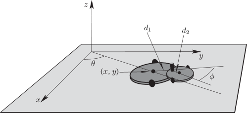
Figure 1: Roller Racer (taken from Bloch (2003) with permission from the author). The mass of the second body is assumed to be negligible.

The constraints are given by

$$\dot{x}=\cos\theta\csc\phi\left[(d_{1}\cos\phi+d_{2})\dot{\theta}+d_{2}\dot{\phi}\right],\qquad\dot{y}=\sin\theta\csc\phi\left[(d_{1}\cos\phi+d_{2})\dot{\theta}+d_{2}\dot{\phi}\right].$$ (III.3)

Defining the constraint one-forms

$$\omega^{1}\mathrel{\mathop{:}}=dx-\cos\theta\csc\phi[(d_{1}\cos\phi+d_{2})d\theta+d_{2}\,d\phi],\qquad\omega^{2}\mathrel{\mathop{:}}=dy-\sin\theta\csc\phi[(d_{1}\cos\phi+d_{2})d\theta+d_{2}\,d\phi],$$ (III.4)

we can write the constraint distribution $\Delta_{Q}\subset TQ$ as

$$\Delta_{Q}=\left\{\dot{q}=(\dot{x},\dot{y},\dot{\theta},\dot{\phi})\in TQ\ |\ \omega^{a}(\dot{q})=0,\,a=1,2\right\}.$$

The Lagrange–Dirac equations (II.3) give

$$\begin{array}[]{c}\displaystyle p_{x}=m_{1}v_{x},\qquad p_{y}=m_{1}v_{y},\qquad p_{\theta}=I_{1}v_{\theta},\qquad p_{\phi}=0,\vskip 6.0pt plus 2.0pt minus 2.0pt\\ \displaystyle\dot{x}=\cos\theta\csc\phi\left[(d_{1}\cos\phi+d_{2})\dot{\theta}+d_{2}\dot{\phi}\right],\qquad\dot{y}=\sin\theta\csc\phi\left[(d_{1}\cos\phi+d_{2})\dot{\theta}+d_{2}\dot{\phi}\right],\vskip 6.0pt plus 2.0pt minus 2.0pt\\ \displaystyle\dot{x}=v_{x},\qquad\dot{y}=v_{y},\qquad\dot{\theta}=v_{\theta},\qquad\dot{\phi}=v_{\phi},\vskip 6.0pt plus 2.0pt minus 2.0pt\\ \displaystyle\dot{p}_{x}=\lambda\sin\theta,\qquad\dot{p}_{y}=-\lambda\cos\theta,\qquad\dot{p}_{\theta}=0,\qquad\dot{p}_{\phi}=0,\end{array}$$ (III.5)

where $\lambda$ is the Lagrange multiplier.

Let $G=\mathbb{R}^{2}$ and consider the action of $G$ on $Q$ by translations on the $x$-$y$ plane, i.e.,

$$G\times Q\to Q;\quad\left((a,b),(x,y,\theta,\phi)\right)\mapsto(x+a,y+b,\theta,\phi).$$

Then, the tangent space to the group orbit is given by

$$T_{q}\mathcal{O}(q)=\operatorname{span}\left\{\dfrac{\partial}{\partial x},\dfrac{\partial}{\partial y}\right\},$$

with $q=(x,y,\theta,\phi)$. It is easy to check that this defines a Chaplygin system in the sense of Definition III.1. The quotient space is $\bar{Q}\mathrel{\mathop{:}}=Q/G=\{(\theta,\phi)\}$, and the horizontal lift $\operatorname{hl}^{\Delta}$ is

$$\operatorname{hl}^{\Delta}_{q}(\dot{\theta},\dot{\phi})=\left(\cos\theta\csc\phi\left[(d_{1}\cos\phi+d_{2})\dot{\theta}+d_{2}\dot{\phi}\right],\sin\theta\csc\phi\left[(d_{1}\cos\phi+d_{2})\dot{\theta}+d_{2}\dot{\phi}\right],\dot{\theta},\dot{\phi}\right).$$

Hence, the reduced Lagrangian $\bar{L}:T\bar{Q}\to\mathbb{R}$ is given by

$$\bar{L}=\frac{1}{2}m_{1}\left(d_{1}\dot{\theta}\cos\phi+d_{2}(\dot{\theta}+\dot{\phi})\right)^{2}\csc^{2}\phi+\frac{1}{2}I_{1}\dot{\theta}^{2},$$ (III.6)

which is non-degenerate; hence the simplified roller racer is a weakly degenerate Chaplygin system.

Therefore, the dynamics of the variables $\theta$ and $\phi$ are specified by the equations of motion, which together with the (nonholonomic) constraints, Eq. (III.3), determine the time evolution of the variables $x$ and $y$.

Example III.6 (Bicycle; see Getz (1994), Getz and Marsden (1995), and Koon and Marsden (1997)).

Consider the simplified model of a bicycle shown in Fig. 2: For the sake of simplicity, the wheels are assumed to be massless, and the mass $m$ of the bicycle is considered to be concentrated at a single point; however we take into account the moment of inertia of the steering wheel.

The configuration space is $Q=SE(2)\times\mathbb{S}^{1}\times\mathbb{S}^{1}=\{(x,y,\theta,\phi,\psi)\}$; the variables $x$, $y$, $\theta$, and $\psi$ are defined as in Fig. 2 and $\phi\mathrel{\mathop{:}}=\tan\sigma/b$; also let $J(\phi,\psi)$ be the moment of inertia associated with the steering action. The Lagrangian $L:TQ\to\mathbb{R}$ is given by

$$L=\frac{m}{2}\left[(\cos\theta\,\dot{x}+\sin\theta\,\dot{y}+a\sin\psi\,\dot{\theta})^{2}+(\sin\theta\,\dot{x}-\cos\theta\,\dot{y}+a\cos\psi\,\dot{\psi}-c\,\dot{\theta})^{2}\right.\\ \left.+a^{2}\sin\psi\,\dot{\psi}^{2}\right]+\frac{J(\phi,\psi)}{2}\,\dot{\phi}^{2}-mga\cos\psi,$$

which is degenerate.

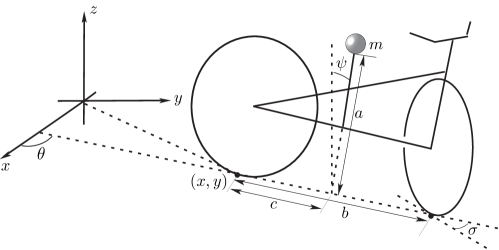
Figure 2: Bicycle (taken from Koon and Marsden (1997) with permission from Wang Sang Koon).

The constraints are given by

$$\dot{\theta}=\phi(\cos\theta\,\dot{x}+\sin\theta\,\dot{y}),\qquad\sin\theta\,\dot{x}-\cos\theta\,\dot{y}=0.$$

Defining the constraint one-forms

$$\omega^{1}\mathrel{\mathop{:}}=\phi(\cos\theta\,dx+\sin\theta\,dy),\qquad\omega^{2}\mathrel{\mathop{:}}=\sin\theta\,dx-\cos\theta\,dy,$$

we can write the constraint distribution $\Delta_{Q}\subset TQ$ as

$$\Delta_{Q}=\left\{\dot{q}=(\dot{x},\dot{y},\dot{\theta},\dot{\phi},\dot{\psi})\in TQ\ |\ \omega^{a}(\dot{q})=0,\,a=1,2\right\}.$$

Let $G=\mathbb{R}^{2}$ and consider the action of $G$ on $Q$ by translations on the $x$-$y$ plane, i.e.,

$$G\times Q\to Q;\quad\left((a,b),(x,y,\theta,\phi,\psi)\right)\mapsto(x+a,y+b,\theta,\phi,\psi).$$

Then, the tangent space to the group orbit is given by

$$T_{q}\mathcal{O}(q)=\operatorname{span}\left\{\dfrac{\partial}{\partial x},\dfrac{\partial}{\partial y}\right\},$$

with $q=(x,y,\theta,\phi,\psi)$. It is easy to check that this defines a Chaplygin system in the sense of Definition III.1. The quotient space is $\bar{Q}\mathrel{\mathop{:}}=Q/G=\{(\theta,\phi,\psi)\}$, and the horizontal lift $\operatorname{hl}^{\Delta}$ is

$$\operatorname{hl}^{\Delta}_{q}(\dot{\theta},\dot{\phi},\dot{\psi})=\left(\frac{\dot{\theta}}{\phi}\,\cos\theta,\frac{\dot{\theta}}{\phi}\,\sin\theta,\dot{\theta},\dot{\phi},\dot{\psi}\right).$$

Hence, the reduced Lagrangian $\bar{L}:T\bar{Q}\to\mathbb{R}$ is given by

$$\bar{L}=\frac{m}{2}\left[(c\,\dot{\theta}-a\cos\psi\,\dot{\psi})^{2}+\frac{(\dot{\theta}+a\sin\psi\,\dot{\theta})^{2}}{\phi^{2}}+a^{2}\sin\psi\,\dot{\psi}^{2}\right]+\frac{J(\phi,\psi)}{2}\,\dot{\phi}^{2}-mga\cos\psi,$$

which is non-degenerate, and so this is a weakly degenerate Chaplygin system as well.

IV Hamilton–Jacobi Theory for Lagrange–Dirac systems

IV.1 Hamilton–Jacobi Theorem for Lagrange–Dirac systems

We now state the main theorem of this paper, which relates the dynamics of the Lagrange–Dirac system with what we refer to as the Dirac–Hamilton–Jacobi equation.

Theorem IV.1 (Dirac–Hamilton–Jacobi Theorem).

Suppose that a Lagrangian $L:TQ\to\mathbb{R}$ and a distribution $\Delta_{Q}\subset TQ$ are given. Define $\Upsilon:Q\to TQ\oplus T^{*}Q$ by

$$\Upsilon(q)\mathrel{\mathop{:}}=\mathcal{X}(q)\oplus\gamma(q),$$

with a vector field $\mathcal{X}:Q\to TQ$ and a one-form $\gamma:Q\to T^{*}Q$, and assume that it satisfies

$$\Upsilon(q)\in\mathcal{K}_{q}\text{ for any }q\in Q,$$ (IV.1)

and

$$d\gamma|_{\Delta_{Q}}=0,\ \text{i.e.,}\ d\gamma(v,w)=0\text{ for any }v,w\in\Delta_{Q}.$$ (IV.2)

Then, the following are equivalent:

1. For every integral curve $c(t)$ of $\mathcal{X}$, i.e., for every curve $c:\mathbb{R}\to Q$ satisfying

   $$\dot{c}(t)=\mathcal{X}(c(t)),$$ (IV.3)

   the curve $t\mapsto\Upsilon\makebox[7.0pt]{\raisebox{1.0pt}{\tiny$\circ$}}c(t)=(\mathcal{X}\oplus\gamma)\makebox[7.0pt]{\raisebox{1.0pt}{\tiny$\circ$}}c(t)$ is an integral curve of the Lagrange–Dirac equations (II.3).

2. $\Upsilon$ satisfies the following Dirac–Hamilton–Jacobi equation:

   $$d(\mathcal{E}\makebox[7.0pt]{\raisebox{1.0pt}{\tiny$\circ$}}\Upsilon)\in\Delta_{Q}^{\circ},$$ (IV.4)

   or, if $Q$ is connected and $\Delta_{Q}$ is completely nonholonomic,

   $$\mathcal{E}\makebox[7.0pt]{\raisebox{1.0pt}{\tiny$\circ$}}\Upsilon=E,$$ (IV.5)

   with a constant $E$.

Proof.

Let us first show that (ii) implies (i). Assume (ii) and let $c(t)$ be an integral curve of $\mathcal{X}$, and then set

$$v(t)\oplus p(t)\mathrel{\mathop{:}}=\Upsilon\makebox[7.0pt]{\raisebox{1.0pt}{\tiny$\circ$}}c(t)=(\mathcal{X}\oplus\gamma)\makebox[7.0pt]{\raisebox{1.0pt}{\tiny$\circ$}}c(t).$$

Then, clearly $v(t)=\dot{c}(t)=\mathcal{X}(c(t))$. Also, Eq. (IV.1) implies that

$$v(t)\in\Delta_{Q}(c(t)),\quad p(t)=\dfrac{\partial L}{\partial v}(q(t),v(t)).$$

So it remains to show $\dot{p}-\partial L/\partial q\in\Delta_{Q}^{\circ}$. To that end, first calculate

$$\dot{p}_{j}(t)=\dfrac{d}{dt}\gamma_{j}\makebox[7.0pt]{\raisebox{1.0pt}{\tiny$\circ$}}c(t)=\dfrac{\partial\gamma_{j}}{\partial q^{i}}(c(t))\,\dot{c}^{i}(t)=\dfrac{\partial\gamma_{j}}{\partial q^{i}}(c(t))\,\mathcal{X}^{i}(c(t))$$

and so, for any $w\in\Delta_{Q}$, we have

$$\dot{p}_{j}(t)w^{j}=\dfrac{\partial\gamma_{j}}{\partial q^{i}}(c(t))\,\mathcal{X}^{i}(c(t))\,w^{j}=\dfrac{\partial\gamma_{i}}{\partial q^{j}}(c(t))\,\mathcal{X}^{i}(c(t))\,w^{j},$$ (IV.6)

since Eq. (IV.2) implies, for any $v,w\in\Delta_{Q}$,

$$\dfrac{\partial\gamma_{i}}{\partial q^{j}}v^{i}w^{j}=\dfrac{\partial\gamma_{j}}{\partial q^{i}}v^{i}w^{j},$$

and also Eq. (IV.1) gives $\mathcal{X}(q)\in\Delta_{Q}(q)$. On the other hand,

$$d(\mathcal{E}\makebox[7.0pt]{\raisebox{1.0pt}{\tiny$\circ$}}\Upsilon) =d(\gamma_{i}(q)\,\mathcal{X}^{i}(q)-L(q,\mathcal{X}(q)))$$

$$=\left(\dfrac{\partial\gamma_{i}}{\partial q^{j}}\mathcal{X}^{i}+\gamma_{i}\dfrac{\partial\mathcal{X}^{i}}{\partial q^{j}}-\dfrac{\partial L}{\partial q^{j}}-\dfrac{\partial L}{\partial v^{i}}\dfrac{\partial\mathcal{X}^{i}}{\partial q^{j}}\right)dq^{j}$$

$$=\left(\dfrac{\partial\gamma_{i}}{\partial q^{j}}\mathcal{X}^{i}-\dfrac{\partial L}{\partial q^{j}}\right)dq^{j},$$

where we used the following relation that follows from Eq. (IV.1):

$$\gamma(q)=\dfrac{\partial L}{\partial v}(q,\mathcal{X}(q)).$$

So the Dirac–Hamilton–Jacobi equation (IV.4) with Eq. (IV.6) implies

$$d(\mathcal{E}\makebox[7.0pt]{\raisebox{1.0pt}{\tiny$\circ$}}\Upsilon)(c(t))\cdot w =\left(\dfrac{\partial\gamma_{i}}{\partial q^{j}}(c(t))\,\mathcal{X}^{i}(c(t))-\dfrac{\partial L}{\partial q^{j}}(c(t),v(t))\right)w^{j}$$

$$=\left(\dot{p}_{j}(t)-\dfrac{\partial L}{\partial q^{j}}(c(t),v(t))\right)w^{j}=0.$$

Since $w\in\Delta_{Q}$ is arbitrary, this implies

$$\dot{p}(t)-\dfrac{\partial L}{\partial q}(c(t),v(t))\in\Delta_{Q}^{\circ}.$$

Therefore, (i) is satisfied.

Conversely, assume (i); let $c(t)$ be a curve in $Q$ that satisfies Eq. (IV.3) and set $v(t)\oplus p(t)\mathrel{\mathop{:}}=\Upsilon\makebox[7.0pt]{\raisebox{1.0pt}{\tiny$\circ$}}c(t)=(\mathcal{X}\oplus\gamma)\makebox[7.0pt]{\raisebox{1.0pt}{\tiny$\circ$}}c(t)$. Then, by assumption, $(c(t),v(t),p(t))$ is an integral curve of the Lagrange–Dirac system (II.2), and so

$$\dot{p}(t)-\dfrac{\partial L}{\partial q}(c(t),v(t))\in\Delta_{Q}^{\circ}(c(t)).$$

Following the same calculations as above we have, for any $w\in\Delta_{Q}$,

$$d(\mathcal{E}\makebox[7.0pt]{\raisebox{1.0pt}{\tiny$\circ$}}\Upsilon)(c(t))\cdot w=\left(\dot{p}_{j}(t)-\dfrac{\partial L}{\partial q^{j}}(c(t),v(t))\right)w^{j}=0.$$

For an arbitrary point $q\in Q$, we can consider an integral curve $c(t)$ of $X$ such that $c(0)=q$. Therefore, the above equation implies that $d(\mathcal{E}\makebox[7.0pt]{\raisebox{1.0pt}{\tiny$\circ$}}\Upsilon)(q)\cdot w_{q}=0$ for any $q\in Q$ and $w_{q}\in\Delta_{Q}(q)$, which gives the Dirac–Hamilton–Jacobi equation (IV.4). If $Q$ is connected and $\Delta_{Q}$ is completely nonholonomic, then by the same argument as in the proof of Theorem 3.1 in Ohsawa and Bloch (2009), $d(\mathcal{E}\makebox[7.0pt]{\raisebox{1.0pt}{\tiny$\circ$}}\Upsilon)\in\Delta_{Q}^{\circ}$ reduces to $\mathcal{E}\makebox[7.0pt]{\raisebox{1.0pt}{\tiny$\circ$}}\Upsilon=E$ for some constant $E$. ∎

Theorem IV.1 can be recast in the context of Section II.4 as follows:

Corollary IV.2.

Under the same conditions as in Theorem IV.1, the following are equivalent:

1. For every curve $c(t)$ such that

   $$\dot{c}(t)=T\mathrm{pr}_{Q}\cdot\tilde{X}(\Upsilon\makebox[7.0pt]{\raisebox{1.0pt}{\tiny$\circ$}}c(t)),$$

   the curve $t\mapsto\Upsilon\makebox[7.0pt]{\raisebox{1.0pt}{\tiny$\circ$}}c(t)$ is an integral curve of $\tilde{X}$, and so it is an integral curve of the Lagrange–Dirac equations (II.3).

2. $\Upsilon$ satisfies $(0,d(\mathcal{E}\makebox[7.0pt]{\raisebox{1.0pt}{\tiny$\circ$}}\Upsilon\makebox[7.0pt]{\raisebox{1.0pt}{\tiny$\circ$}}\mathrm{pr}_{Q}))\in D_{TQ\oplus T^{*}Q}$, or equivalently, $d(\mathcal{E}\makebox[7.0pt]{\raisebox{1.0pt}{\tiny$\circ$}}\Upsilon\makebox[7.0pt]{\raisebox{1.0pt}{\tiny$\circ$}}\mathrm{pr}_{Q})\in\Delta_{TQ\oplus T^{*}Q}^{\circ}$.

Proof.

The equivalence of (i) with that of Theorem IV.1 follows from the relation $T\mathrm{pr}_{Q}\makebox[7.0pt]{\raisebox{1.0pt}{\tiny$\circ$}}\tilde{X}\makebox[7.0pt]{\raisebox{1.0pt}{\tiny$\circ$}}\Upsilon=\mathcal{X}$, which is easily checked by coordinate calculations.

On the other hand, for (ii), first observe that $\mathrm{pr}_{Q}^{*}(\Delta_{Q}^{\circ})=\Delta_{TQ\oplus T^{*}Q}^{\circ}$. Then, since $\mathrm{pr}_{Q}:TQ\oplus T^{*}Q\to Q$ is a surjective submersion, it follows that

$$d(\mathcal{E}\makebox[7.0pt]{\raisebox{1.0pt}{\tiny$\circ$}}\Upsilon)\in\Delta_{Q}^{\circ}\iff\mathrm{pr}_{Q}^{*}d(\mathcal{E}\makebox[7.0pt]{\raisebox{1.0pt}{\tiny$\circ$}}\Upsilon)\in\mathrm{pr}_{Q}^{*}(\Delta_{Q}^{\circ})\iff d(\mathcal{E}\makebox[7.0pt]{\raisebox{1.0pt}{\tiny$\circ$}}\Upsilon\makebox[7.0pt]{\raisebox{1.0pt}{\tiny$\circ$}}\mathrm{pr}_{Q})\in\Delta_{TQ\oplus T^{*}Q}^{\circ}.$$

This proves the equivalence of (ii) with that of Theorem IV.1. ∎

IV.2 Nonholonomic Hamilton–Jacobi Theory as a Special Case

Let us show that the nonholonomic Hamilton–Jacobi equation of Iglesias-Ponte et al. (2008) and Ohsawa and Bloch (2009) follows as a special case of the above theorem. Consider the special case where the Lagrangian $L:TQ\to\mathbb{R}$ is non-degenerate, i.e., the Legendre transformation $\mathbb{F}L:TQ\to T^{*}Q$ is invertible. Then, we may rewrite the definition of the submanifold $\mathcal{K}\subset TQ\oplus T^{*}Q$, Eq. (II.4), by

$$\mathcal{K} =\left\{v_{q}\oplus p_{q}\in TQ\oplus T^{*}Q\ |\ v_{q}\in\Delta_{Q}(q),\ p_{q}=\mathbb{F}L(v_{q})\right\}$$

$$=\left\{v_{q}\oplus p_{q}\in TQ\oplus T^{*}Q\ |\ p_{q}\in P_{q},\ v_{q}=(\mathbb{F}L)^{-1}(p_{q})\right\}$$

$$=\Delta_{Q}\oplus P,$$

where we recall that $P\mathrel{\mathop{:}}=\mathbb{F}L(\Delta_{Q})$. It implies that if $\Upsilon=\mathcal{X}\oplus\gamma$ takes values in $\mathcal{K}$ then $\mathcal{X}=(\mathbb{F}L)^{-1}\makebox[7.0pt]{\raisebox{1.0pt}{\tiny$\circ$}}\gamma$, and thus

$$\mathcal{E}\makebox[7.0pt]{\raisebox{1.0pt}{\tiny$\circ$}}\Upsilon(q)=\left\langle\gamma(q),(\mathbb{F}L)^{-1}(\gamma(q))\right\rangle-L\makebox[7.0pt]{\raisebox{1.0pt}{\tiny$\circ$}}(\mathbb{F}L)^{-1}(\gamma(q))=H\makebox[7.0pt]{\raisebox{1.0pt}{\tiny$\circ$}}\gamma(q),$$

with $\gamma$ taking values in $P$ and the Hamiltonian $H:T^{*}Q\to\mathbb{R}$ defined by

$$H(q,p)\mathrel{\mathop{:}}=\left\langle p_{q},(\mathbb{F}L)^{-1}(p_{q})\right\rangle-L\makebox[7.0pt]{\raisebox{1.0pt}{\tiny$\circ$}}(\mathbb{F}L)^{-1}(p_{q}).$$

Then, the Lagrange–Dirac equations (II.3) become the nonholonomic Hamilton’s equations

$$\dot{q}=\frac{\partial H}{\partial p}(q,p),\qquad\dot{p}+\frac{\partial H}{\partial q}(q,p)\in\Delta_{Q}^{\circ}(q).\qquad\dot{q}\in\Delta_{Q}(q),$$

or, in an intrinsic form,

$$i_{X_{H}^{\rm nh}}\Omega-dH\in\Delta_{T^{*}Q}^{\circ},\qquad T\pi_{Q}(X_{H}^{\rm nh})\in\Delta_{Q}$$

for a vector field $X_{H}^{\rm nh}$ on $T^{*}Q$. Furthermore, it is straightforward to show that

$$(\mathbb{F}L)^{-1}=\mathbb{F}H=T\pi_{Q}\makebox[7.0pt]{\raisebox{1.0pt}{\tiny$\circ$}}X_{H},$$

where $X_{H}$ is the Hamiltonian vector field of the unconstrained system with the same Hamiltonian, i.e., $i_{X_{H}}\Omega=dH$; hence we obtain

$$\mathcal{X}(q)=(\mathbb{F}L)^{-1}\makebox[7.0pt]{\raisebox{1.0pt}{\tiny$\circ$}}\gamma(q)=T\pi_{Q}\cdot X_{H}(\gamma(q)).$$

Therefore, Theorem IV.1 specializes to the nonholonomic Hamilton–Jacobi theorem of Iglesias-Ponte et al. (2008) and Ohsawa and Bloch (2009):

Corollary IV.3 (Nonholonomic Hamilton–Jacobi Iglesias-Ponte et al. (2008); Ohsawa and Bloch (2009)).

Consider a nonholonomic system defined on a configuration manifold $Q$ with a Lagrangian of the form Eq. (III.2) and a nonholonomic constraint distribution $\Delta_{Q}\subset TQ$. Let $\gamma:Q\to T^{*}Q$ be a one-form that satisfies

$$\gamma(q)\in P_{q}\text{ for any }q\in Q,$$

and

$$d\gamma|_{\Delta_{Q}}=0,\text{ i.e., }d\gamma(v,w)=0\text{ for any }v,w\in\Delta_{Q}.$$

Then, the following are equivalent:

1. For every curve $c(t)$ in $Q$ satisfying

   $$\dot{c}(t)=T\pi_{Q}\cdot X_{H}(\gamma\makebox[7.0pt]{\raisebox{1.0pt}{\tiny$\circ$}}c(t)),$$

   the curve $t\mapsto\gamma\makebox[7.0pt]{\raisebox{1.0pt}{\tiny$\circ$}}c(t)$ is an integral curve of $X_{H}^{\rm nh}$, where $X_{H}$ is the Hamiltonian vector field of the unconstrained system with the same Hamiltonian, i.e., $i_{X_{H}}\Omega=dH$.

2. The one-form $\gamma$ satisfies the nonholonomic Hamilton–Jacobi equation:

   $$d(H\makebox[7.0pt]{\raisebox{1.0pt}{\tiny$\circ$}}\gamma)\in\Delta_{Q}^{\circ},$$

   or, if $Q$ is connected and $\Delta_{Q}$ is completely nonholonomic,

   $$H\makebox[7.0pt]{\raisebox{1.0pt}{\tiny$\circ$}}\gamma=E,$$

   with a constant $E$.

IV.3 Applications to Degenerate Lagrangian System with Holonomic Constraints

If the constraints are holonomic, then the distribution $\Delta_{Q}\subset TQ$ is integrable, and so there exists a local submanifold $S\subset Q$ such that $T_{s}S=\Delta_{Q}(s)$ for any $s\in S$. Let $\iota_{S}:S\hookrightarrow Q$ be the inclusion. Then, the Dirac–Hamilton–Jacobi equation (IV.4) gives

$$\iota_{S}^{*}d(\mathcal{E}\makebox[7.0pt]{\raisebox{1.0pt}{\tiny$\circ$}}\Upsilon)\in(TS)^{\circ}=0,$$

and thus

$$d(\mathcal{E}\makebox[7.0pt]{\raisebox{1.0pt}{\tiny$\circ$}}\Upsilon\makebox[7.0pt]{\raisebox{1.0pt}{\tiny$\circ$}}\iota_{S})=0,$$

which implies that we have

$$\mathcal{E}\makebox[7.0pt]{\raisebox{1.0pt}{\tiny$\circ$}}\Upsilon\makebox[7.0pt]{\raisebox{1.0pt}{\tiny$\circ$}}\iota_{S}=E,$$ (IV.7)

with a constant $E$, assuming $S$ is connected.

On the other hand, the condition (IV.2) becomes

$$\iota_{S}^{*}d\gamma=d(\gamma\makebox[7.0pt]{\raisebox{1.0pt}{\tiny$\circ$}}\iota_{S})=0,$$ (IV.8)

and so $\gamma\makebox[7.0pt]{\raisebox{1.0pt}{\tiny$\circ$}}\iota_{S}=dW$ for some function $W$ defined locally on $S$.

Example IV.4 (LC circuit; see Yoshimura and Marsden (2006a, 2007)).

Consider the LC circuit shown in Fig. 3.

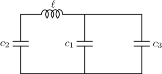
Figure 3: LC circuit (see Yoshimura and Marsden (2006a)).

The configuration space is the 4-dimensional vector space $Q=\{(q_{\ell},q_{c_{1}},q_{c_{2}},q_{c_{3}})\}$, which represents charges in the circuit elements. Then $TQ\cong Q\times Q$ and $f_{q}=(f_{\ell},f_{c_{1}},f_{c_{2}},f_{c_{3}})\in T_{q}Q$ represents the currents in the corresponding circuit elements. The Lagrangian $L:TQ\to\mathbb{R}$ is given by

$$L(q,f)=\frac{1}{2}\ell\,f_{\ell}^{2}-\frac{1}{2}\frac{q_{c_{1}}^{2}}{c_{1}}-\frac{1}{2}\frac{q_{c_{2}}^{2}}{c_{2}}-\frac{1}{2}\frac{q_{c_{3}}^{2}}{c_{3}},$$

which is clearly degenerate.

The generalized energy $\mathcal{E}:TQ\oplus T^{*}Q\to\mathbb{R}$ is

$$\mathcal{E}(q,f,p) =p\cdot f-L(q,f)$$

$$=p_{\ell}f_{\ell}+p_{c_{1}}f_{c_{1}}+p_{c_{2}}f_{c_{2}}+p_{c_{3}}f_{c_{3}}-\frac{1}{2}\ell\,f_{\ell}^{2}+\frac{1}{2}\frac{q_{c_{1}}^{2}}{c_{1}}+\frac{1}{2}\frac{q_{c_{2}}^{2}}{c_{2}}+\frac{1}{2}\frac{q_{c_{3}}^{2}}{c_{3}}.$$

The Kirchhoff current law gives the constraints $-f_{\ell}+f_{c_{2}}=0$ and $f_{c_{1}}-f_{c_{2}}+f_{c_{3}}=0$, or in terms of constraint one-forms, $\omega^{1}=-dq_{\ell}+dq_{c_{2}}$ and $\omega^{2}=dq_{c_{1}}-dq_{c_{2}}+dq_{c_{3}}$. Thus, the constraint distribution $\Delta_{Q}\subset TQ$ is given by

$$\Delta_{Q}=\left\{f\in TQ\ |\ \omega^{a}(f)=0,\,a=1,2\right\}.$$

So the submanifold $\mathcal{K}\subset TQ\oplus T^{*}Q$ is

$$\mathcal{K}=\left\{(q,f,p)\in TQ\oplus T^{*}Q\ |\ f_{\ell}=f_{c_{2}},\ f_{c_{2}}=f_{c_{1}}+f_{c_{3}},\ p_{\ell}=\ell\,f_{\ell},\ p_{c_{1}}=p_{c_{2}}=p_{c_{3}}=0\right\}.$$

Hence, the generalized energy constrained to $\mathcal{K}$ is

$$\mathcal{E}|_{\mathcal{K}}=\frac{1}{2}\ell\,f_{\ell}^{2}+\frac{1}{2}\frac{q_{c_{1}}^{2}}{c_{1}}+\frac{1}{2}\frac{q_{c_{2}}^{2}}{c_{2}}+\frac{1}{2}\frac{q_{c_{3}}^{2}}{c_{3}}.$$

Notice that the constraints are holonomic, i.e., the constraints can be integrated to give

$$q_{\ell}-q_{c_{2}}=a_{0},\quad q_{c_{2}}-q_{c_{1}}-q_{c_{3}}=a_{1},$$

with some constants $a_{0}$ and $a_{1}$. So we define a submanifold $S\subset Q$ by

$$S\mathrel{\mathop{:}}=\left\{(q_{\ell},q_{c_{1}},q_{c_{2}},q_{c_{3}})\in Q\ |\ q_{c_{2}}=q_{\ell}-a_{0},\;q_{c_{3}}=q_{c_{2}}-q_{c_{1}}-a_{1}\right\}=\{(q_{\ell},q_{c_{1}})\},$$

and the inclusion

$$\iota_{S}:S\hookrightarrow Q;\quad(q_{\ell},q_{c_{1}})\mapsto(q_{\ell},q_{c_{1}},q_{\ell}-a_{0},q_{c_{2}}-q_{c_{1}}-a_{1}).$$

Now, the Dirac–Hamilton–Jacobi equation for holonomic systems, Eq. (IV.7), gives

$$\mathcal{E}\makebox[7.0pt]{\raisebox{1.0pt}{\tiny$\circ$}}\Upsilon\makebox[7.0pt]{\raisebox{1.0pt}{\tiny$\circ$}}\iota_{S}=E,$$ (IV.9)

with some constant $E$, where $\Upsilon\makebox[7.0pt]{\raisebox{1.0pt}{\tiny$\circ$}}\iota_{S}:S\to TQ\oplus T^{*}Q$ is

$$\Upsilon\makebox[7.0pt]{\raisebox{1.0pt}{\tiny$\circ$}}\iota_{S}(q_{\ell},q_{c_{1}})=\left(q_{\ell},q_{c_{1}},\tilde{\mathcal{X}}(q_{\ell},q_{c_{1}}),\tilde{\gamma}(q_{\ell},q_{c_{1}})\right)$$

with $\tilde{\mathcal{X}}\mathrel{\mathop{:}}=\mathcal{X}\makebox[7.0pt]{\raisebox{1.0pt}{\tiny$\circ$}}\iota_{S}:S\to TQ$ and $\tilde{\gamma}\mathrel{\mathop{:}}=\gamma\makebox[7.0pt]{\raisebox{1.0pt}{\tiny$\circ$}}\iota_{S}:S\to T^{*}Q$ given by

$$\tilde{\mathcal{X}}(q_{\ell},q_{c_{1}}) =\left(\tilde{\mathcal{X}}_{\ell}(q_{\ell},q_{c_{1}}),\tilde{\mathcal{X}}_{c_{1}}(q_{\ell},q_{c_{1}}),\tilde{\mathcal{X}}_{c_{2}}(q_{\ell},q_{c_{1}}),\tilde{\mathcal{X}}_{c_{3}}(q_{\ell},q_{c_{1}})\right),$$

$$\tilde{\gamma}(q_{\ell},q_{c_{1}}) =\left(\tilde{\gamma}_{\ell}(q_{\ell},q_{c_{1}}),\tilde{\gamma}_{c_{1}}(q_{\ell},q_{c_{1}}),\tilde{\gamma}_{c_{2}}(q_{\ell},q_{c_{1}}),\tilde{\gamma}_{c_{3}}(q_{\ell},q_{c_{1}})\right).$$

The condition $\Upsilon\makebox[7.0pt]{\raisebox{1.0pt}{\tiny$\circ$}}\iota_{S}(q_{\ell},q_{c_{1}})\in\mathcal{K}$ implies

$$\tilde{\mathcal{X}}_{\ell}=\tilde{\mathcal{X}}_{c_{2}},\quad\tilde{\mathcal{X}}_{c_{2}}=\tilde{\mathcal{X}}_{c_{1}}+\tilde{\mathcal{X}}_{c_{3}},\quad\tilde{\gamma}_{\ell}=\ell\,\tilde{\mathcal{X}}_{\ell},\quad\tilde{\gamma}_{c_{1}}=\tilde{\gamma}_{c_{2}}=\tilde{\gamma}_{c_{3}}=0.$$

Then,

$$\tilde{\gamma}=\gamma\makebox[7.0pt]{\raisebox{1.0pt}{\tiny$\circ$}}\iota_{S}=\ell\,\tilde{\mathcal{X}}_{\ell}(q_{\ell},q_{c_{1}})\,dq_{\ell},$$

and thus condition (IV.8) gives

$$\dfrac{\partial\tilde{\mathcal{X}}_{\ell}}{\partial q_{c_{1}}}=0,$$

and hence $\tilde{\mathcal{X}}_{\ell}(q_{\ell},q_{c_{1}})=\tilde{\mathcal{X}}_{\ell}(q_{\ell})$. The Dirac–Hamilton–Jacobi equation (IV.9) then becomes

$$\frac{1}{2}\ell\,\tilde{\mathcal{X}}_{\ell}(q_{\ell})^{2}+\frac{1}{2}\frac{q_{c_{1}}^{2}}{c_{1}}+\frac{1}{2}\frac{(q_{\ell}-a_{0})^{2}}{c_{2}}+\frac{1}{2}\frac{(q_{\ell}-q_{c_{1}}-a_{0}-a_{1})^{2}}{c_{3}}=E.$$ (IV.10)

We impose the condition that $\mathcal{X}_{\ell}=0$ when $q_{\ell}=q_{c_{1}}=0$ and $E=0$, which corresponds to the case where nothing is happening in the circuit. Then, we have

$$\frac{a_{0}^{2}}{c_{2}}+\frac{(a_{0}+a_{1})^{2}}{c_{3}}=0,$$

which gives $a_{0}=a_{1}=0$, since $c_{2}$ and $c_{3}$ are both positive. Therefore, Eq. (IV.10) becomes

$$\frac{1}{2}\ell\,\tilde{\mathcal{X}}_{\ell}(q_{\ell})^{2}+\frac{1}{2}\frac{q_{c_{1}}^{2}}{c_{1}}+\frac{1}{2}\frac{q_{\ell}^{2}}{c_{2}}+\frac{1}{2}\frac{(q_{\ell}-q_{c_{1}})^{2}}{c_{3}}=E.$$ (IV.11)

Taking the derivative with respect to $q_{c_{1}}$ of both sides and solving for $q_{c_{1}}$, we have

$$q_{c_{1}}=\frac{c_{1}}{c_{1}+c_{3}}\,q_{\ell}.$$

Substituting this into Eq. (IV.11) gives

$$\frac{1}{2}\left(\ell\,\tilde{\mathcal{X}}_{\ell}(q_{\ell})^{2}+\frac{c_{1}+c_{2}+c_{3}}{c_{2}(c_{1}+c_{3})}\,q_{\ell}^{2}\right)=E.$$

Solving for $\tilde{\mathcal{X}}_{\ell}(q_{\ell})$, we obtain

$$\mathcal{X}_{\ell}(q)=\tilde{\mathcal{X}}_{\ell}(q_{\ell})=\pm\sqrt{\frac{1}{\ell}\left(2E-\frac{c_{1}+c_{2}+c_{3}}{c_{2}(c_{1}+c_{3})}\,q_{\ell}^{2}\right)}.$$

Taking the positive root, Eq. (IV.3) for $q_{\ell}$ gives

$$\dot{q}_{\ell}=\sqrt{\frac{1}{\ell}\left(2E-\frac{c_{1}+c_{2}+c_{3}}{c_{2}(c_{1}+c_{3})}\,q_{\ell}^{2}\right)},$$

which can be solved easily:

$$q_{\ell}(t)=\sqrt{\frac{2E}{\ell\,\nu^{2}}}\,\sin(\nu t+\alpha),$$

where

$$\nu\mathrel{\mathop{:}}=\sqrt{\frac{c_{1}+c_{2}+c_{3}}{c_{2}(c_{1}+c_{3})\,\ell}}$$

and $\alpha$ is a phase constant to be determined by the initial condition.

Remark IV.5.

In the conventional LC circuit theory, one often simplifies problems by “combining” capacitors. Using this technique, the above example simplifies to an LC circuit with an inductor with inductance $\ell$ and a single capacitance $C$, that satisfies the following equation:

$$\frac{1}{C}=\frac{1}{c_{2}}+\frac{1}{c_{1}+c_{3}},$$

which gives

$$C=\frac{c_{2}(c_{1}+c_{3})}{c_{1}+c_{2}+c_{3}}.$$

Then, the equation for the current $i_{\ell}\mathrel{\mathop{:}}=\dot{q}_{\ell}$ is given by

$$\ell\,\dfrac{d^{2}{i}_{\ell}}{dt^{2}}+\frac{i_{\ell}}{C}=0,$$

or

$$\dfrac{d^{2}{i}_{\ell}}{dt^{2}}+\nu\,i_{\ell}=0,$$

with

$$\nu=\frac{1}{\sqrt{\ell\,C}}=\sqrt{\frac{c_{1}+c_{2}+c_{3}}{c_{2}(c_{1}+c_{3})\,\ell}},$$

which coincides the one defined above. The general solution of the above ODE is

$$i_{\ell}(t)=\dot{q}_{\ell}(t)=A\sin(\nu t+\alpha)$$

for some constants $A$ and $\alpha$. Therefore, our solution is consistent with the conventional theory.

IV.4 Applications to Degenerate Lagrangian System with Nonholonomic Constraints

Example IV.6 (Simplified Roller Racer; see Example III.5).

The submanifold $\mathcal{K}\subset TQ\oplus T^{*}Q$ is given by

$$\mathcal{K}=\Bigl{\{}(q,v,p)\in TQ\oplus T^{*}Q\ |\ v_{x}=\cos\theta\csc\phi[(d_{1}\cos\phi+d_{2})\,v_{\theta}+d_{2}v_{\phi}],\\ v_{y}=\sin\theta\csc\phi[(d_{1}\cos\phi+d_{2})\,v_{\theta}+d_{2}v_{\phi}],\;p_{x}=m_{1}v_{x},\;p_{y}=m_{1}v_{y},\;p_{\theta}=I_{1}v_{\theta},\;p_{\phi}=0\Bigr{\}},$$

and the generalized energy constrained to $\mathcal{K}$ is

$$\mathcal{E}|_{\mathcal{K}}=\frac{1}{2}m_{1}\csc^{2}\phi\left[(d_{1}\cos\phi+d_{2})\,v_{\theta}+d_{2}v_{\phi}\right]^{2}+\frac{1}{2}I_{1}v_{\theta}^{2}.$$

The distribution $\Delta_{Q}$ is easily shown to be completely nonholonomic, and thus we may use the Dirac–Hamilton–Jacobi equation (IV.5), which gives

$$\frac{1}{2}m_{1}\csc^{2}\phi\left[(d_{1}\cos\phi+d_{2})\,\mathcal{X}_{\theta}(q)+d_{2}\mathcal{X}_{\phi}(q)\right]^{2}+\frac{1}{2}I_{1}\mathcal{X}_{\theta}(q)^{2}=E.$$ (IV.12)

Now, we assume the following ansatz:

$$\mathcal{X}_{\theta}(x,y,\theta,\phi)=\mathcal{X}_{\theta}(\theta,\phi),\qquad\mathcal{X}_{\phi}(x,y,\theta,\phi)=\mathcal{X}_{\phi}(\phi).$$ (IV.13)

However, substituting them into Eq. (IV.12) and solving for $\mathcal{X}_{\theta}$ shows that $\mathcal{X}_{\theta}$ does not depend on $\theta$ either; hence we set $\mathcal{X}_{\theta}(\theta,\phi)=\mathcal{X}_{\theta}(\phi)$. Then, solving Eq. (IV.12) for $\mathcal{X}_{\phi}$, we have

$$\mathcal{X}_{\phi}(\phi)=\frac{-(d_{1}\cos\phi+d_{2})\mathcal{X}_{\theta}(\phi)\pm\sin\phi\sqrt{2E-I_{1}\mathcal{X}_{\theta}(\phi)^{2}}}{\sqrt{m_{1}}\,d_{2}}.$$ (IV.14)

Substituting the first solution into condition (IV.2), we have

$$\left[(d_{1}\cos\phi+d_{2})\,\mathcal{X}_{\theta}(\phi)-\sin\phi\sqrt{2E-I_{1}\mathcal{X}_{\theta}(\phi)^{2}}\right]\mathcal{X}_{\theta}^{\prime}(\phi)=0.$$

We choose $\mathcal{X}_{\theta}^{\prime}(\phi)=0$ and hence

$$\mathcal{X}_{\theta}(\phi)=v_{\theta},$$

where $v_{\theta}$ is the initial angular velocity in the $\theta$-direction. This is consistent with the Lagrange–Dirac equations (III.5), which give $\ddot{\theta}=0$. Substituting this into the first case of Eq. (IV.14), we obtain

$$\mathcal{X}_{\phi}(\phi)=-v_{\theta}\left(1+\frac{d_{1}}{d_{2}}\cos\phi\right)+\frac{v_{r}}{d_{2}}\sin\phi,$$

where $v_{r}\mathrel{\mathop{:}}=\sqrt{(2E-I_{1}v_{\theta}^{2})/m_{1}}$.

Then, the condition $\mathcal{X}(q)\in\Delta_{Q}(q)$ gives the other components of the vector field $\mathcal{X}$, and hence Eq. (IV.3) gives

$$\begin{array}[]{c}\dot{x}=v_{r}\cos\theta,\qquad\dot{y}=v_{r}\sin\theta,\vskip 12.0pt plus 4.0pt minus 4.0pt\\ \displaystyle\dot{\theta}=0,\qquad\displaystyle\dot{\phi}=-v_{\theta}\left(1+\frac{d_{1}}{d_{2}}\cos\phi\right)+\frac{v_{r}}{d_{2}}\sin\phi.\end{array}$$

We can solve the last equation by separation of variables, and the rest is explicitly solvable.

IV.5 Lagrangians that are Linear in Velocity

There are some physical systems, such as point vortices (see, e.g., Chapman (1978) and Newton (2001)), which are described by Lagrangians that are linear in velocity, i.e.,

$$L(q,\dot{q})=\left\langle\alpha(q),\dot{q}\right\rangle-h(q),$$ (IV.15)

where $\alpha$ is a one-form on $Q$. The Lagrangian is clearly degenerate and Lagrange–Dirac equations (II.3) give the following equations of motion (see Rowley and Marsden (2002) and Yoshimura and Marsden (2007)):

$$-i_{\mathcal{X}}d\alpha=dh,$$ (IV.16)

where $\mathcal{X}$ is a vector field on $Q$; hence the Lagrange–Dirac equations (II.3) reduce to the first-order dynamics $\dot{q}=\mathcal{X}(q)$ defined on $Q$.

Now, the assumption in (IV.1) of Theorem IV.1 implies $\gamma(q)=\alpha(q)$ and thus

$$\mathcal{E}\makebox[7.0pt]{\raisebox{1.0pt}{\tiny$\circ$}}\Upsilon(q)=h(q);$$

so the Dirac–Hamilton–Jacobi equation (IV.4) gives

$$h(q)=E,$$

which simply defines a level set of the energy of the dynamics on $Q$, i.e., the Dirac–Hamilton–Jacobi equation (IV.5) does not give any information on the dynamics on $Q$. This is because the original dynamics, which is naturally defined on $Q$ with the one-form $\alpha$ and the function $h$, is somewhat artificially lifted to the tangent bundle $TQ$ through the linear Lagrangian (IV.15). In fact, for point vortices on the plane, one has $Q=\mathbb{R}^{2}$, and the two-form $-d\alpha$ is a symplectic form; hence $Q=\mathbb{R}^{2}$ is a symplectic manifold and Eq. (IV.16) defines a Hamiltonian system on $Q$ with the Hamiltonian $h$.

V Hamilton–Jacobi Theory for Weakly Degenerate Chaplygin Systems

In this section, we first show that a weakly Chaplygin system introduced in Section III.2 reduces to an almost Hamiltonian system on $T^{*}\bar{Q}$ with a reduced Hamiltonian $\bar{H}:T^{*}\bar{Q}\to\mathbb{R}$, where $\bar{Q}\mathrel{\mathop{:}}=Q/G$. Accordingly, we may consider a variant of the nonholonomic Hamilton–Jacobi equation Iglesias-Ponte et al. (2008); Ohsawa and Bloch (2009) for the reduced system, which we call the reduced Dirac–Hamilton–Jacobi equation. We then show an explicit formula that maps solutions of the reduced Dirac–Hamilton–Jacobi equation to those of the original one. Thus, one may solve the reduced Dirac–Hamilton–Jacobi equation, which is simpler than the original one, and then construct solutions of the original Dirac–Hamilton–Jacobi equation by the formula.

V.1 The Geometry of Weakly Degenerate Chaplygin Systems

For weakly degenerate Chaplygin systems, the geometric structure introduced in Section III.1 is carried over to the Hamiltonian side. Specifically, we define the horizontal lift $\operatorname{hl}^{P}_{q}:T_{\bar{q}}^{*}\bar{Q}\to P_{q}$ by (see Ehlers et al. (2004))

$$\operatorname{hl}^{P}_{q}\mathrel{\mathop{:}}=\mathbb{F}L_{q}\makebox[7.0pt]{\raisebox{1.0pt}{\tiny$\circ$}}\operatorname{hl}^{\Delta}_{q}\makebox[7.0pt]{\raisebox{1.0pt}{\tiny$\circ$}}(\mathbb{F}\bar{L})^{-1}_{\bar{q}},$$

or by requiring that the diagram below commutes.

It is easy to show that the following equality holds for the pairing between the two horizontal lifts (see Lemma A.1 in Ohsawa et al. (2011)): For any $\alpha_{\bar{q}}\in T^{*}_{\bar{q}}\bar{Q}$ and $v_{\bar{q}}\in T_{\bar{q}}\bar{Q}$,

$$\left\langle\operatorname{hl}^{P}_{q}(\alpha_{\bar{q}}),\operatorname{hl}^{\Delta}_{q}(v_{\bar{q}})\right\rangle=\left\langle\alpha_{\bar{q}},v_{\bar{q}}\right\rangle.$$ (V.1)

We also define a map $\operatorname{hl}^{\mathcal{K}}_{q}:T_{\bar{q}}^{*}\bar{Q}\to\mathcal{K}_{q}\subset T_{q}Q\oplus T^{*}_{q}Q$ by

$$\operatorname{hl}^{\mathcal{K}}_{q}\mathrel{\mathop{:}}=\left(\operatorname{hl}^{\Delta}_{q}\makebox[7.0pt]{\raisebox{1.0pt}{\tiny$\circ$}}(\mathbb{F}\bar{L})^{-1}_{\bar{q}}\right)\oplus\operatorname{hl}^{P}_{q}.$$

Since the reduced Lagrangian $\bar{L}$ is non-degenerate, we can also define the reduced Hamiltonian $\bar{H}:T^{*}\bar{Q}\to\mathbb{R}$ as follows:

$$\bar{H}(p_{\bar{q}})\mathrel{\mathop{:}}=\left\langle p_{\bar{q}},v_{\bar{q}}\right\rangle-\bar{L}(v_{\bar{q}}),$$ (V.2)

with $v_{\bar{q}}=(\mathbb{F}\bar{L})^{-1}_{\bar{q}}(p_{\bar{q}})$.

Lemma V.1.

The generalized energy $\mathcal{E}:TQ\oplus T^{*}Q\to\mathbb{R}$ and the reduced Hamiltonian $\bar{H}$ are related as follows:

$$\mathcal{E}\makebox[7.0pt]{\raisebox{1.0pt}{\tiny$\circ$}}\operatorname{hl}^{\mathcal{K}}=\bar{H}.$$

Proof.

Follows from the following simple calculation: For an arbitrary $\alpha_{\bar{q}}\in T^{*}_{\bar{q}}\bar{Q}$, let $q\in Q$ be a point such that $\pi(q)=\bar{q}$. Then, we obtain

$$\mathcal{E}\makebox[7.0pt]{\raisebox{1.0pt}{\tiny$\circ$}}\operatorname{hl}^{\mathcal{K}}_{q}(\alpha_{\bar{q}}) =\left\langle\operatorname{hl}^{P}_{q}(\alpha_{\bar{q}}),\operatorname{hl}^{\Delta}_{q}\makebox[7.0pt]{\raisebox{1.0pt}{\tiny$\circ$}}(\mathbb{F}\bar{L})^{-1}_{\bar{q}}(\alpha_{\bar{q}})\right\rangle-L\makebox[7.0pt]{\raisebox{1.0pt}{\tiny$\circ$}}\operatorname{hl}^{\Delta}_{q}\makebox[7.0pt]{\raisebox{1.0pt}{\tiny$\circ$}}(\mathbb{F}\bar{L})^{-1}_{\bar{q}}(\alpha_{\bar{q}})$$

$$=\left\langle\alpha_{\bar{q}},(\mathbb{F}\bar{L})^{-1}_{\bar{q}}(\alpha_{\bar{q}})\right\rangle-\bar{L}\makebox[7.0pt]{\raisebox{1.0pt}{\tiny$\circ$}}(\mathbb{F}\bar{L})^{-1}_{\bar{q}}(\alpha_{\bar{q}})$$

$$=\bar{H}(\alpha_{\bar{q}}),$$

where we used Eq. (V.1) and the definition of $\bar{H}$ in Eq. (V.2). ∎

Furthermore, as shown in Theorem A.4 of Appendix A (see also Koiller (1992), Bates and Sniatycki (1993), Cantrijn et al. (1999), Hochgerner and García-Naranjo (2009)), we have the reduced system

$$i_{\bar{X}}\bar{\Omega}^{\rm nh}=d\bar{H}$$ (V.3)

on $T^{*}\bar{Q}$ defined with the reduced Hamiltonian $\bar{H}$ and the almost symplectic form

$$\bar{\Omega}^{\rm nh}\mathrel{\mathop{:}}=\bar{\Omega}-\Xi,$$ (V.4)

where $\Xi$ is the non-closed two-form on $T^{*}\bar{Q}$ defined in Eq. (A.9).

V.2 Hamilton–Jacobi Theorem for Weakly Degenerate Chaplygin Systems

The previous subsection showed that a weakly degenerate Chaplygin system reduces to a non-degenerate Lagrangian and hence an almost Hamiltonian system (V.3). Moreover, Lemma V.1 shows how the generalized energy $\mathcal{E}$ is related to the reduced Hamiltonian $\bar{H}$; see also the upper half of the diagram (V.5) below. The lower half of the diagram suggests the relationship between the reduced and original Dirac–Hamilton–Jacobi equations alluded above: Specifically, $\bar{\gamma}$ is a one-form on $\bar{Q}\mathrel{\mathop{:}}=Q/G$ and is a solution of the reduced Dirac–Hamilton–Jacobi equation (V.6) defined below, and the diagram suggests how to define the map $\Upsilon:Q\to\mathcal{K}$ so that it is a solution of the original Dirac–Hamilton–Jacobi equation (IV.4).

(V.5)

The whole diagram (V.5) leads us to the following main result of this section:

Theorem V.2 (Reduced Dirac–Hamilton–Jacobi Equation).

Consider a weakly degenerate Chaplygin system on a connected configuration space $Q$ and assume that the distribution $\Delta_{Q}$ is completely nonholonomic. Let $\bar{\gamma}:\bar{Q}\to T^{*}\bar{Q}$ be a one-form on $\bar{Q}$ that satisfies the reduced Dirac–Hamilton–Jacobi equation

$$\bar{H}\makebox[7.0pt]{\raisebox{1.0pt}{\tiny$\circ$}}\bar{\gamma}(\bar{q})=E,$$ (V.6)

with a constant $E$, as well as

$$d\bar{\gamma}+\bar{\gamma}^{*}\Xi=0,$$ (V.7)

where $\Xi$ is the two-form on $T^{*}\bar{Q}$ that appeared in the definition of the almost symplectic form $\bar{\Omega}^{\rm nh}$ in Eq. (V.4) (see also Eq. (A.9)). Define $\Upsilon=\mathcal{X}\oplus\gamma:Q\to\mathcal{K}$ by (see the diagram (V.5))

$$\Upsilon(q)\mathrel{\mathop{:}}=\operatorname{hl}^{\mathcal{K}}_{q}\makebox[7.0pt]{\raisebox{1.0pt}{\tiny$\circ$}}\bar{\gamma}\makebox[7.0pt]{\raisebox{1.0pt}{\tiny$\circ$}}\pi(q)=\operatorname{hl}^{\mathcal{K}}_{q}\left(\bar{\gamma}(\bar{q})\right),$$ (V.8)

where $\bar{q}\mathrel{\mathop{:}}=\pi(q)$, i.e.,

$$\mathcal{X}(q)\mathrel{\mathop{:}}=\operatorname{hl}^{\Delta}_{q}\makebox[7.0pt]{\raisebox{1.0pt}{\tiny$\circ$}}(\mathbb{F}\bar{L})^{-1}_{\bar{q}}(\bar{\gamma}(\bar{q})),\qquad\gamma(q)\mathrel{\mathop{:}}=\operatorname{hl}^{P}_{q}(\bar{\gamma}(\bar{q})).$$

Then, $\Upsilon=\mathcal{X}\oplus\gamma$ satisfies the Dirac–Hamilton–Jacobi equation (IV.5) as well as condition (IV.2).

Proof.

This proof is very similar to that of Theorem 4.1 in Ohsawa et al. (2011).

The diagram (V.5) shows that if the one-form $\bar{\gamma}$ satisfies Eq. (V.6) then the map $\Upsilon$ defined by Eq. (V.8) satisfies the Dirac–Hamilton–Jacobi equation (IV.5).

To show that it also satisfies the condition (IV.2), we perform the following calculations: Let $Y^{\rm h},Z^{\rm h}\in\mathfrak{X}(Q)$ be arbitrary horizontal vector fields, i.e., $Y^{\rm h}_{q},Z^{\rm h}_{q}\in\Delta_{Q}(q)$ for any $q\in Q$. We start from the following identity:

$$d\gamma(Y^{\rm h},Z^{\rm h})=Y^{\rm h}[\gamma(Z^{\rm h})]-Z^{\rm h}[\gamma(Y^{\rm h})]-\gamma([Y^{\rm h},Z^{\rm h}]).$$ (V.9)

The goal is to show that the right-hand side vanishes. Let us first evaluate the first two terms on the right-hand side of the above identity at an arbitrary point $q\in Q$: Let $Z_{\bar{q}}\mathrel{\mathop{:}}=T_{q}\pi_{Q}(Z^{\rm h}_{q})\in T_{\bar{q}}\bar{Q}$, then $Z^{\rm h}_{q}=\operatorname{hl}^{\Delta}_{q}(Z_{\bar{q}})$. Thus, we have

$$\gamma(Z^{\rm h})(q) =\left\langle\operatorname{hl}^{P}_{q}\makebox[7.0pt]{\raisebox{1.0pt}{\tiny$\circ$}}\bar{\gamma}(\bar{q}),\operatorname{hl}^{\Delta}_{q}(Z_{\bar{q}})\right\rangle$$

$$=\left\langle\bar{\gamma}(\bar{q}),Z_{\bar{q}}\right\rangle$$

$$=\bar{\gamma}(Z)(\bar{q}).$$

Hence, writing $\gamma_{Z}=\bar{\gamma}(Z)$ for short, we have $\gamma(Z^{\rm h})=\gamma_{Z}\makebox[7.0pt]{\raisebox{1.0pt}{\tiny$\circ$}}\pi$. Therefore, defining $Y_{\bar{q}}\mathrel{\mathop{:}}=T_{q}\pi(Y^{\rm h}_{q})$, i.e., $Y^{\rm h}_{q}=\operatorname{hl}^{\Delta}_{q}(Y_{\bar{q}})$,

$$Y^{\rm h}[\gamma(Z^{\rm h})](q) =Y^{\rm h}[\gamma_{Z}\makebox[7.0pt]{\raisebox{1.0pt}{\tiny$\circ$}}\pi](q)$$

$$=\left\langle d(\gamma_{Z}\makebox[7.0pt]{\raisebox{1.0pt}{\tiny$\circ$}}\pi)_{q},Y^{\rm h}_{q}\right\rangle$$

$$=\left\langle(\pi^{*}d\gamma_{Z})_{q},Y^{\rm h}_{q}\right\rangle$$

$$=\left\langle d\gamma_{Z}(\bar{q}),T_{q}\pi(Y^{\rm h}_{q})\right\rangle$$

$$=\left\langle d\gamma_{Z}(\bar{q}),Y_{\bar{q}}\right\rangle$$

$$=Y[\gamma_{Z}](\bar{q})$$

$$=Y[\bar{\gamma}(Z)](\bar{q}).$$

Hence, we have

$$Y^{\rm h}[\gamma(Z^{\rm h})]-Z^{\rm h}[\gamma(Y^{\rm h})]=Y[\bar{\gamma}(Z)]-Z[\bar{\gamma}(Y)],$$ (V.10)

where we have omitted $q$ and $\bar{q}$ for simplicity.

Now, let us evaluate the last term on the right-hand side of Eq. (V.9): First we would like to decompose $[Y^{\rm h},Z^{\rm h}]_{q}$ into the horizontal and vertical parts. Since both $Y^{\rm h}$ and $Z^{\rm h}$ are horizontal, we have

$$\operatorname{hor}([Y^{\rm h},Z^{\rm h}]_{q})=\operatorname{hl}^{\Delta}_{q}([Y,Z]_{\bar{q}}),$$

whereas the vertical part is

$$\operatorname{ver}([Y^{\rm h},Z^{\rm h}]_{q})=\left(\mathcal{A}_{q}([Y^{\rm h},Z^{\rm h}]_{q})\right)_{Q}(q)=-\left(\mathcal{B}_{q}(Y^{\rm h}_{q},Z^{\rm h}_{q})\right)_{Q}(q),$$

where we used the following relation between the connection $\mathcal{A}$ and its curvature $\mathcal{B}$ that holds for horizontal vector fields $Y^{\rm h}$ and $Z^{\rm h}$:

$$\mathcal{B}_{q}(Y^{\rm h}_{q},Z^{\rm h}_{q}) =d\mathcal{A}_{q}(Y^{\rm h}_{q},Z^{\rm h}_{q})$$

$$=Y^{\rm h}[\mathcal{A}(Z^{\rm h})](q)-Z^{\rm h}[\mathcal{A}(Y^{\rm h})](q)-\mathcal{A}([Y^{\rm h},Z^{\rm h}])(q)$$

$$=-\mathcal{A}([Y^{\rm h},Z^{\rm h}])(q).$$

As a result, we have the decomposition

$$[Y^{\rm h},Z^{\rm h}]_{q}=\operatorname{hl}^{\Delta}_{q}([Y,Z]_{\bar{q}})-\left(\mathcal{B}_{q}(Y^{\rm h}_{q},Z^{\rm h}_{q})\right)_{Q}(q).$$

Therefore,

$$\gamma([Y^{\rm h},Z^{\rm h}])(q) =\left\langle\operatorname{hl}^{P}_{q}\makebox[7.0pt]{\raisebox{1.0pt}{\tiny$\circ$}}\bar{\gamma}\makebox[7.0pt]{\raisebox{1.0pt}{\tiny$\circ$}}\pi(q),\operatorname{hl}^{\Delta}_{q}([Y,Z]_{\bar{q}})\right\rangle-\left\langle\operatorname{hl}^{P}_{q}\makebox[7.0pt]{\raisebox{1.0pt}{\tiny$\circ$}}\bar{\gamma}\makebox[7.0pt]{\raisebox{1.0pt}{\tiny$\circ$}}\pi(q),\left(\mathcal{B}_{q}(Y^{\rm h}_{q},Z^{\rm h}_{q})\right)_{Q}(q)\right\rangle$$

$$=\left\langle\bar{\gamma}(\bar{q}),[Y,Z]_{\bar{q}}\right\rangle-\left\langle{\bf J}\left(\operatorname{hl}^{P}_{q}\makebox[7.0pt]{\raisebox{1.0pt}{\tiny$\circ$}}\bar{\gamma}(\bar{q})\right),\mathcal{B}_{q}(Y^{\rm h}_{q},Z^{\rm h}_{q})\right\rangle$$

$$=\bar{\gamma}([Y,Z])(\bar{q})-\bar{\gamma}^{*}\Xi(Y,Z)(\bar{q}),$$ (V.11)

where the second equality follows from Eq. (V.1) and the definition of the momentum map ${\bf J}$; the last equality follows from the definition of $\Xi$ in Eq. (A.9): Let $\pi_{\bar{Q}}:T^{*}\bar{Q}\to\bar{Q}$ be the cotangent bundle projection; then we have

$$\bar{\gamma}^{*}\Xi(Y,Z)(\bar{q}) =\Xi_{\bar{\gamma}(\bar{q})}\left(T\bar{\gamma}(Y_{\bar{q}}),T\bar{\gamma}(Z_{\bar{q}})\right)$$

$$=\left\langle{\bf J}\makebox[7.0pt]{\raisebox{1.0pt}{\tiny$\circ$}}\operatorname{hl}^{P}_{q}\left(\bar{\gamma}(\bar{q})\right),\mathcal{B}_{q}\left(\operatorname{hl}^{\Delta}_{q}(Y_{\bar{q}}),\operatorname{hl}^{\Delta}_{q}(Z_{\bar{q}})\right)\right\rangle,$$

since $\pi_{\bar{Q}}\makebox[7.0pt]{\raisebox{1.0pt}{\tiny$\circ$}}\bar{\gamma}={\operatorname{id}}_{\bar{Q}}$ and thus $T\pi_{\bar{Q}}\makebox[7.0pt]{\raisebox{1.0pt}{\tiny$\circ$}}T\bar{\gamma}={\operatorname{id}}_{T\bar{Q}}$. Substituting Eqs. (V.10) and (V.11) into Eq. (V.9), we obtain

$$d\gamma(Y^{\rm h},Z^{\rm h}) =Y[\bar{\gamma}(Z)]-Z[\bar{\gamma}(Y)]-\bar{\gamma}([Y,Z])(\bar{q})+\bar{\gamma}^{*}\Xi(Y,Z)$$

$$=d\bar{\gamma}(Y,Z)+\bar{\gamma}^{*}\Xi(Y,Z)$$

$$=\left(d\bar{\gamma}+\bar{\gamma}^{*}\Xi\right)(Y,Z)=0.\qed$$

Example V.3 (Simplified Roller Racer; see Examples III.5 and IV.6).

The Lie algebra $\mathfrak{g}$ of $G=\mathbb{R}^{2}$ is identified with $\mathbb{R}^{2}$; let be $(\xi,\eta)$ the coordinates for $\mathfrak{g}$ such that $\xi_{Q}=\partial/\partial x$ and $\eta_{Q}=\partial/\partial y$. Then, we may write the connection $\mathcal{A}:TQ\to\mathfrak{g}$ as

$$\mathcal{A}=\omega^{1}\otimes\dfrac{\partial}{\partial\xi}+\omega^{2}\otimes\dfrac{\partial}{\partial\eta},$$

where $\omega^{1}$ and $\omega^{2}$ are the constraint one-forms defined in Eq. (III.4); hence its curvature is given by

$$\mathcal{B}=-\csc^{2}\phi[d_{1}\cos\theta+d_{2}\cos(\theta+\phi)]d\theta\wedge d\phi\otimes d\xi-\csc^{2}\phi[d_{1}\sin\theta+d_{2}\sin(\theta+\phi)]d\theta\wedge d\phi\otimes d\eta.$$

Furthermore, the momentum map ${\bf J}:T^{*}Q\to\mathfrak{g}^{*}$ is given by

$${\bf J}(p_{q})=p_{x}\,d\xi+p_{y}\,d\eta.$$

Therefore, we have

$$\Xi=-p_{\phi}\left(\frac{d_{1}}{d_{2}}+\cos\phi\right)\csc\phi\,d\theta\wedge d\phi.$$

Since the reduced Lagrangian $\bar{L}$ (see Eq. (III.6)) is non-degenerate, we have the reduced Hamiltonian $\bar{H}:T^{*}\bar{Q}\to\mathbb{R}$ given by

$$\bar{H}=\frac{1}{2I_{1}}\left[p_{\theta}-\left(1+\frac{d_{1}}{d_{2}}\cos\phi\right)p_{\phi}\,\right]^{2}+\frac{\sin^{2}\phi}{2m_{1}d_{2}^{2}}\,p_{\phi}^{2}.$$

We assume the ansatz

$$\bar{\gamma}_{\phi}(\theta,\phi)=\bar{\gamma}_{\phi}(\phi).$$

Then, the reduced Dirac–Hamilton–Jacobi equation (V.6) gives

$$\frac{1}{2I_{1}}\left[\bar{\gamma}_{\theta}(\theta,\phi)-\left(1+\frac{d_{1}}{d_{2}}\cos\phi\right)\bar{\gamma}_{\phi}(\phi)\right]^{2}+\frac{\sin^{2}\phi}{2m_{1}d_{2}^{2}}\,\bar{\gamma}_{\phi}(\phi)^{2}=E,$$

which implies that $\bar{\gamma}_{\theta}(\theta,\phi)=\bar{\gamma}_{\theta}(\phi)$. Solving this for $\bar{\gamma}_{\theta}(\phi)$ gives

$$\bar{\gamma}_{\theta}(\phi)=\left(1+\frac{d_{1}}{d_{2}}\,\cos\phi\right)\bar{\gamma}_{\phi}(\phi)\pm\sqrt{I_{1}\left(2E-\frac{\sin^{2}\phi}{m_{1}d_{2}^{2}}\,\bar{\gamma}_{\phi}(\phi)^{2}\right)}.$$

Substituting the first case into Eq. (V.7), we obtain

$$\bar{\gamma}_{\phi}^{\prime}(\phi)=-\cot\phi\,\bar{\gamma}_{\phi}(\phi),$$

which gives

$$\bar{\gamma}_{\phi}(\phi)=C\csc\phi$$

for some constant $C$. Therefore,

$$\bar{\gamma}_{\theta}(\phi)=C\left(1+\frac{d_{1}}{d_{2}}\,\cos\phi\right)\csc\phi+\sqrt{I_{1}\left(2E-\frac{C^{2}}{m_{1}d_{2}^{2}}\right)}.$$

It is straightforward to check that, with the choice

$$C=d_{2}\sqrt{m_{1}(2E-I_{1}v_{\theta}^{2})},$$

Eq. (V.8) gives the solution obtained in Example IV.6.

Remark V.4.

Notice that the ansatz we used here is less elaborate compared to the one, Eq. (IV.13), used for the Dirac–Hamilton–Jacobi equation without the reduction. Specifically, accounting for the $\mathbb{R}^{2}$-symmetry is not necessary here, since the reduced Dirac–Hamilton–Jacobi equation is defined for the $\mathbb{R}^{2}$-reduced system.

VI Conclusion and Future Work

Conclusion

We developed Hamilton–Jacobi theory for degenerate Lagrangian systems with holonomic and nonholonomic constraints. In particular, we illustrated, through a few examples, that solutions of the Dirac–Hamilton–Jacobi equation can be used to obtain exact solutions of the equations of motion. Also, motivated by those degenerate Lagrangian systems that appear as simplified models of nonholonomic mechanical systems, we introduced a class of degenerate nonholonomic Lagrangian systems that reduce to non-degenerate almost Hamiltonian systems. We then showed that the Dirac–Hamilton–Jacobi equation reduces to the nonholonomic Hamilton–Jacobi equation for the reduced non-degenerate system.

Future Work

• Relationship with discrete variational Dirac mechanics. Hamilton–Jacobi theory has been an important ingredient in discrete mechanics and symplectic integrators from both the theoretical and implementation points of view (see Marsden and West (2001)[Sections 1.7, 1.8, 4.7, and 4.8] and Channell and Scovel (1990)). It is interesting to see if the Dirac–Hamilton–Jacobi equation plays the same role in discrete variational Dirac mechanics of Leok and Ohsawa (2010, 2011).

• Hamilton–Jacobi theory for systems with Lagrangians linear in velocity. As briefly mentioned in Section IV.5, the Dirac–Hamilton–Jacobi equation is not appropriate for those systems with Lagrangians that are linear in velocity. However, Rothe and Scholtz (2003)(Example 4) illustrate that their formulation of the Hamilton–Jacobi equation can be applied to such systems. We are interested in a possible generalization of our formulation to deal with such systems, and also a link with their formulation.

• Asymptotic analysis of massless approximation. Massless approximations for some nonholonomic systems seem to give good approximations to the full formulation. It seems that the nonholonomic constraints “regularize” the otherwise singular perturbation problem, and hence makes the massless approximations viable. We expect that asymptotic analysis will reveal how the perturbation problem becomes regular, particularly for those cases where massless approximations lead to weakly degenerate Chaplygin systems.

• Hamilton–Jacobi theory for general systems on the Pontryagin bundle. Section II.4 naturally leads us to consider systems on the Pontryagin bundle described by an arbitrary Dirac structure. We are interested in this generalization, its corresponding Hamilton–Jacobi theory, and its applications.

Appendix A Reduction of Weakly Degenerate Chaplygin Systems

A.1 Constrained Dirac Structure

We may restrict the Dirac structure $D_{\Delta_{Q}}$ to $P\subset T^{*}Q$ as follows (see Yoshimura and Marsden (2006b)[Section 5.6] and references therein): Let us define a distribution $\mathcal{H}\subset TP$ on $P$ by

$$\mathcal{H}\mathrel{\mathop{:}}=TP\cap\Delta_{T^{*}Q},$$ (A.1)

and also, using the inclusion $\iota_{P}:P\hookrightarrow T^{*}Q$, define the two-form $\Omega_{P}\mathrel{\mathop{:}}=\iota_{P}^{*}\Omega$ on $P$. Then, define the constrained Dirac structure $D_{P}\subset TP\oplus T^{*}P$, for each $z\in P$, by

$$D_{P}(z)\mathrel{\mathop{:}}=\left\{(v_{z},\alpha_{z})\in T_{z}P\oplus T^{*}_{z}P\ |\ v_{z}\in\mathcal{H}_{z},\;\alpha_{z}-\Omega_{P}^{\flat}(z)(v_{z})\in\mathcal{H}^{\circ}_{z}\right\},$$

where $\Omega_{P}^{\flat}:TP\to T^{*}P$ is the flat map induced by $\Omega_{P}$. Then, we have the constrained Lagrange–Dirac system defined by

$$(X_{P},\mathfrak{D}L_{\rm c})\in D_{P},$$ (A.2)

where $X_{P}$ is a vector field on $P$, $L_{\rm c}\mathrel{\mathop{:}}=L|_{\Delta_{Q}}$ the constrained Lagrangian, and $\mathfrak{D}L_{\rm c}(u)\mathrel{\mathop{:}}=\mathfrak{D}L(u)|_{TP}$ for any $u\in\Delta_{Q}$.

If the constrained Lagrangian $L_{\rm c}$ is non-degenerate, i.e., the partial Legendre transformation $\mathbb{F}L|_{\Delta_{Q}}:\Delta_{Q}\to P$ is invertible, then we may define the constrained Hamiltonian Yoshimura and Marsden (2007) $H_{P}:P\to\mathbb{R}$ by

$$H_{P}(p_{q})\mathrel{\mathop{:}}=\left\langle p_{q},v_{q}\right\rangle-L_{\rm c}(v_{q}),$$

where $v_{q}\mathrel{\mathop{:}}=(\mathbb{F}L|_{\Delta_{Q}})^{-1}(p_{q})$. Then, the constrained Lagrange–Dirac system (A.2), is equivalent to the constrained implicit Hamiltonian system defined by

$$(X_{P},dH_{P})\in D_{P}.$$ (A.3)

Remark A.1.

Let

$$\Omega_{\mathcal{H}}\mathrel{\mathop{:}}=\Omega_{P}|_{\mathcal{H}}$$ (A.4)

be the restriction of $\Omega_{P}$ to $\mathcal{H}\subset TP$ and hence a skew-symmetric bilinear form in $\mathcal{H}$. If $\Omega_{\mathcal{H}}$ is non-degenerate, then Eq. (A.3) gives

$$i_{X_{P}}\Omega_{\mathcal{H}}=dH_{P}|_{\mathcal{H}},$$

which is nonholonomic Hamilton’s equations of Bates and Sniatycki (1993) (see also Koon and Marsden (1997)).

A.2 Reduction of Constrained Dirac Structure

Let us now show how to reduce the constrained Dirac structure $D_{P}$ to a Dirac structure on $T^{*}\bar{Q}$, where $\bar{Q}\mathrel{\mathop{:}}=Q/G$. This special case of Dirac reduction to follow gives a Dirac point of view on the nonholonomic reduction of Koiller (1992), and hence provides a natural framework for the reduction of weakly degenerate Chaplygin systems. See Yoshimura and Marsden (2009) for reduction of Dirac structures without constraints, Jotz and Ratiu (2011) for the relationship between Dirac and nonholonomic reduction of Bates and Sniatycki (1993); see also Cantrijn et al. (1986, 1999) for a theory of reducing degenerate Lagrangian systems to non-degenerate ones.

Let $\Phi:G\times Q\to Q$ be the action of the Lie group $G$ given in Definition III.1 and $T^{*}\Phi_{g^{-1}}:T^{*}Q\to T^{*}Q$ be its cotangent lift defined by

$$\left\langle T^{*}\Phi_{g^{-1}}(\alpha),v\right\rangle=\left\langle\alpha,T\Phi_{g^{-1}}(v)\right\rangle.$$

It is easy to show that the $G$-symmetries of the Lagrangian $L$ and the distribution $\Delta_{Q}$ imply that the submanifold $P\subset T^{*}Q$ is invariant under the action of the cotangent lift. Hence, we may restrict the action to $P$ and define $\Phi^{P}:G\times P\to P$, i.e., $\Phi^{P}_{g}:P\to P$ by $\Phi^{P}_{g}\mathrel{\mathop{:}}=T^{*}\Phi_{g^{-1}}|_{P}$ for any $g\in G$. This gives rise to the principal bundle

$$\pi^{P}_{G}:P\to P/G.$$

The geometric structure of weakly degenerate Chaplygin systems summarized in Section V.1 gives rise to a diffeomorphism $\varphi:T^{*}\bar{Q}\to P/G$; this then induces the map $\rho:P\to T^{*}\bar{Q}$ so that the diagram below commutes (see Hochgerner and García-Naranjo (2009)).

$$\begin{array}[]{c}\lx@xy@svg{\hbox{\raise 0.0pt\hbox{\kern 15.28015pt\hbox{\ignorespaces\ignorespaces\ignorespaces\hbox{\vtop{\kern 0.0pt\offinterlineskip\halign{\entry@#!@&&\entry@@#!@\cr&\\&\crcr}}}\ignorespaces{\hbox{\kern-6.90451pt\raise 0.0pt\hbox{\hbox{\kern 0.0pt\raise 0.0pt\hbox{\hbox{\kern 3.0pt\raise 0.0pt\hbox{$\textstyle{P\ignorespaces\ignorespaces\ignorespaces\ignorespaces\ignorespaces\ignorespaces\ignorespaces\ignorespaces}$}}}}}}}\ignorespaces\ignorespaces\ignorespaces\ignorespaces{}{\hbox{\lx@xy@droprule}}\ignorespaces\ignorespaces\ignorespaces{\hbox{\kern-13.1138pt\raise-36.27545pt\hbox{{}\hbox{\kern 0.0pt\raise 0.0pt\hbox{\hbox{\kern 3.0pt\hbox{\hbox{\kern 0.0pt\raise-1.50694pt\hbox{$\scriptstyle{\pi^{P}_{G}}$}}}\kern 3.0pt}}}}}}\ignorespaces{\hbox{\kern 0.0pt\raise-62.0509pt\hbox{\hbox{\kern 0.0pt\raise 0.0pt\hbox{\lx@xy@tip{1}\lx@xy@tip{-1}}}}}}{\hbox{\lx@xy@droprule}}{\hbox{\lx@xy@droprule}}\ignorespaces\ignorespaces\ignorespaces{}\ignorespaces\ignorespaces{\hbox{\lx@xy@drawline@}}\ignorespaces\ignorespaces\ignorespaces{\hbox{\kern 44.45197pt\raise-31.08795pt\hbox{{}\hbox{\kern 0.0pt\raise 0.0pt\hbox{\hbox{\kern 3.0pt\hbox{\hbox{\kern 0.0pt\raise-0.8264pt\hbox{$\scriptstyle{\rho}$}}}\kern 3.0pt}}}}}}\ignorespaces{\hbox{\kern 80.32271pt\raise-64.16045pt\hbox{\hbox{\kern 0.0pt\raise 0.0pt\hbox{\lx@xy@tip{1}\lx@xy@tip{-1}}}}}}\ignorespaces\ignorespaces{\hbox{\lx@xy@drawline@}}\ignorespaces{\hbox{\lx@xy@drawline@}}{\hbox{\kern 87.83904pt\raise 0.0pt\hbox{\hbox{\kern 0.0pt\raise 0.0pt\hbox{\hbox{\kern 3.0pt\raise 0.0pt\hbox{$\textstyle{}$}}}}}}}{\hbox{\kern-15.28015pt\raise-72.5509pt\hbox{\hbox{\kern 0.0pt\raise 0.0pt\hbox{\hbox{\kern 3.0pt\raise 0.0pt\hbox{$\textstyle{P/G\ignorespaces\ignorespaces\ignorespaces\ignorespaces}$}}}}}}}\ignorespaces\ignorespaces\ignorespaces\ignorespaces{}{\hbox{\lx@xy@droprule}}\ignorespaces\ignorespaces\ignorespaces{\hbox{\kern 38.46327pt\raise-78.38283pt\hbox{{}\hbox{\kern 0.0pt\raise 0.0pt\hbox{\hbox{\kern 3.0pt\hbox{\hbox{\kern 0.0pt\raise-1.47084pt\hbox{$\scriptstyle{\varphi^{-1}}$}}}\kern 3.0pt}}}}}}\ignorespaces{\hbox{\kern 80.32271pt\raise-72.5509pt\hbox{\hbox{\kern 0.0pt\raise 0.0pt\hbox{\lx@xy@tip{1}\lx@xy@tip{-1}}}}}}{\hbox{\lx@xy@droprule}}{\hbox{\lx@xy@droprule}}{\hbox{\kern 80.32271pt\raise-72.5509pt\hbox{\hbox{\kern 0.0pt\raise 0.0pt\hbox{\hbox{\kern 3.0pt\raise 0.0pt\hbox{$\textstyle{T^{*}\bar{Q}}$}}}}}}}\ignorespaces}}}}\ignorespaces\end{array} \textstyle{P\ignorespaces\ignorespaces\ignorespaces\ignorespaces\ignorespaces\ignorespaces\ignorespaces\ignorespaces} \scriptstyle{\pi^{P}_{G}} \scriptstyle{\rho} \textstyle{P/G\ignorespaces\ignorespaces\ignorespaces\ignorespaces} \scriptstyle{\varphi^{-1}} \textstyle{T^{*}\bar{Q}} \textstyle{P\ignorespaces\ignorespaces\ignorespaces\ignorespaces\ignorespaces\ignorespaces\ignorespaces\ignorespaces} \scriptstyle{\pi^{P}_{G}} \scriptstyle{\rho} \textstyle{P/G\ignorespaces\ignorespaces\ignorespaces\ignorespaces} \scriptstyle{\varphi^{-1}} \textstyle{T^{*}\bar{Q}}$$ (A.5)

Furthermore, the principal connection $\mathcal{A}:TQ\to\mathfrak{g}$ defined in Eq. (III.1) induces the principal connection $\mathcal{A}_{P}:TP\to\mathfrak{g}$ defined by

$$\mathcal{A}_{P}\mathrel{\mathop{:}}=(\pi_{Q}\makebox[7.0pt]{\raisebox{1.0pt}{\tiny$\circ$}}\iota_{P})^{*}\mathcal{A},$$

and the horizontal space for this principal connection is $\mathcal{H}\subset TP$ defined in Eq. (A.1), i.e., $\mathcal{H}=\ker\mathcal{A}_{P}$ Hochgerner and García-Naranjo (2009). Therefore, writing $[z]\mathrel{\mathop{:}}=\pi^{P}_{G}(z)\in P/G$, we have the horizontal lift

$$\operatorname{hl}^{\mathcal{H}}_{z}:T_{[z]}(P/G)\to\mathcal{H}_{z};\quad v_{[z]}\mapsto(T_{z}\pi^{P}_{G}|_{\mathcal{H}_{z}})^{-1}(v_{[z]}).$$

Then, clearly the following diagram commutes:

$$\begin{array}[]{c}\lx@xy@svg{\hbox{\raise 0.0pt\hbox{\kern 25.76622pt\hbox{\ignorespaces\ignorespaces\ignorespaces\hbox{\vtop{\kern 0.0pt\offinterlineskip\halign{\entry@#!@&&\entry@@#!@\cr&\\&\crcr}}}\ignorespaces{\hbox{\kern-11.94612pt\raise 0.0pt\hbox{\hbox{\kern 0.0pt\raise 0.0pt\hbox{\hbox{\kern 3.0pt\raise 0.0pt\hbox{$\textstyle{T_{z}P\ignorespaces\ignorespaces\ignorespaces\ignorespaces}$}}}}}}}\ignorespaces\ignorespaces\ignorespaces{}\ignorespaces\ignorespaces{\hbox{\lx@xy@drawline@}}\ignorespaces\ignorespaces\ignorespaces{\hbox{\kern 59.54942pt\raise-34.36778pt\hbox{{}\hbox{\kern 0.0pt\raise 0.0pt\hbox{\hbox{\kern 3.0pt\hbox{\hbox{\kern 0.0pt\raise-1.71112pt\hbox{$\scriptstyle{T_{z}\rho}$}}}\kern 3.0pt}}}}}}\ignorespaces{\hbox{\kern 108.87627pt\raise-70.45052pt\hbox{\hbox{\kern 0.0pt\raise 0.0pt\hbox{\lx@xy@tip{1}\lx@xy@tip{-1}}}}}}\ignorespaces\ignorespaces{\hbox{\lx@xy@drawline@}}\ignorespaces{\hbox{\lx@xy@drawline@}}{\hbox{\kern 122.00893pt\raise 0.0pt\hbox{\hbox{\kern 0.0pt\raise 0.0pt\hbox{\hbox{\kern 3.0pt\raise 0.0pt\hbox{$\textstyle{}$}}}}}}}{\hbox{\kern-25.76622pt\raise-80.88002pt\hbox{\hbox{\kern 0.0pt\raise 0.0pt\hbox{\hbox{\kern 3.0pt\raise 0.0pt\hbox{$\textstyle{T_{[z]}(P/G)\ignorespaces\ignorespaces\ignorespaces\ignorespaces\ignorespaces\ignorespaces\ignorespaces\ignorespaces}$}}}}}}}\ignorespaces\ignorespaces\ignorespaces\ignorespaces{}{\hbox{\lx@xy@droprule}}\ignorespaces\ignorespaces\ignorespaces{\hbox{\kern 49.13762pt\raise-87.52168pt\hbox{{}\hbox{\kern 0.0pt\raise 0.0pt\hbox{\hbox{\kern 3.0pt\hbox{\hbox{\kern 0.0pt\raise-1.14166pt\hbox{$\scriptstyle{\ T_{[z]}\varphi^{-1}}$}}}\kern 3.0pt}}}}}}\ignorespaces{\hbox{\kern 108.87627pt\raise-80.88002pt\hbox{\hbox{\kern 0.0pt\raise 0.0pt\hbox{\lx@xy@tip{1}\lx@xy@tip{-1}}}}}}{\hbox{\lx@xy@droprule}}{\hbox{\lx@xy@droprule}}\ignorespaces\ignorespaces\ignorespaces\ignorespaces{}{\hbox{\lx@xy@droprule}}\ignorespaces\ignorespaces\ignorespaces{\hbox{\kern-14.83334pt\raise-40.44002pt\hbox{{}\hbox{\kern 0.0pt\raise 0.0pt\hbox{\hbox{\kern 3.0pt\hbox{\hbox{\kern 0.0pt\raise-2.68333pt\hbox{$\scriptstyle{\operatorname{hl}^{\mathcal{H}}_{z}}$}}}\kern 3.0pt}}}}}}\ignorespaces{\hbox{\kern 0.0pt\raise-4.20555pt\hbox{\hbox{\kern 0.0pt\raise 0.0pt\hbox{\lx@xy@tip{1}\lx@xy@tip{-1}}}}}}{\hbox{\lx@xy@droprule}}{\hbox{\lx@xy@droprule}}{\hbox{\kern 108.87627pt\raise-80.88002pt\hbox{\hbox{\kern 0.0pt\raise 0.0pt\hbox{\hbox{\kern 3.0pt\raise 0.0pt\hbox{$\textstyle{T_{\bar{z}}T^{*}\bar{Q}}$}}}}}}}\ignorespaces}}}}\ignorespaces\end{array} \textstyle{T_{z}P\ignorespaces\ignorespaces\ignorespaces\ignorespaces} \scriptstyle{T_{z}\rho} \textstyle{T_{[z]}(P/G)\ignorespaces\ignorespaces\ignorespaces\ignorespaces\ignorespaces\ignorespaces\ignorespaces\ignorespaces} \scriptstyle{\ T_{[z]}\varphi^{-1}} \scriptstyle{\operatorname{hl}^{\mathcal{H}}_{z}} \textstyle{T_{\bar{z}}T^{*}\bar{Q}} \textstyle{T_{z}P\ignorespaces\ignorespaces\ignorespaces\ignorespaces} \scriptstyle{T_{z}\rho} \textstyle{T_{[z]}(P/G)\ignorespaces\ignorespaces\ignorespaces\ignorespaces\ignorespaces\ignorespaces\ignorespaces\ignorespaces} \scriptstyle{\ T_{[z]}\varphi^{-1}} \scriptstyle{\operatorname{hl}^{\mathcal{H}}_{z}} \textstyle{T_{\bar{z}}T^{*}\bar{Q}}$$ (A.6)

where $\bar{z}\mathrel{\mathop{:}}=\varphi^{-1}([z])\in T^{*}\bar{Q}$.

Lemma A.2.

The two-form $\Omega_{P}$ is invariant under the $G$-action, i.e., for any $g\in G$,

$$(\Phi^{P}_{g})^{*}\Omega_{P}=\Omega_{P}.$$ (A.7)

Proof.

Using the relation $T^{*}\Phi_{g^{-1}}\makebox[7.0pt]{\raisebox{1.0pt}{\tiny$\circ$}}\iota_{P}=\iota_{P}\makebox[7.0pt]{\raisebox{1.0pt}{\tiny$\circ$}}\Phi^{P}_{g}$, we have

$$(\Phi^{P}_{g})^{*}\Omega_{P} =(\Phi^{P}_{g})^{*}\iota_{P}^{*}\Omega$$

$$=(\iota_{P}\makebox[7.0pt]{\raisebox{1.0pt}{\tiny$\circ$}}\Phi^{P}_{g})^{*}\Omega$$

$$=(T^{*}\Phi_{g^{-1}}\makebox[7.0pt]{\raisebox{1.0pt}{\tiny$\circ$}}\iota_{P})^{*}\Omega$$

$$=(\iota_{P})^{*}\makebox[7.0pt]{\raisebox{1.0pt}{\tiny$\circ$}}(T^{*}\Phi_{g^{-1}})^{*}\Omega$$

$$=\iota_{P}^{*}\Omega$$

$$=\Omega_{P},$$

where we used the fact that the cotangent lift $T^{*}\Phi_{g^{-1}}$ is symplectic. ∎

Now, consider the action of $G$ on the Whitney sum $TP\oplus T^{*}P$ defined by

$$\Psi:G\times(TP\oplus T^{*}P)\to TP\oplus T^{*}P;\quad(g,(v_{z},\alpha_{z}))\mapsto\left(T_{z}\Phi^{P}_{g}(v_{z}),T_{gz}^{*}\Phi^{P}_{g^{-1}}(\alpha_{z})\right)=\mathrel{\mathop{:}}\left(g\cdot v_{z},g\cdot\alpha_{z}\right).$$

Then, we have the following:

Proposition A.3.

The constrained Dirac structure $D_{P}$ is invariant under the action $\Psi$ defined above.

Proof.

Let $z\in P$ be arbitrary and $(v_{z},\alpha_{z})\in D_{P}(z)$. Then, $v_{z}\in\mathcal{H}_{z}$ and $\alpha_{z}-\Omega_{P}^{\flat}(v_{z})\in\mathcal{H}_{z}^{\circ}$. Now, the $G$-invariance of $\mathcal{H}=\ker\mathcal{A}_{P}$ implies $T\Phi_{g}(v_{z})\in\mathcal{H}_{gz}$. Also, for any $w_{gz}\in\mathcal{H}_{gz}$ we have $w_{z}\mathrel{\mathop{:}}=T_{gz}\Phi^{P}_{g^{-1}}(w_{z})\in\mathcal{H}_{z}$, and thus

$$\left\langle T_{gz}^{*}\Phi^{P}_{g^{-1}}(\alpha_{z})-\Omega_{P}^{\flat}\left(T_{z}\Phi^{P}_{g}(v_{z})\right),w_{gz}\right\rangle =\left\langle\alpha_{z},T_{gz}\Phi^{P}_{g^{-1}}(w_{gz})\right\rangle-\Omega_{P}\left(T_{z}\Phi^{P}_{g}(v_{z}),T_{z}\Phi^{P}_{g}(w_{z})\right)$$

$$=\left\langle\alpha_{z},w_{z}\right\rangle-\Omega_{P}\left(T_{z}\Phi^{P}_{g}(v_{z}),T_{z}\Phi^{P}_{g}(w_{z})\right)$$

$$=\left\langle\alpha_{z},w_{z}\right\rangle-(\Phi^{P}_{g})^{*}\Omega_{P}\left(v_{z},w_{z}\right)$$

$$=\left\langle\alpha_{z},w_{z}\right\rangle-\Omega_{P}\left(v_{z},w_{z}\right)$$

$$=\left\langle\alpha_{z}-\Omega_{P}^{\flat}(v_{z}),w_{z}\right\rangle$$

$$=0,$$

where the fourth line follows from Eq. (A.7). Hence

$$(g\cdot v_{z},g\cdot\alpha_{z})=\left(T_{z}\Phi^{P}_{g}(v_{z}),T_{gz}^{*}\Phi^{P}_{g^{-1}}(\alpha_{z})\right)\in D_{P}(gz),$$

and thus the claim follows. ∎

Now, the main result in this section is the following:

Theorem A.4.

The reduced constrained Dirac structure $[D_{P}]_{G}\mathrel{\mathop{:}}=D_{P}/G$ is identified with the Dirac structure $\bar{D}$ on $T^{*}\bar{Q}$ defined, for any $\bar{z}\in T^{*}\bar{Q}$, by

$$\bar{D}(\bar{z})\mathrel{\mathop{:}}=\left\{(v_{\bar{z}},\alpha_{\bar{z}})\in T_{\bar{z}}T^{*}\bar{Q}\oplus T^{*}_{\bar{z}}T^{*}\bar{Q}\ |\ \alpha_{\bar{z}}=(\bar{\Omega}^{\rm nh})^{\flat}(v_{\bar{z}})\right\},$$ (A.8)

where $\bar{\Omega}^{\rm nh}=\bar{\Omega}-\Xi$ with $\bar{\Omega}$ being the standard symplectic form on $T^{*}\bar{Q}$, and the two-form $\Xi$ on $T^{*}\bar{Q}$ is defined as follows: For any $\alpha_{\bar{q}}\in T_{\bar{q}}^{*}\bar{Q}$ and $\mathcal{Y}_{\alpha_{\bar{q}}},\mathcal{Z}_{\alpha_{\bar{q}}}\in T_{\alpha_{\bar{q}}}T^{*}\bar{Q}$, let $Y_{\bar{q}}\mathrel{\mathop{:}}=T\pi_{\bar{Q}}(\mathcal{Y}_{\alpha_{\bar{q}}})$ and $Z_{\bar{q}}\mathrel{\mathop{:}}=T\pi_{\bar{Q}}(\mathcal{Z}_{\alpha_{\bar{q}}})$ where $\pi_{\bar{Q}}:T^{*}\bar{Q}\to\bar{Q}$ is the cotangent bundle projection, and then set

$$\Xi_{\alpha_{\bar{q}}}(\mathcal{Y}_{\alpha_{\bar{q}}},\mathcal{Z}_{\alpha_{\bar{q}}})\mathrel{\mathop{:}}=\left\langle{\bf J}\makebox[7.0pt]{\raisebox{1.0pt}{\tiny$\circ$}}\operatorname{hl}^{P}_{q}(\alpha_{\bar{q}}),\mathcal{B}_{q}\!\left(\operatorname{hl}^{\Delta}_{q}(Y_{\bar{q}}),\operatorname{hl}^{\Delta}_{q}(Z_{\bar{q}})\right)\right\rangle,$$ (A.9)

where ${\bf J}:T^{*}Q\to\mathfrak{g}^{*}$ is the momentum map corresponding to the $G$-action, and $\mathcal{B}$ is the curvature two-form of the connection $\mathcal{A}$.

Lemma A.5.

Define, for any $z\in P$,

$$f_{z}:T_{z}P\oplus T^{*}_{z}P\to T_{\bar{z}}T^{*}\bar{Q}\oplus T^{*}_{\bar{z}}T^{*}\bar{Q};\qquad f_{z}(v_{z},\alpha_{z})=\left(T_{z}\rho(v_{z}),T^{*}_{\bar{z}}\varphi\makebox[7.0pt]{\raisebox{1.0pt}{\tiny$\circ$}}(\operatorname{hl}^{\mathcal{H}}_{z})^{*}(\alpha_{z})\right),$$

where $(\operatorname{hl}^{\mathcal{H}}_{z})^{*}:T^{*}_{z}P\to T^{*}_{[z]}(P/G)$ is the adjoint map of $\operatorname{hl}^{\mathcal{H}}_{z}$. Then, $f$ is $G$-invariant, i.e., $f\makebox[7.0pt]{\raisebox{1.0pt}{\tiny$\circ$}}\Psi_{g}=f$ for any $g\in G$.

Remark A.6.

The map $f_{z}|_{D_{P}(z)}$, i.e., $f_{z}$ defined above restricted to $D_{P}(z)\subset T_{z}P\oplus T^{*}_{z}P$, is the backward Dirac map (see Bursztyn and Radko (2003)) of

$$\phi_{z}\mathrel{\mathop{:}}=\operatorname{hl}^{\mathcal{H}}_{z}\makebox[7.0pt]{\raisebox{1.0pt}{\tiny$\circ$}}T_{\bar{z}}\varphi:T_{\bar{z}}T^{*}\bar{Q}\to T_{z}P,$$

that is, $f_{z}=\mathcal{B}\phi_{z}$ using the notation in Bursztyn and Radko (2003); hence the image $f(D_{P})\subset TT^{*}\bar{Q}\oplus T^{*}T^{*}\bar{Q}$ is a Dirac structure.

Proof of Lemma A.5.

Let $(v_{z},\alpha_{z})\in T_{z}P\oplus T^{*}_{z}P$ and $(\tilde{v}_{gz},\tilde{\alpha}_{gz})\mathrel{\mathop{:}}=\Psi_{g}(v_{z},\alpha_{z})$ for $g\in G$, i.e.,

$$\tilde{v}_{gz}=T_{z}\Phi^{P}_{g}(v_{z}),\qquad\tilde{\alpha}_{gz}=T_{gz}^{*}\Phi^{P}_{g^{-1}}(\alpha_{z}).$$

Using the identities $\rho=\varphi^{-1}\makebox[7.0pt]{\raisebox{1.0pt}{\tiny$\circ$}}\pi^{P}_{G}$ (see diagram (A.5)) and $\pi^{P}_{G}\makebox[7.0pt]{\raisebox{1.0pt}{\tiny$\circ$}}\Phi^{P}_{g}=\pi^{P}_{G}$, we have

$$T_{gz}\rho(\tilde{v}_{gz}) =T_{gz}\rho\makebox[7.0pt]{\raisebox{1.0pt}{\tiny$\circ$}}T_{z}\Phi^{P}_{g}(v_{z})$$

$$=T_{[z]}\varphi^{-1}\makebox[7.0pt]{\raisebox{1.0pt}{\tiny$\circ$}}T_{gz}\pi^{P}_{G}\makebox[7.0pt]{\raisebox{1.0pt}{\tiny$\circ$}}T_{z}\Phi^{P}_{g}(v_{z})$$

$$=T_{[z]}\varphi^{-1}\makebox[7.0pt]{\raisebox{1.0pt}{\tiny$\circ$}}T_{z}(\pi^{P}_{G}\makebox[7.0pt]{\raisebox{1.0pt}{\tiny$\circ$}}\Phi^{P}_{g})(v_{z})$$

$$=T_{[z]}\varphi^{-1}\makebox[7.0pt]{\raisebox{1.0pt}{\tiny$\circ$}}T_{z}\pi^{P}_{G}(v_{z})$$

$$=T_{z}\rho(v_{z}).$$

On the other hand, for any $w_{[z]}\in T_{[z]}(P/G$),

$$(\operatorname{hl}^{\mathcal{H}}_{gz})^{*}(\tilde{\alpha}_{gz}) =(\operatorname{hl}^{\mathcal{H}}_{gz})^{*}\makebox[7.0pt]{\raisebox{1.0pt}{\tiny$\circ$}}T_{gz}^{*}\Phi^{P}_{g^{-1}}(\alpha_{z})$$

$$=\left(T_{gz}\Phi^{P}_{g^{-1}}\makebox[7.0pt]{\raisebox{1.0pt}{\tiny$\circ$}}\operatorname{hl}^{\mathcal{H}}_{gz}\right)^{*}(\alpha_{z})$$

$$=(\operatorname{hl}^{\mathcal{H}}_{z})^{*}(\alpha_{z}),$$

because of the invariance property of the horizontal lift $\operatorname{hl}^{\mathcal{H}}$, i.e., $T_{gz}\Phi^{P}_{g^{-1}}\makebox[7.0pt]{\raisebox{1.0pt}{\tiny$\circ$}}\operatorname{hl}^{\mathcal{H}}_{gz}=\operatorname{hl}^{\mathcal{H}}_{z}$. Hence it follows that $f_{gz}\circ\Psi_{g}(v_{z},\alpha_{z})=f_{gz}(\tilde{v}_{gz},\tilde{\alpha}_{gz})=f_{z}(v_{z},\alpha_{z})$. ∎

Proof of Theorem A.4.

Lemma A.5 implies that the map $f|_{D_{P}}$ defined above induces the following well-defined map:

$$\bar{f}:[D_{P}]_{G}\to TT^{*}\bar{Q}\oplus T^{*}T^{*}\bar{Q};\quad[(v_{z},\alpha_{z})]_{G}\mapsto\left(T_{z}\rho(v_{z}),T^{*}_{\bar{z}}\varphi\makebox[7.0pt]{\raisebox{1.0pt}{\tiny$\circ$}}(\operatorname{hl}^{\mathcal{H}}_{z})^{*}(\alpha_{z})\right),$$

i.e., the diagram below commutes.

$$\begin{array}[]{c}\lx@xy@svg{\hbox{\raise 0.0pt\hbox{\kern 15.00374pt\hbox{\ignorespaces\ignorespaces\ignorespaces\hbox{\vtop{\kern 0.0pt\offinterlineskip\halign{\entry@#!@&&\entry@@#!@\cr&\\&\crcr}}}\ignorespaces{\hbox{\kern-9.465pt\raise 0.0pt\hbox{\hbox{\kern 0.0pt\raise 0.0pt\hbox{\hbox{\kern 3.0pt\raise 0.0pt\hbox{$\textstyle{D_{P}\ignorespaces\ignorespaces\ignorespaces\ignorespaces\ignorespaces\ignorespaces\ignorespaces\ignorespaces}$}}}}}}}\ignorespaces\ignorespaces\ignorespaces\ignorespaces{}{\hbox{\lx@xy@droprule}}\ignorespaces\ignorespaces\ignorespaces{\hbox{\kern-15.00374pt\raise-36.59476pt\hbox{{}\hbox{\kern 0.0pt\raise 0.0pt\hbox{\hbox{\kern 3.0pt\hbox{\hbox{\kern 0.0pt\raise-1.75pt\hbox{$\scriptstyle{/G}$}}}\kern 3.0pt}}}}}}\ignorespaces{\hbox{\kern 0.0pt\raise-62.68953pt\hbox{\hbox{\kern 0.0pt\raise 0.0pt\hbox{\lx@xy@tip{1}\lx@xy@tip{-1}}}}}}{\hbox{\lx@xy@droprule}}{\hbox{\lx@xy@droprule}}\ignorespaces\ignorespaces\ignorespaces{}\ignorespaces\ignorespaces{\hbox{\lx@xy@drawline@}}\ignorespaces\ignorespaces\ignorespaces{\hbox{\kern 41.24213pt\raise-29.73976pt\hbox{{}\hbox{\kern 0.0pt\raise 0.0pt\hbox{\hbox{\kern 3.0pt\hbox{\hbox{\kern 0.0pt\raise-1.395pt\hbox{$\scriptstyle{f|_{D_{P}}}$}}}\kern 3.0pt}}}}}}\ignorespaces{\hbox{\kern 79.48683pt\raise-68.4576pt\hbox{\hbox{\kern 0.0pt\raise 0.0pt\hbox{\lx@xy@tip{1}\lx@xy@tip{-1}}}}}}\ignorespaces\ignorespaces{\hbox{\lx@xy@drawline@}}\ignorespaces{\hbox{\lx@xy@drawline@}}{\hbox{\kern 81.98683pt\raise 0.0pt\hbox{\hbox{\kern 0.0pt\raise 0.0pt\hbox{\hbox{\kern 3.0pt\raise 0.0pt\hbox{$\textstyle{}$}}}}}}}{\hbox{\kern-14.44427pt\raise-73.18953pt\hbox{\hbox{\kern 0.0pt\raise 0.0pt\hbox{\hbox{\kern 3.0pt\raise 0.0pt\hbox{$\textstyle{[D_{P}]_{G}\ignorespaces\ignorespaces\ignorespaces\ignorespaces}$}}}}}}}\ignorespaces\ignorespaces\ignorespaces\ignorespaces{}{\hbox{\lx@xy@droprule}}\ignorespaces\ignorespaces\ignorespaces{\hbox{\kern 36.99341pt\raise-79.02841pt\hbox{{}\hbox{\kern 0.0pt\raise 0.0pt\hbox{\hbox{\kern 3.0pt\hbox{\hbox{\kern 0.0pt\raise-2.83888pt\hbox{$\scriptstyle{\bar{f}}$}}}\kern 3.0pt}}}}}}\ignorespaces{\hbox{\kern 79.48683pt\raise-73.18953pt\hbox{\hbox{\kern 0.0pt\raise 0.0pt\hbox{\lx@xy@tip{1}\lx@xy@tip{-1}}}}}}{\hbox{\lx@xy@droprule}}{\hbox{\lx@xy@droprule}}{\hbox{\kern 79.48683pt\raise-73.18953pt\hbox{\hbox{\kern 0.0pt\raise 0.0pt\hbox{\hbox{\kern 3.0pt\raise 0.0pt\hbox{$\textstyle{\bar{D}}$}}}}}}}\ignorespaces}}}}\ignorespaces\end{array} \textstyle{D_{P}\ignorespaces\ignorespaces\ignorespaces\ignorespaces\ignorespaces\ignorespaces\ignorespaces\ignorespaces} \scriptstyle{/G} \scriptstyle{f|_{D_{P}}} \textstyle{[D_{P}]_{G}\ignorespaces\ignorespaces\ignorespaces\ignorespaces} \scriptstyle{\bar{f}} \textstyle{\bar{D}} \textstyle{D_{P}\ignorespaces\ignorespaces\ignorespaces\ignorespaces\ignorespaces\ignorespaces\ignorespaces\ignorespaces} \scriptstyle{/G} \scriptstyle{f|_{D_{P}}} \textstyle{[D_{P}]_{G}\ignorespaces\ignorespaces\ignorespaces\ignorespaces} \scriptstyle{\bar{f}} \textstyle{\bar{D}}$$

Let us look into the image $\bar{D}\mathrel{\mathop{:}}=\bar{f}([D_{P}]_{G})$. Notice first that

$$T_{z}\rho(\mathcal{H}_{z})=T_{[z]}\varphi^{-1}\makebox[7.0pt]{\raisebox{1.0pt}{\tiny$\circ$}}T_{z}\pi^{P}_{G}(\mathcal{H}_{z})=T_{\bar{z}}T^{*}\bar{Q},$$

since $T_{z}\pi^{P}_{G}(\mathcal{H}_{z})=T_{[z]}(P/G)$ and $T_{[z]}\varphi^{-1}$ is surjective.

On the other hand, notice that $w^{\rm h}_{z}\mathrel{\mathop{:}}=\operatorname{hl}^{\mathcal{H}}_{z}\makebox[7.0pt]{\raisebox{1.0pt}{\tiny$\circ$}}T_{\bar{z}}\varphi(w_{\bar{z}})$ is in $\mathcal{H}_{z}$ for any $w_{\bar{z}}\in T_{\bar{z}}T^{*}\bar{Q}$, whereas $\alpha_{z}-\Omega_{P}^{\flat}(v_{z})\in\mathcal{H}^{\circ}_{z}$. So we have

$$0 =\left\langle\alpha_{z}-\Omega_{P}^{\flat}(v_{z}),\operatorname{hl}^{\mathcal{H}}_{z}\makebox[7.0pt]{\raisebox{1.0pt}{\tiny$\circ$}}T_{\bar{z}}\varphi(w_{\bar{z}})\right\rangle$$

$$=\left\langle T^{*}_{\bar{z}}\varphi\makebox[7.0pt]{\raisebox{1.0pt}{\tiny$\circ$}}(\operatorname{hl}^{\mathcal{H}}_{z})^{*}\alpha_{z}-T^{*}_{\bar{z}}\varphi\makebox[7.0pt]{\raisebox{1.0pt}{\tiny$\circ$}}(\operatorname{hl}^{\mathcal{H}}_{z})^{*}\Omega_{P}^{\flat}(v_{z}),w_{\bar{z}}\right\rangle.$$

Therefore,

$$T^{*}_{\bar{z}}\varphi\makebox[7.0pt]{\raisebox{1.0pt}{\tiny$\circ$}}(\operatorname{hl}^{\mathcal{H}}_{z})^{*}\alpha_{z}=T^{*}_{\bar{z}}\varphi\makebox[7.0pt]{\raisebox{1.0pt}{\tiny$\circ$}}(\operatorname{hl}^{\mathcal{H}}_{z})^{*}\Omega_{P}^{\flat}(v_{z}).$$

However, for an arbitrary $w_{\bar{z}}\in T_{\bar{z}}T^{*}\bar{Q}$,

$$\left\langle T^{*}_{\bar{z}}\varphi\makebox[7.0pt]{\raisebox{1.0pt}{\tiny$\circ$}}(\operatorname{hl}^{\mathcal{H}}_{z})^{*}\Omega_{P}^{\flat}(v_{z}),w_{\bar{z}}\right\rangle =\Omega_{P}\!\left(v_{z},\operatorname{hl}^{\mathcal{H}}_{z}\makebox[7.0pt]{\raisebox{1.0pt}{\tiny$\circ$}}T_{\bar{z}}\varphi(w_{\bar{z}})\right)$$

$$=\Omega_{\mathcal{H}}\!\left(v_{z},\operatorname{hl}^{\mathcal{H}}_{z}\makebox[7.0pt]{\raisebox{1.0pt}{\tiny$\circ$}}T_{\bar{z}}\varphi(w_{\bar{z}})\right)$$

$$=\rho^{*}\bar{\Omega}^{\rm nh}\!\left(v_{z},\operatorname{hl}^{\mathcal{H}}_{z}\makebox[7.0pt]{\raisebox{1.0pt}{\tiny$\circ$}}T_{\bar{z}}\varphi(w_{\bar{z}})\right)$$

$$=\bar{\Omega}^{\rm nh}\!\left(T_{z}\rho(v_{z}),T_{z}\rho\makebox[7.0pt]{\raisebox{1.0pt}{\tiny$\circ$}}\operatorname{hl}^{\mathcal{H}}_{z}\makebox[7.0pt]{\raisebox{1.0pt}{\tiny$\circ$}}T_{\bar{z}}\varphi(w_{\bar{z}})\right)$$

$$=\bar{\Omega}^{\rm nh}\!\left(T_{z}\rho(v_{z}),w_{\bar{z}}\right)$$

$$=\left\langle(\bar{\Omega}^{\rm nh})^{\flat}\makebox[7.0pt]{\raisebox{1.0pt}{\tiny$\circ$}}T_{z}\rho(v_{z}),w_{\bar{z}}\right\rangle,$$

where the second line follows from the definition of $\Omega_{\mathcal{H}}$, Eq. (A.4), since $(v_{z},\alpha_{z})\in D_{P}(z)$ implies $v_{z}\in\mathcal{H}_{z}$; the third line follows from $\rho^{*}\bar{\Omega}^{\rm nh}|_{\mathcal{H}}=\Omega_{\mathcal{H}}$ (see Hochgerner and García-Naranjo (2009)[Proposition 2.2]); the fifth from diagram (A.6). As a result, we have

$$T^{*}_{\bar{z}}\varphi\makebox[7.0pt]{\raisebox{1.0pt}{\tiny$\circ$}}(\operatorname{hl}^{\mathcal{H}}_{z})^{*}\alpha_{z}=(\bar{\Omega}^{\rm nh})^{\flat}\makebox[7.0pt]{\raisebox{1.0pt}{\tiny$\circ$}}T_{z}\rho(v_{z}),$$

and thus

$$\bar{f}\left([(v_{z},\alpha_{z})]_{G}\right)=f(v_{z},\alpha_{z})=\left(T_{z}\rho(v_{z}),(\bar{\Omega}^{\rm nh})^{\flat}\makebox[7.0pt]{\raisebox{1.0pt}{\tiny$\circ$}}T_{z}\rho(v_{z})\right).$$

Since $T_{z}\rho(\mathcal{H}_{z})=T_{\bar{z}}T^{*}\bar{Q}$, the image $\bar{D}=\bar{f}([D_{P}]_{G})=f(D_{P})$ is given by Eq. (A.8). ∎

A.3 Reduction of Weakly Degenerate Chaplygin Systems

Reduced dynamics of the constrained implicit Hamiltonian system, Eq. (A.3), for weakly Chaplygin systems follows easily from Theorem A.4: For weakly Chaplygin systems, it is straightforward to show that the constrained Hamiltonian $H_{P}$ is related to the reduced Hamiltonian defined in Eq. (V.2) as follows:

$$\bar{H}=H_{P}\makebox[7.0pt]{\raisebox{1.0pt}{\tiny$\circ$}}\operatorname{hl}^{P},\qquad H_{P}=\bar{H}\makebox[7.0pt]{\raisebox{1.0pt}{\tiny$\circ$}}\rho,$$ (A.10)

and also that if $(X_{P},dH_{P})\in D_{P}$, then defining $\bar{X}(\bar{z})\mathrel{\mathop{:}}=T_{z}\rho\cdot X_{P}(z)$, we have

$$f(X_{P}(z),dH_{P}(z))=\left(\bar{X}(\bar{z}),d\bar{H}(\bar{z})\right),$$

because, using $\operatorname{hl}^{\mathcal{H}}_{z}\makebox[7.0pt]{\raisebox{1.0pt}{\tiny$\circ$}}T_{\bar{z}}\varphi=(T_{z}\rho|_{\mathcal{H}_{z}})^{-1}$ (see diagram (A.6)) and Eq. (A.10), for any $v_{\bar{z}}\in T_{\bar{z}}T^{*}\bar{Q}$,

$$\left\langle T^{*}_{\bar{z}}\varphi\makebox[7.0pt]{\raisebox{1.0pt}{\tiny$\circ$}}(\operatorname{hl}^{\mathcal{H}}_{z})^{*}dH_{P}(z),v_{\bar{z}}\right\rangle =\left\langle dH_{P}(z),\operatorname{hl}^{\mathcal{H}}_{z}\makebox[7.0pt]{\raisebox{1.0pt}{\tiny$\circ$}}T_{\bar{z}}\varphi(v_{\bar{z}})\right\rangle$$

$$=\left\langle dH_{P}(z),(T_{z}\rho|_{\mathcal{H}_{z}})^{-1}(v_{\bar{z}})\right\rangle$$

$$=\left\langle\rho^{*}d\bar{H}(z),(T_{z}\rho|_{\mathcal{H}_{z}})^{-1}(v_{\bar{z}})\right\rangle$$

$$=\left\langle d\bar{H}(\bar{z}),T_{z}\rho\makebox[7.0pt]{\raisebox{1.0pt}{\tiny$\circ$}}(T_{z}\rho|_{\mathcal{H}_{z}})^{-1}(v_{\bar{z}})\right\rangle$$

$$=\left\langle d\bar{H}(\bar{z}),v_{\bar{z}}\right\rangle.$$

Therefore, the constrained implicit Hamiltonian system, Eq. (A.3), reduces to

$$(\bar{X},d\bar{H})\in\bar{D},$$

or

$$i_{\bar{X}}\bar{\Omega}^{\rm nh}=d\bar{H}.$$

Remark A.7.

Again, this result is essentially a restatement of the nonholonomic reduction of Koiller (1992) (see also Bates and Sniatycki (1993), Cantrijn et al. (1999), and Hochgerner and García-Naranjo (2009)) in the language of Dirac structures and implicit Hamiltonian systems.

References

- Abraham and Marsden (1978) R. Abraham and J. E. Marsden. Foundations of Mechanics. Addison–Wesley, 2nd edition, 1978.
- Bates and Sniatycki (1993) L. Bates and J. Sniatycki. Nonholonomic reduction. Reports on Mathematical Physics, 32(1):99–115, 1993.
- Bloch (2003) A. M. Bloch. Nonholonomic Mechanics and Control. Springer, 2003.
- Bloch and Crouch (1997) A. M. Bloch and P. E. Crouch. Representations of Dirac structures on vector spaces and nonlinear L-C circuits. In Differential Geometry and Control Theory, pages 103–117. American Mathematical Society, 1997.
- Bursztyn and Radko (2003) H. Bursztyn and O. Radko. Gauge equivalence of Dirac structures and symplectic groupoids. Annales de l’institut Fourier, 53(1):309–337, 2003.
- Cantrijn et al. (1986) F. Cantrijn, J. F. Cariñena, M. Crampin, and L. A. Ibort. Reduction of degenerate Lagrangian systems. Journal of Geometry and Physics, 3(3):353–400, 1986.
- Cantrijn et al. (1999) F. Cantrijn, M. de León, J. C. Marrero, and D. Martín de Diego. Reduction of constrained systems with symmetries. Journal of Mathematical Physics, 40(2):795–820, 1999.
- Cariñena et al. (2006) J. F. Cariñena, X. Gracia, G. Marmo, E. Martínez, M. Munõz Lecanda, and N. Román-Roy. Geometric Hamilton–Jacobi theory. International Journal of Geometric Methods in Modern Physics, 3(7):1417–1458, 2006.
- Cariñena et al. (2010) J. F. Cariñena, X. Gracia, G. Marmo, E. Martínez, M. C. Munõz Lecanda, and N. Román-Roy. Geometric Hamilton–Jacobi theory for nonholonomic dynamical systems. International Journal of Geometric Methods in Modern Physics, 7(3):431–454, 2010.
- Channell and Scovel (1990) P. J. Channell and C. Scovel. Symplectic integration of Hamiltonian systems. Nonlinearity, 3(2):231–259, 1990.
- Chapman (1978) D. M. F. Chapman. Ideal vortex motion in two dimensions: Symmetries and conservation laws. Journal of Mathematical Physics, 19(9):1988–1992, 1978.
- Courant (1990) T. Courant. Dirac manifolds. Transactions of the American Mathematical Society, 319(2):631–661, 1990.
- Dalsmo and van der Schaft (1998) M. Dalsmo and A. J. van der Schaft. On representations and integrability of mathematical structures in energy-conserving physical systems. SIAM Journal on Control and Optimization, 37(1):54–91, 1998.
- de León and Martín de Diego (1997) M. de León and D. Martín de Diego. A constraint algorithm for singular Lagrangians subjected to nonholonomic constraints. Journal of Mathematical Physics, 38(6):3055–3062, 1997.
- de León et al. (2010) M. de León, J. C. Marrero, and D. Martín de Diego. Linear almost Poisson structures and Hamilton–Jacobi equation. Applications to nonholonomic mechanics. Journal of Geometric Mechanics, 2(2):159–198, 2010.
- Dirac (1950) P. A. M. Dirac. Generalized Hamiltonian dynamics. Canad. J. Math., 2:129–148, 1950.
- Dirac (1958) P. A. M. Dirac. Generalized Hamiltonian dynamics. Proceedings of the Royal Society of London. Series A, Mathematical and Physical Sciences, 246(1246):326–332, 1958.
- Dirac (1964) P. A. M. Dirac. Lectures on quantum mechanics. Belfer Graduate School of Science, Yeshiva University, New York, 1964.
- Ehlers et al. (2004) K. M. Ehlers, J. Koiller, R. Montgomery, and P. M. Rios. Nonholonomic systems via moving frames: Cartan equivalence and Chaplygin Hamiltonization. In The Breadth of Symplectic and Poisson Geometry, pages 75–120. Birkhäuser, 2004.
- Getz (1994) N. Getz. Control of balance for a nonlinear nonholonomic non-minimum phase model of a bicycle. Proceedings of the American Control Conference, 1:148–151, 1994.
- Getz and Marsden (1995) N. H. Getz and J. E. Marsden. Control for an autonomous bicycle. Robotics and Automation, 1995. Proceedings., 1995 IEEE International Conference on, 2:1397–1402 vol.2, 1995.
- Gotay and Nester (1979a) M. J. Gotay and J. M. Nester. Presymplectic Hamilton and Lagrange systems, gauge transformations and the Dirac theory of constraints. In Wolf Beiglböck, Arno Böhm, E. Takasugi, Mark Gotay, and James Nester, editors, Group Theoretical Methods in Physics, volume 94, pages 272–279. Springer, 1979a.
- Gotay and Nester (1979b) M. J. Gotay and J. M. Nester. Presymplectic Lagrangian systems. I: the constraint algorithm and the equivalence theorm. Annales de l’institut Henri Poincaré (A), 30(2):129–142, 1979b.
- Gotay and Nester (1980) M. J. Gotay and J. M. Nester. Presymplectic Lagrangian systems. II: the second-order equation problem. Annales de l’institut Henri Poincaré (A), 32(1):1–13, 1980.
- Gotay et al. (1978) M. J. Gotay, J. M. Nester, and G. Hinds. Presymplectic manifolds and the Dirac–Bergmann theory of constraints. Journal of Mathematical Physics, 19(11):2388–2399, 1978.
- Henneaux and Teitelboim (1992) M. Henneaux and C. Teitelboim. Quantization of gauge systems. Princeton University Press, Princeton, N.J., 1992.
- Hochgerner and García-Naranjo (2009) S. Hochgerner and L. García-Naranjo. -Chaplygin systems with internal symmetries, truncation, and an (almost) symplectic view of Chaplygin’s ball. Journal of Geometric Mechanics, 1(1):35–53, 2009.
- Iglesias-Ponte et al. (2008) D. Iglesias-Ponte, M. de León, and D. Martín de Diego. Towards a Hamilton–Jacobi theory for nonholonomic mechanical systems. Journal of Physics A: Mathematical and Theoretical, 41(1), 2008.
- Johnson and Murphey (2007) E. Johnson and T. D. Murphey. Dynamic modeling and motion planning for marionettes: Rigid bodies articulated by massless strings. Robotics and Automation, 2007 IEEE International Conference on, pages 330–335, 2007.
- Jotz and Ratiu (2011) M. Jotz and T. S. Ratiu. Dirac structures, nonholonomic systems and reduction. Preprint, 2011.
- Kobayashi and Nomizu (1963) S. Kobayashi and K. Nomizu. Foundations of Differential Geometry. Interscience, New York, 1963.
- Koiller (1992) J. Koiller. Reduction of some classical non-holonomic systems with symmetry. Archive for Rational Mechanics and Analysis, 118(2):113–148, 1992.
- Koon and Marsden (1997) W. S. Koon and J. E. Marsden. The Hamiltonian and Lagrangian approaches to the dynamics of nonholonomic systems. Reports on Mathematical Physics, 40(1):21–62, 1997.
- Krishnaprasad and Tsakiris (2001) P. S. Krishnaprasad and D. P. Tsakiris. Oscillations, SE(2)-snakes and motion control: a study of the roller racer. Dynamical Systems, 16(4):347–397, 2001.
- Künzle (1969) H. P. Künzle. Degenerate Lagrangean systems. Annales de l’institut Henri Poincaré (A), 11(4):393–414, 1969.
- Leok and Ohsawa (2010) M. Leok and T. Ohsawa. Discrete Dirac structures and implicit discrete Lagrangian and Hamiltonian systems. In M. Asorey, J. Clemente-Gallardo, E. Martinez, and J. F. Carinena, editors, XVIII International Fall Workshop on Geometry and Physics, volume 1260, pages 91–102. AIP, 2010.
- Leok and Ohsawa (2011) M. Leok and T. Ohsawa. Variational and geometric structures of discrete Dirac mechanics. Foundations of Computational Mathematics, published online, 2011.
- Marsden and West (2001) J. E. Marsden and M. West. Discrete mechanics and variational integrators. Acta Numerica, pages 357–514, 2001.
- Montgomery (2002) R. Montgomery. A Tour of Subriemannian Geometries, Their Geodesics and Applications. American Mathematical Society, 2002.
- Murphey and Egerstedt (2007) T. D. Murphey and M. Egerstedt. Choreography for marionettes: Imitation, planning, and control. In IEEE Int. Conf. on Intelligent and Robotic Systems Workshop on Art and Robotics, 2007.
- Newton (2001) P. K. Newton. The -vortex problem. Springer, New York, 2001.
- Ohsawa and Bloch (2009) T. Ohsawa and A. M. Bloch. Nonholonomic Hamilton–Jacobi equation and integrability. Journal of Geometric Mechanics, 1(4):461–481, 2009.
- Ohsawa et al. (2011) T. Ohsawa, O. E. Fernandez, A. M. Bloch, and D. V. Zenkov. Nonholonomic Hamilton–Jacobi theory via Chaplygin Hamiltonization. Journal of Geometry and Physics, 61(8):1263–1291, 2011.
- Rothe and Scholtz (2003) K. D. Rothe and F. G. Scholtz. On the Hamilton–Jacobi equation for second-class constrained systems. Annals of Physics, 308(2):639–651, 2003.
- Rowley and Marsden (2002) C. W. Rowley and J. E. Marsden. Variational integrators for degenerate Lagrangians, with application to point vortices. In Proceedings of the 41st IEEE CDC, 2002.
- Tsakiris (1995) D. P. Tsakiris. Motion Control and Planning for Nonholonomic Kinematic Chains. PhD thesis, University of Maryland, College Park, 1995.
- Tulczyjew (1976a) W. M. Tulczyjew. Les sous-variétés lagrangiennes et la dynamique hamiltonienne. C. R. Acad. Sc. Paris, 283:15–18, 1976a.
- Tulczyjew (1976b) W. M. Tulczyjew. Les sous-variétés lagrangiennes et la dynamique lagrangienne. C. R. Acad. Sc. Paris, 283:675–678, 1976b.
- van der Schaft (1998) A. J. van der Schaft. Implicit Hamiltonian systems with symmetry. Reports on Mathematical Physics, 41(2):203–221, 1998.
- van der Schaft (2006) A. J. van der Schaft. Port-Hamiltonian systems: an introductory survey. In Proceedings of the International Congress of Mathematicians, volume 3, pages 1339–1365, 2006.
- Vershik and Gershkovich (1988) A. M. Vershik and V. Ya. Gershkovich. Nonholonomic problems and the theory of distributions. Acta Applicandae Mathematicae: An International Survey Journal on Applying Mathematics and Mathematical Applications, 12(2):181–209, 1988.
- Yoshimura and Marsden (2006a) H. Yoshimura and J. E. Marsden. Dirac structures in Lagrangian mechanics Part I: Implicit Lagrangian systems. Journal of Geometry and Physics, 57(1):133–156, 2006a.
- Yoshimura and Marsden (2006b) H. Yoshimura and J. E. Marsden. Dirac structures in Lagrangian mechanics Part II: Variational structures. Journal of Geometry and Physics, 57(1):209–250, 2006b.
- Yoshimura and Marsden (2007) H. Yoshimura and J. E. Marsden. Dirac structures and the Legendre transformation for implicit Lagrangian and Hamiltonian systems. In Lagrangian and Hamiltonian Methods for Nonlinear Control 2006, pages 233–247, 2007.
- Yoshimura and Marsden (2009) H. Yoshimura and J. E. Marsden. Dirac cotangent bundle reduction. Journal of Geometric Mechanics, 1(1):87–158, 2009.