Multi-User MIMO with outdated CSI:
Training, Feedback and Scheduling

Abstract

Conventional MU-MIMO techniques, e.g. Linear Zero-Forced Beamforming (LZFB), require sufficiently accurate channel state information at the transmitter (CSIT) in order to realize spectral efficient transmission (degree of freedom gains). In practical settings, however, CSIT accuracy can be limited by a number of issues including CSI estimation, CSI feedback delay between user terminals and base stations, and the time/frequency coherence of the channel. The latter aspects of CSIT-feedback delay and channel-dynamics can lead to significant challenges in the deployment of efficient MU-MIMO systems.

Recently it has been shown by Maddah-Ali and Tse that degree of freedom gains can be realized by MU-MIMO even when the knowledge of CSIT is completely outdated. Specifically, outdated CSIT, albeit perfect CSIT, is known for transmissions only after they have taken place. This aspect of insensitivity to CSIT-feedback delay is of particular interest since it allows one to reconsider MU-MIMO design in dynamic channel conditions. Indeed, as we show, with appropriate scheduling, and even in the context of CSI estimation and feedback errors, the proposed schemes based on outdated CSIT can have performance advantages over conventional MU MIMO in such scenarios.

I Introduction

We consider a multiple-input multiple-output (MIMO) Gaussian broadcast channel modeling the downlink of a cellular system involving a base station (BS) with $M$ antennas and $L$ single-antenna user terminals (UT). A channel use of such a channel is described by

$$y_{k}=\mathbf{h}_{k}^{\sf H}\mathbf{x}+v_{k},\ \ k=1,\ldots,L$$ (1)

where $y_{k}$ is the channel output at UT $k$, $v_{k}\sim\mathcal{CN}(0,N_{0})$ is white Gaussian noise (WGN), $\mathbf{h}_{k}\in\mathbb{C}^{M\times 1}$ is the vector of channel coefficients from the antenna of $k$-th UT to the BS antenna array, and $\mathbf{x}$ is the vector of channel input symbols transmitted by the BS. The channel input is subject to the average power constraint $\mbox{\bb E}[||\mathbf{x}||^{2}]\leq P$.

We assume that the collection of all channel vectors $\mathbf{H}=[\mathbf{h}_{1},\ldots,\mathbf{h}_{L}]\in\mathbb{C}^{M\times L}$, varies in time according to a block fading model, where $\mathbf{H}$ is constant over a slot of length $T$ channel uses (which we refer to as a coherence block), and evolves from slot to slot according to an ergodic stationary spatially white jointly Gaussian process, where the entries of $\mathbf{H}$ are Gaussian i.i.d. with elements $\sim\mathcal{CN}(0,1)$.

If the CSI matrix $\mathbf{H}$ is perfectly and instantaneously known to the transmitter (CSIT) and the receivers (CSIR), the capacity region of the channel is obtained by MMSE-DFE beamforming and Gaussian dirty paper coding (DPC) [1, 2, 3, 4, 5]. In practice, however, both CSIR and CSIT are not known perfectly. For example in frequency division duplex (FDD) systems, UTs estimate CSI based on downlink pilots which are received with additive noise, and the transmitter is provided with imperfect CSI via limited and delayed feedback from the UTs. Given the sensitivity of DPC to CSIT accuracy, it follows that schemes which are more robust to CSIT accuracy such as LZFB are the ones considered for actual deployments [6].

LZFB uses linear precoding to serve $K$ out of $L$ users simultaneously (with $K\leq M$), and achieves for $K=M$ the maximum possible degrees-of-freedom (DoFs) of $M$. Furthermore, it has been shown that even in the presence of estimation errors, if CSIT feedback is obtained in the same coherence block and the precoder is properly designed, the DoFs are still preserved, although there is constant gap from the achievable rates under perfect CSIT [7].

In general, however, due to inherent feedback delay, the channels at the time of downlink pilot training differ from the channels at the time of actual data transmission. If such channels are correlated with a correlation coefficient of magnitude less than one, the DoFs promised by the LZFB scheme are lost and achievable rates saturate with increasing SNR [7]. Inherent changes in channels over time, and practical limits on feedback delays in some systems, therefore create practical challenges even with CSIT robust schemes.

Maddah-Ali and Tse [8] have shown that even if the CSIT is completely outdated (i.e., the BS has perfect knowledge of past channels but no knowledge of the current channels), it is possible to acquire DoFs greater than 1 by means of transmission schemes that code across multiple quasistatic blocks. In particular, the Maddah-Ali and Tse (MAT) scheme [8] makes use of multi-round transmissions and applies the techniques of interference alignment (IA) to realize DoF gains. For example, with $M=2$ antennas at the BS serving $K=2$ single antenna users, a DoF of $\frac{4}{3}$ is achievable. In general the DoFs of such schemes scale as $\frac{M}{\log_{e}M}$, where $M=K$ is number of transmit antennas and simultaneously served users.

In this paper we consider several practical aspects that arise in considering multi-round MU-MIMO schemes with outdated CSI. As a prelude, in Sec. II we present the system model of interest in this paper, along with a brief description of the MAT schemes from [8]. In Sec. III we study the effects of downlink training and CSI feedback on the achievable rates. For simplicity we focus on the two-user MAT scheme and show that, unlike conventional MU-MIMO, the achievable rates of these MU-MIMO schemes do not saturate with outdated CSI.

In Sec. IV we develop methods for improving upon the achievable rates provided by outdated-CSI schemes by means of scheduling algorithms. With $M$ transmit antennas, the DoFs are maximized via a $K$-user MAT scheme using $K$ rounds with $K=M$. However, performing IA at every round gives rise to noise enhancement. Thus, with increasing number of rounds a higher signal to noise ratio (SNR) is required for DoF gains to materialize. As we show, by leveraging gains obtained through scheduling, multi-round MU-MIMO schemes, e.g., 3-round 3-user schemes, can be made operationally attractive even at lower SNR. To obtain such scheduling benefits requires the use of novel packet-centric IA MU-MIMO schemes, which exploit the same principles as the MAT scheme, but provide significantly more flexibility in scheduling. Simulation examples are provided in Section V, and finally, a summary with conclusions are given in Section VI.

II System Model and Introduction to MAT

Throughout, we assume the presence of a sequence of quasistatic channels between the $n$-th user and the transmitter. We define ${\bf h}_{n}[t]$ as the $1\times M$ channel between the transmitter and $n$-th user over the $t$-th quasistatic interval, which hereby is referred to as the $t$-th slot. We assume that the user channel coefficients corresponding to different users, or different slots, are mutually independent. We let ${\bf x}[t]$ denote the vector signal transmitted within slot $t$. The received signal of the $n$-th user at time $t$ is given by

$$y_{n}[t]=z_{n}[t]+v_{n}[t]$$

where $v_{n}[t]$ is ${\cal C}{\cal N}(0,1)$, i.i.d. in $n$ and $t$, and where

$$z_{n}[t]={\bf h}^{\sf H}_{n}[t]{\bf x}[t]\,$$

with ${\bf h}_{n}[t]$ denoting the vector channel between the transmitter and user $n$ in slot $t$. In all the succeeding sections, we assume that a subset of $K$ out of $L$ users are scheduled for simultaneous transmission with $K=M$.

II-A MAT Scheme with M=K=2

Next we give a brief description of the two-user MAT scheme [8]. The scheme requires $M=2$ BS antennas and serves $K=2$ users with a two-round scheme. The first round uses two slots, each used by the BS to transmit a message intended for a single user. The second round uses a single slot and contains a message simultaneously useful to both users. In particular, in round-1 in slot $t=j$ with $j=1,2$, the BS sends a $2\times 1$ vector symbol $\mathbf{x}_{j}$ intended for user j (i.e., $\mathbf{x}[j]=\mathbf{x}_{j}$ for $j=1,2$). As a result, user $n$ with $n=1,2$ receives the following observations within slots with $j=1,2$:

$$y_{n}[j]=\mathbf{h}_{n}[j]^{\sf H}\mathbf{x}_{j}+v_{n}[j],\ \ \ \ j=1,\,2$$ (2)

After round-1 the $n$-th user has one scalar observation of its intended message. It also has one scalar observation of the message intended for the other user, for which it is simply an eavesdropper. The second round transmission occurs within a third slot labeled slot $t=3$, and consists of a message simultaneously useful to both users. In particular, the BS forms a new scalar symbol (stream) that equals the sum of the two-users scalar eavesdropped observations:

$$x_{1,2}=\mathbf{h}_{1}[2]^{\sf H}\mathbf{x}_{2}+\mathbf{h}_{2}[1]^{\sf H}\mathbf{x}_{1}$$ (3)

The BS transmits the scalar over one linear dimension, e.g. over antenna 1. User $n$ obtains the following observation:

$$y_{n}[3]=\alpha h_{n}[3]x_{1,2}+v_{n}[3]$$ (4)

and where $h_{n}[3]$ denotes the scalar channel between transmit antenna 1 and user n in slot 3. The parameter $\alpha=\frac{1}{\sqrt{2}}$ ensures that the average power constraint is satisfied.

Using the observations from the three slots, and after canceling out interference, each user sees an equivalent $2\times 2$ channel and can thus decode its own message. For example, user 1 obtains

$$\left[\begin{array}[]{c}y_{1}[1]\\ \!\!\!y_{1}[3]-\alpha h_{1}[3]y_{1}[2]\!\!\end{array}\right]=\left[\begin{array}[]{c}\mathbf{h}_{1}[1]^{\sf H}\\ \!\!\alpha h_{1}[3]\mathbf{h}_{2}[1]^{\sf H}\end{array}\!\!\right]\mathbf{x}_{1}+\left[\begin{array}[]{c}\!v_{1}[1]\!\\ \!\tilde{v}_{1}[2]\!\end{array}\right]$$ (11)

whereby $\tilde{v}_{1}[2]=v_{1}[3]-\alpha h_{1}[3]v_{1}[2]$. Thus, each user is able to decode two symbols over 3 slots, yielding DoF$=\frac{4}{3}$.

We note, that in order to enable the round-2 slot (third) transmission the transmitter needs to have available the round-1 eavesdropper channels, $\mathbf{h}_{2}[1]$ and $\mathbf{h}_{1}[2]$. Therefore it is assumed that the third slot (associated with coherence block 3) occurs sufficiently later that the first two slots, to allow for users 1 and 2 to feed their CSI to the transmitter. Furthermore, and implicit in the DoF calculations, is the assumption that the intended user of message $i$ has also available to it the CSI seem by the eavesdropper during the round 1 transmission of message $i$. That is, user 1 has available $\mathbf{h}_{2}[1]$, i.e., user 2’s channel during slot 1, and user 2 has available $\mathbf{h}_{1}[2]$, i.e., user 1’s channel during slot 2. Hence, to enable this MAT scheme, each eavesdropper channel needs to be communicated by the appropriate eavesdropper both to the BS (in order to enable the MAT scheme transmissions) and to the intended receiver of the eavesdropped transmission.

II-B Brief Description of 3-User MAT Schemes

The 3-user MAT schemes [8] build upon the principles of the 2-user MAT scheme. They require at least three antennas at the BS to serve 3 users in a multi-round transmission, and can be operated with either 2 or 3 rounds.

The 2-round 3-user MAT scheme uses 3 slots in the first round and 3 slots in the second round. In the first round, slot $j$ for $j=1,\,2,\,3$ is used to transmit a 3-dimensional symbol $\mathbf{x}_{j}$ to user $j$. After round-1, each user has one scalar observation of its own message and two scalar eavesdropped observations. In the second round, 3 scalar messages of the form $x_{i,j}$ are formed at the BS: $x_{i,j}$ is the sum of the (eavesdropped) observations collected by users $i$ and $j$ from the round-1 slot transmission of each other’s message. The BS then uses a slot to transmit each such degree-2 message. Using its round-2 observations, each user can then strip out the two round-1 eavesdropper observations of its own message. This together with the user’s own round-1 observation of its message allow the user to decode its message. This scheme yields 9 symbols over 6 slots and thus a DoF$=1.5$.

The 3-round scheme uses 6 slots in round-1, 3 slots in round-2, and 2 slots in round-3. In round-1 the BS uses for each user 2 slots to transmit two 3-dimensional messages to each user. Thus each user $i$ then has two (round-1) eavesdropped scalar observations for messages intended for user $j$, $j\neq i$. As a result, the degree-2 messages formed after round-1 at the BS, of the form $\mathbf{x}_{i,j}$, are two-dimensional. Each such degree-2 message, i.e., $\mathbf{x}_{i,j}$, is transmitted once over a round-2 slot (total of 3 round-2 slots).

After round-2, an intended recipient of message ${\bf x}_{i,j}$, e.g., user $i$, now requires a single round-2 eavesdropper observation to decode this message. This observation is made available to user $i$ in round 3. In particular, the three round-2 scalar eavesdropper observations (one per user or per round-2 slot) are used to generate a single 3-dimensional degree-3 message. The BS uses two round-3 slots to transmit two linear combinations of this message (round 3). Based on its two round-3 observations, each user can decode the 2 scalar elements (out of the 3 in the degree-3 message) that it does not have. This allows user $j$ to also decode the degree-2 messages intended for the user and in turn decode its own 6-dimensional message. This scheme yields 18 symbols over $6+3+2=11$ slots and thus DoF$=18/11=1.636$. Note, the three round scheme does have higher DoF than the two round scheme. However, the difference is small.

II-C Brief Description of $K$-User MAT Schemes

The $K$-user $K$-round MAT scheme [8] uses a BS with at least $K$ transmit antennas to simultaneously serve $K$ single-antenna users by means of $K$ rounds of transmissions. The first round consists of $Q$ slots, where $Q$ is some properly chosen integer. Round $r$ of the protocol comprises of $Q/r$ slots: based on CSIT from round $r-1$, the BS generates $Q/r$ degree-$r$ messages and transmits them over $Q/r$ slots. Note that the CSIT required from a round-$r$ message, i.e., a message simultaneously useful to $r$ users, is the CSI of all $K-r$ eavesdropping users during the transmission slot of that message. This is then used at the BS to regenerate the eavesdropper observations (without the noise) and in turn, degree-$(r+1)$ messages for round $r+1$.

Although the $K$-round scheme results in the maximum DoFs, schemes with $R$: $2\leq R<K$ rounds are also attractive (as seen in the $K=3$ examples). The first $R-1$ rounds of an $R$-round scheme are identical to those of the $K$-round scheme. The last ($R$-th) round in this case, however, consists of $Q(K+1-R)/R$ transmissions of scalar degree-$R$ messages.

III Achievable Rates with Training

In this section, we analyze the performance of the MAT scheme taking into account aspects of training and feedback. The analysis is based on immediate extensions of the approach in [7]. For simplicity, we focus on the MAT scheme for $M=K=2$ users. The case $M>2$ can be handled with straightforward, albeit tedious, extensions of the $M=2$ case.

The $2$-user MAT scheme requires the following:

• Downlink training (per slot): This allows each user to estimate its channel in any given slot.

• Channel state feedback: This allows eavesdropper channel CSI of the respective UT in any given slot to be made available to the BS and the intended (other) receiver.

• Data transmission and decoding: This includes: the round-1 slot transmissions; generation and transmission of the round-2 messages; and decoding at each user.

III-A Downlink Training

In order to enable channel estimation in round-1 slots, $\beta_{1}M$ shared pilots ($\beta_{1}\geq 1$ symbols per antenna) are transmitted in the downlink in each slot. UT $k$ for $k\in\{1,2\}$ estimates its slot-$j$ channel from the observation

$$\mathbf{s}_{k}[j]=\sqrt{\beta_{1}P}\mathbf{h}_{k}[j]+\mathbf{v}_{k}[j]$$ (12)

and where $\mathbf{v}_{k}\sim\mathcal{CN}(0,N_{0}\mathbf{I})$. The MMSE estimate of user $k$’s channel in slot $j$ is given as

$$\tilde{\mathbf{h}}_{k}[j]=\mbox{\bb E}[\mathbf{h}_{k}[j]\mathbf{s}_{k}^{\sf H}[j]]\mbox{\bb E}[\mathbf{s}_{k}[j]\mathbf{s}_{k}^{\sf H}[j]]^{-1}\mathbf{s}_{k}[j]=\frac{\sqrt{\beta_{1}P}}{N_{0}+\beta_{1}P}\mathbf{s}_{k}[j]$$ (13)

Note that $\mathbf{h}_{k}[j]$ can be written in terms of the estimate $\tilde{\mathbf{h}}_{k}[j]$ and independent white Gaussian noise $\mathbf{n}_{k}[j]$ as [7]:

$$\mathbf{h}_{k}[j]=\tilde{\mathbf{h}}_{k}[j]+\mathbf{n}_{k}[j]$$ (14)

where $\mathbf{n}_{k}[j]$ is Gaussian with covariance:

$$\mbox{\bb E}[\mathbf{n}_{k}[j]\mathbf{n}_{k}^{\sf H}[j]]=\mbox{$\sigma_{1}^{2}\mathbf{I}$, with $\sigma_{1}^{2}=\frac{1}{1+\beta_{1}P/N_{0}}$}$$ (15)

III-B Channel State Feedback

To enable the round-2 transmission, each user has to feed back to the BS its own channel seen during the round-1 slot for which it was an eavesdropper. This channel needs to also be communicated to the intended user of message (i.e., the other user). We use $\hat{\mathbf{H}}=[\hat{\mathbf{h}}_{1}[2],\hat{\mathbf{h}}_{2}[1]]\in\mathbb{C}^{2\times 2}$ to denote the imperfect eavesdropper CSI available at the BS corresponding to the true channel $\mathbf{H}=[{\mathbf{h}}_{1}[2],{\mathbf{h}}_{2}[1]]$.

This dual training for CSIT and CSIR can be accomplished in various ways. In this paper we assume that it is accomplished by letting users take turns in time (in a round-robin fashion) to feed back their CSI to the BS. When a particular user is transmitting, all other users are silent and thus other UTs can also receive the CSI feedback. This is be best suited to situations when the users are sufficiently closely located, i.e., the channel between the user sending the feedback and the user listening is very strong.

We assume analog feedback and make the simplifying assumption that the feedback channel is unfaded AWGN, with the same downlink SNR, $P/N_{0}$, and that the UTs make use of orthogonal signaling. The number of feedback symbols per antenna is given by $\beta_{f}$.

Recall that each UT receives $\mathbf{s}_{k}[j]=\sqrt{\beta_{1}P}\mathbf{h}_{k}[j]+\mathbf{v}_{k}[j]$ during the downlink training phase. Then, each UT transmits a scaled version of $\mathbf{s}_{k}[j]$ during the channel feedback phase and the resulting observation at the BS is given by

$$\mathbf{g}_{{\rm BS},k}[j] = \frac{\sqrt{\beta_{f}P}}{\sqrt{\beta_{1}P\!+\!N_{0}}}\mathbf{s}_{k}[j]+\tilde{\mathbf{w}}_{k}[j]$$ (16)

$$= \frac{\sqrt{\beta_{f}\beta_{1}P^{2}}}{\sqrt{\beta_{1}P\!+\!N_{0}}}\mathbf{h}_{k}[j]+\frac{\sqrt{\beta_{f}P}}{\sqrt{\beta_{1}P\!+\!N_{0}}}\mathbf{v}_{k}[j]+\tilde{\mathbf{w}}_{k}[j]$$

$$= \frac{\sqrt{\beta_{f}\beta_{1}P^{2}}}{\sqrt{\beta_{1}P\!+\!N_{0}}}\mathbf{h}_{k}[j]+\mathbf{w}_{k}[j]$$

where $\tilde{\mathbf{w}}_{k}$ represents the AWGN noise on the uplink feedback channel (variance $N_{0}$) and $\mathbf{v}_{k}$ is the noise during the downlink training phase. Following the analysis of [7], we can write $\mathbf{h}_{k}$ in terms of $\hat{\mathbf{h}}_{k}$ as follows:

$$\mathbf{h}_{k}[j]=\hat{\mathbf{h}}_{k}[j]+\mathbf{e}_{k}[j]$$ (17)

where $\hat{\mathbf{h}}_{k}[j]$ and $\mathbf{e}_{k}[j]$ are mutually independent and $\mathbf{e}_{k}$ has Gaussian i.i.d. components with zero mean and variance:

$$\sigma_{e}^{2}=\sigma_{w}^{2}/\mbox{$(\sigma_{w}^{2}+\frac{\beta_{f}\beta_{1}P^{2}}{\beta_{1}P+N_{0}})$ }$$ (18)

with $\sigma_{w}^{2}=N_{0}(1+\frac{\beta_{f}P/N_{0}}{1+\beta_{1}P/N_{0}})$.

We assume that the feedback channel between users has a different SNR, given by $P_{1}/N_{0}$, which quantifies the strength of the channel (for example, if the users are close $P_{1}\gg P_{0}$). Proceeding on similar grounds, the MMSE estimate of the channel vector $\mathbf{h}_{k}[j]$ is given by

$$\mathbf{h}_{k}[j]=\breve{\mathbf{h}}_{k}[j]+\mathbf{f}_{k}[j]$$ (19)

where $\breve{\mathbf{h}}_{k}[j]$ and $\mathbf{f}_{k}[j]$ are mutually independent and $\mathbf{f}_{k}[j]$ has Gaussian i.i.d. components with zero mean and variance:

$$\sigma_{f}^{2}=\sigma_{x}^{2}/(\sigma_{x}^{2}+\mbox{$\frac{\beta_{f}P_{1}\beta_{1}P}{\beta_{1}P+N_{0}}$})$$ (20)

with $\sigma_{x}^{2}=N_{0}(1+\frac{\beta_{f}P_{1}/N_{0}}{1+\beta_{1}P/N_{0}})$.

III-C Data Transmission

In the data-transmission portion of each slot, the BS transmits messages that comprise coded data symbols. Each such message is received by both receivers. Without loss of generality we focus on user 1. Using (2) and (14), the observations of user 1 in slots $j=1,2$ can be expressed as follows:

$$y_{1}[j]=\tilde{\mathbf{h}}_{1}[j]^{\sf H}\mathbf{x}_{j}+\mathbf{n}_{1}[j]^{\sf H}\mathbf{x}_{j}+v_{1}[j]\ \ j=1,2$$ (21)

The BS then uses its round-1 CSIT to form the scalar message ($\hat{\mathbf{h}}_{1}[2]^{\sf H}\mathbf{x}_{2}+\hat{\mathbf{h}}_{2}[1]^{\sf H}\mathbf{x}_{1}$) and transmits it in the third slot. The resulting user-1 observation (4) can be expressed as

$$y_{1}[3] = \alpha\tilde{h}_{1}[3]\{\hat{\mathbf{h}}_{1}[2]^{\sf H}\mathbf{x}_{2}+\hat{\mathbf{h}}_{2}[1]^{\sf H}\mathbf{x}_{1}\}+$$ (22)

$$\alpha n_{1}[3]\{\hat{\mathbf{h}}_{1}[2]^{\sf H}\mathbf{x}_{2}+\hat{\mathbf{h}}_{2}[1]^{\sf H}\mathbf{x}_{1}\}+v_{1}[3]$$

where $\alpha$ is a power normalization, which ensures that the transmitted symbols satisfy the average power constraint.

User 1 has the estimates $\breve{\mathbf{h}}_{2}[1]$ and $\tilde{\mathbf{h}}_{1}[2]$ of the true channels $\mathbf{h}_{2}[1]$ and $\mathbf{h}_{1}[2]$. It therefore needs to compute the MMSE estimates of $\hat{\mathbf{h}}_{1}[2]$ given $\tilde{\mathbf{h}}_{1}[2]$, and of $\hat{\mathbf{h}}_{2}[1]$ given $\breve{\mathbf{h}}_{2}[1]$. Applying the results of MMSE estimation theory, we obtain:

$$\hat{\mathbf{h}}_{1}[2]=\check{\mathbf{h}}_{1}[2]+\mathbf{\zeta}_{1}[2]$$

$$\hat{\mathbf{h}}_{2}[1]=\check{\mathbf{h}}_{2}[1]+\mathbf{\zeta}_{2}[1]$$ (23)

$$\mbox{where}\hskip 18.06749pt\check{\mathbf{h}}_{1}[2]=\mbox{\bb E}[\hat{\mathbf{h}}_{1}[2]|\tilde{\mathbf{h}}_{1}[2]]\!\!\! = \!\!\!\gamma\,\tilde{\mathbf{h}}_{1}[2]$$

$$\check{\mathbf{h}}_{2}[1]=\mbox{\bb E}[\hat{\mathbf{h}}_{2}[1]|\breve{\mathbf{h}}_{2}[1]]\!\!\! = \!\!\!\gamma\,\breve{\mathbf{h}}_{2}[1]$$ (24)

with $\gamma=\frac{\beta_{f}P}{\beta_{f}P+N_{0}}$ and $\mathbf{\zeta}_{1}[2]$ and $\mathbf{\zeta}_{2}[1]$ have i.i.d. components with variances given by $\sigma_{a}^{2}$ and $\sigma_{b}^{2}$ respectively.

$$\sigma_{a}^{2} \!\!\!\!=\!\!\!\! \frac{\beta_{f}P}{\beta_{f}P+N_{0}}\frac{\beta_{1}P}{\beta_{1}P+N_{0}}\left(1-\frac{\beta_{f}P}{\beta_{f}P+N_{0}}\right)$$

$$\sigma_{b}^{2} \!\!\!\!=\!\!\!\! \frac{\beta_{f}P}{\beta_{f}P\!+\!N_{0}}\frac{\beta_{1}P}{\beta_{1}P\!+\!N_{0}}\left(1-\frac{\beta_{f}P}{\beta_{f}P\!+\!N_{0}}\frac{\beta_{f}P_{1}}{\beta_{f}P_{1}\!+\!N_{0}}\right)\ \ \ \ \$$ (25)

Using (23) and (24), we can re-express (22) as follows:

$$y_{1}[3] \!\!\!\!=\!\!\!\! \alpha\tilde{h}_{1}[3]\{\check{\mathbf{h}}_{1}[2]^{\sf H}\mathbf{x}_{2}+\check{\mathbf{h}}_{2}[1]^{\sf H}\mathbf{x}_{1}\}+$$ (26)

$$\alpha n_{1}[3]\{\check{\mathbf{h}}_{1}[2]^{\sf H}\mathbf{x}_{2}+\check{\mathbf{h}}_{2}[1]^{\sf H}\mathbf{x}_{1}\}+$$

$$\alpha(\tilde{h}_{1}[3]+n_{1}[3])(\mathbf{\zeta}_{1}[2]^{\sf H}\mathbf{x}_{2}+\mathbf{\zeta}_{2}[1]^{\sf H}\mathbf{x}_{1})+v_{1}[3]\ \ \ \ \$$

The effective output for user 1 (after cancelation of the undesired signal) is then given by

$$\left[\begin{array}[]{c}y_{1}[1]\\ y_{1}[3]-\alpha\gamma\tilde{h}_{1}[3]y_{1}[2]\end{array}\right]=\left[\begin{array}[]{c}\tilde{\mathbf{h}}_{1}[1]^{\sf H}\\ \alpha\tilde{h}_{1}[3]\check{\mathbf{h}}_{2}[1]^{\sf H}\end{array}\right]\mathbf{x}_{1}+$$ (31)

$$\mathbf{Bx}_{2}+\mathbf{I_{1}}\mathbf{x}_{1}+\mathbf{I}_{2}\mathbf{x}_{2}+\left[\begin{array}[]{c}v_{1}[1]\\ v_{1}[3]-\alpha\tilde{h}_{1}[3]v_{1}[2]\end{array}\right]$$ (34)

where

$$\mathbf{B} \!\!\!\!=\!\!\!\! \left[\begin{array}[]{c}\mathbf{0}\\ \alpha\tilde{h}_{1}[3](\check{\mathbf{h}}_{1}[2]^{\sf H}-\gamma\tilde{\mathbf{h}}_{1}[2]^{\sf H})\end{array}\right]$$ (37)

$$\mathbf{I}_{1} \!\!\!\!=\!\!\!\! \left[\begin{array}[]{c}\mathbf{n}_{1}[1]^{\sf H}\\ \alpha n_{1}[3](\check{\mathbf{h}}_{2}[1]^{\sf H}+\mathbf{\zeta}_{2}[1]^{\sf H})+\alpha\tilde{h}_{1}[3]\mathbf{\zeta}_{2}[1]^{\sf H}\end{array}\right]$$ (40)

$$\mathbf{I}_{2} \!\!\!\!=\!\!\!\! \alpha\!\!\left[\!\!\!\begin{array}[]{c}\mathbf{0}\\ n_{1}[3](\check{\mathbf{h}}_{1}[2]^{\sf H}\!\!+\!\mathbf{\zeta}_{1}[2]^{\sf H})\!+\!\tilde{h}_{1}[3](\mathbf{\zeta}_{1}[2]^{\sf H}\!\!-\!\gamma\mathbf{n}_{1}[2]^{\sf H})\end{array}\!\!\!\right]\ \ \ \$$ (43)

III-D Achievable Rate Bounds

Bounds on the achievable rates that can be obtained with the MAT scheme on the basis of downlink training and analog feedback can be readily derived. We next derive a lower bound on the mutual information of user 1, denoted by $\mathcal{R}_{1}$, assuming Gaussian inputs, i.e., $x_{k}\sim\mathcal{CN}(0,P/M)$. From (31) we have

$$y=\mathbf{A}\mathbf{x}_{1}+\mathbf{Bx}_{2}+\mathbf{I_{1}}\mathbf{x}_{1}+\mathbf{I}_{2}\mathbf{x}_{2}+\mathbf{v}$$ (44)

The achievable rate with Gaussian inputs and CSI training and feedback is lower bounded by

$$\mathcal{R}_{1} \geq \frac{2}{3}\mbox{\bb E}\left[\log\left|\mathbf{N}_{\rm MAT}+(\mathbf{A}\mathbf{A}^{\sf H}+\mathbf{B}\mathbf{B}^{\sf H}+\mathbf{I}_{A}+\mathbf{I}_{B})P/M\right|\right.$$ (45)

$$\left.-\log\left|\mathbf{N}_{\rm MAT}+(\mathbf{B}\mathbf{B}^{\sf H}+\mathbf{I}_{A}+\mathbf{I}_{B})P/M\right|\right]$$

where

$$\mathbf{A}\!=\!\left[\!\!\begin{array}[]{c}\tilde{\mathbf{h}}_{1}[1]^{\sf H}\\ \alpha\tilde{h}_{1}[3]\check{\mathbf{h}}_{2}[1]^{\sf H}\end{array}\!\!\right]\!\!\! \!\!\!\!\!\mathbf{N}_{\rm MAT}\!\!=\!\left[\!\!\begin{array}[]{cc}N_{0}&\!\!0\\ 0&\!\!\!N_{0}(1+|\alpha\gamma\tilde{h}_{1}[3]|^{2})\end{array}\!\!\right]$$ (50)

$$\mathbf{I}_{A} \!\!\!\!\!=\!\!\!\!\! \left[\begin{array}[]{cc}\!M\sigma_{1}^{2}\!&0\\ \!0&\!\alpha^{2}(\sigma_{1}^{2}(M\sigma_{b}^{2}+||\check{\mathbf{h}}_{2}[1]||^{2})+M|\tilde{h}_{1}[3]|^{2}\sigma_{b}^{2}))\end{array}\!\right]$$ (53)

$$\mathbf{I}_{B} \!\!\!\!\!=\!\!\!\!\! \left[\begin{array}[]{cc}\!\!0\!\!&0\\ \!\!0\!\!&\alpha^{2}(\sigma_{1}^{2}(M\sigma_{a}^{2}\!+\!\|\check{\mathbf{h}}_{1}[2]\|^{2})\!+\!M|\tilde{h}_{1}[3]|^{2}(\sigma_{a}^{2}\!+\!\gamma^{2}\!\sigma_{1}^{2}))\!\end{array}\!\!\!\right]$$ (56)

The proof of the above result follows from [7]. Bounds on rates for user-2 follow and are the same as user-1.

IV Scheduling

The scheduling setting we consider involves an $M$-antenna transmitter and $L$ single antenna users. We let ${\bf x}_{m}(i)$ denote the $i$-th (coded) message intended for user $m$. We also let $t_{m}(i)$ denote the index of the (first-round) slot over which message ${\bf x}_{m}(i)$ is transmitted, i.e., ${\bf x}[t_{m}(i)]={\bf x}_{m}(i)$.

We consider scheduling algorithms in the family derived via stochastic optimization using the Liapunov drift technique [9], according to which, at each scheduling slot, $t$, the scheduler updates “weights” for each user and solves a max-weight sum-rate maximization problem. The weights can be interpreted as the backlog of some appropriately designed “virtual queues,” that play the role of stochastic versions of Lagrangian multipliers in the associated network utility function maximization problem. The scheduling decision in slot $t$ exploits knowledge of the transmitter-user channels, over all $\tau$: $\tau<t$. For simplicity, we assume that, for each past transmission that CSIT is available for scheduling from all $L$ users. Also, we focus on the case where all users have the same SNR and the scheduling criterion is the expected sum user-rate.

In order to appreciate the potential challenges and benefits of scheduling for MU-MIMO with outdated CSI, it is worth contrasting it against scheduling for conventional MU-MIMO. In conventional MU-MIMO, CSIT is collected about the channels between the transmitter and multiple users. The scheduler at the transmitter uses this CSIT to select a subset of users for MU-MIMO transmission along with a precoder. The assumption with scheduling conventional MU-MIMO is that the channels based on which CSIT is obtained and the channels over which the MU-MIMO transmission takes place are sufficiently correlated (they differ by an error with a sufficiently small variance) [7].

Much like with conventional MU-MIMO, CSI from multiple users can be exploited to schedule joint MU-MIMO transmissions with outdated CSI to optimize some system utility metric. The key difference here is that these are multi-round schemes, whereby the MU-MIMO transmissions at a given round are “joint” transmissions of several eavesdropped messages from the previous rounds, and thus only exploit CSIT from past rounds. Furthermore, as all CSIT available is from past transmission slots only, the exact timing of the scheduled transmissions does not matter.

We first consider MAT session schedulers, i.e., schedulers that schedule packets from different sets of users into MAT sessions. We then consider a class of schedulers that schedule multi-round MU-MIMO transmissions based on outdated CSI in a more flexible manner.

IV-A MAT-Session Scheduling

We first consider the 2-user MAT (MAT-2) session scheduling problem in detail. We then briefly comment on extensions for the 2-round $K$-user problem and then the R-round K-user scheduling sessions, with $R\leq K$, $K\leq M$ and $K\leq L$.

The 2-user MAT-session scheduler schedules pairs of user packets of the form $({\bf x}_{m}(i),{\bf x}_{n}(j))$ with $m\neq n$ in two-round MAT sessions. Note that, since the round-1 transmissions involve individual user messages, the pairing decisions need only occur just prior to the second round transmission. Pairing involves the sum of the eavesdropped observations from first-round transmissions.

Given a MAT session between the $i$-th packet of user $m$ and the $j$-th packet of user $n$, its round-2 slot is denoted by $t_{m,n}(i,j)$, and satisfies $t_{m,n}(i,j)>\max\{t_{m}(i),t_{n}(j)\}$. The associated transmitted signal is given by

$${\bf x}[t_{m,\!n}(i,\!j)]\!=\!\begin{bmatrix}1\\ 0\end{bmatrix}\!\alpha_{m,\!n}(i,\!j)\!\left({\bf h}^{\sf H}_{n}[t_{m}(i)]{\bf x}_{m}(i)\!+\!{\bf h}^{\sf H}_{m}[t_{n}(j)]{\bf x}_{n}(j)\right)$$

whereby the scaling constant $\alpha_{m,n}(i,j)$ is chosen so as to ensure constant power transmission, i.e.,

$$\alpha_{m,n}(i,j)=\mbox{$\frac{\sqrt{2}}{\sqrt{\|{\bf h}^{\sf H}_{n}[t_{m}(i)]\|^{2}+\|{\bf h}^{\sf H}_{m}[t_{n}(j)]\|^{2}}}$}.$$

For convenience, we focus on a fixed-buffer size scheduler. In particular, we assume that at each scheduling instance (i.e., each time a round-2 transmission is to be scheduled) the scheduler has available CSI from all $L$ users on $LN$ round-1 slots, and exactly $N$ of these slots carried messages for a given user. Once a round-2 transmission is scheduled between some packet $i$ of some user $m$ and some packet $j$ of some user $n$, this transmission is also accompanied by two new round-1 transmissions of fresh packets to users $m$ and $n$.

The optimal scheduling algorithm in this case is then straightforward to derive. At any given scheduling instance, the scheduler has CSIT for packets ${\bf x}_{m}(i)$ for $1\leq i\leq N$ and $1\leq m\leq L$ (without loss of generality the packet indices of each user are indexed from 1 to $N$). The scheduling problem reduces to the following optimization [9]

$$(m^{*}\!,i^{*}\!,n^{*}\!,j^{*})=\!\!\!\!\!\!\!\!\!\!\!\operatorname*{arg\,max}_{\stackrel{{\scriptstyle(m,i,n,j):}}{{\tiny 1\leq m<n\leq L,\,1\leq i,j\leq N}}}\!\!\!\!\!\!\!\!\!\!Q_{m}\Delta\bar{R}_{m,i}(n,j)+Q_{n}\Delta\bar{R}_{n,j}(m,i)$$ (57)

where $Q_{m}$ denotes the optimization weight of user $m$, and where $\Delta\bar{R}_{m,i}(n,j)$ is the expected mutual-information increase to user $m$ by performing a round-2 transmission that completes an existing (in progress) MAT-2 session between ${\bf x}_{m}(i)$ and ${\bf x}_{n}(j)$. This expected increase is given by

$$\Delta\bar{R}_{m,i}(n,j)=\bar{R}_{m,i}(n,j)-R_{m,i}+\bar{R}_{m}$$

where

$$\bar{R}_{m,i}(n,j)=\mbox{\bb E}_{f}\log({\hbox{det}}[I+\mathbf{K}_{z}^{-1}\mathbf{H}_{m,n}\mathbf{H}^{\sf H}_{m,n}P/2])$$

is the expected mutual information provided by the MAT session to user $m$ after performing interference alignment,

with $$\mathbf{H}_{m,n} \!\!\!\!=\!\!\!\! \left[\!\!\begin{array}[]{c}\mathbf{h}_{m}[t_{m}(i)]\\ \frac{\sqrt{2}f}{\sqrt{\|{\bf h}^{\sf H}_{n}[t_{m}(i)]\|^{2}+\|{\bf h}^{\sf H}_{m}[t_{n}(j)]\|^{2}}}\mathbf{h}_{n}[t_{m}(i)]\end{array}\!\!\right]$$ (60)

$$\mathbf{K}_{z}^{-1} \!\!\!\!=\!\!\!\! \left[\!\!\begin{array}[]{cc}N_{0}&\!0\\ 0&\!N_{0}(1\!+\!\frac{2|f|^{2}}{\|{\bf h}^{\sf H}_{n}[t_{m}(i)]\|^{2}+\|{\bf h}^{\sf H}_{m}[t_{n}(j)]\|^{2}})\end{array}\!\!\!\!\right]$$ (63)

The quantity

$$R_{m,i}=\log\left(1+\frac{P}{2N_{o}}\|{\bf h}_{m}[t_{m}(i)]\|^{2}\right)$$

is the mutual information from the round-1 transmission of packet $i$, and $\bar{R}_{m}$ is the expected mutual information from a round-1 transmission of a new packet for user $m$.

The above scheduling approach can be generalized to involve $K$-user $R$-round MAT sessions. However, the scheduling benefits are very limited due to the restrictive eavesdropper nature of the MAT-session. To see this consider a 3-user 2-round MAT-session scheduling scheme. In such a scheme, 3 dimensional messages are transmitted from 3 antennas to 3 users using 3 round-1 slots and 3 round-2 slots. The scheduler in this case would choose, for round-2, three-user MAT sessions between packets $i_{1}$, $i_{2}$, $i_{3}$, of users $m_{1}$, $m_{2}$ and $m_{3}$, respectively, based on eavesdropper CSIT from the round-1 transmission of these packets. In particular user $m_{k}$ gets three looks at its packet, one through its own channel and two more through the two eavesdropper channels (all at the same time). The set of these three channels must constitute a “good” $3\times 3$ channel (in the sense that the expected rate of user $k$ after the round-2 transmissions has to be sufficiently high). Furthermore, this has to simultaneously happen for all 3 users. As a result, the number of scheduling options required to get simultaneously good rates to all users grows exponentially fast with the number of users.

Another limitation of MAT-session based scheduling is that the MAT session is completely determined by the completion of the second round, regardless of the total number of rounds. Hence, when scheduling MAT sessions with more than 2 rounds, once the second round is completed the rest of the session has been fully determined and no further scheduling benefits are to be expected.

IV-B Eavesdropper-Based Packet-Centric Scheduling

In this section we consider a different approach for scheduling MU-MIMO transmissions with outdated CSI. It is based on enabling packet-centric (rather than MAT-session based) interference alignment for efficient MU-MIMO transmission. This scheme exploits the same principles as the MAT scheme and achieves the same DoFs as the MAT scheme. In particular, consider $R$-round $K$-user protocols with a packet-centric scheme. The scheme has the following properties:

• Much like the $R$-round $K$-user MAT scheme, for each round $r$ with $1\leq r\leq R-1$, and for each degree-$r$ message (i.e., a message simultaneously useful to $r$ user terminals) that is transmitted, a set of $K-r$ eavesdropper observations are communicated to each of the $r$ intended receivers, by means of “network-coded” IA-enabling transmissions in the following rounds;

• unlike the MAT scheme, however, the $K-r$ eavesdropper observations are not preselected based on the MAT session; rather they are chosen based on the channel quality of the eavesdropper channels.

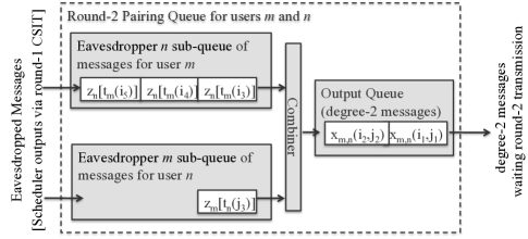
Figure 1: Sub-message pairing into degree-2 messages for user pair $(m,n)$.

To illustrate the difference between the two schemes consider first the problem of scheduling round-2 transmissions for a 2-round $K$-user MU-MIMO packet-centric scheme. This scheme relies on the use of a set of $(m,n)$ user-terminal pairing queues of the form shown in Fig 1, which generate degree-2 messages for round-2 transmissions. The main principles behind packet-centric eavesdropper-based scheduling can be summarized as follows:

1. Each round-1 slot involves transmitting a $K$ dimensional message intended for one of the $L$ users.

2. For each round-1 transmission intended for a given user, say user $m$, the base-station chooses $K-1$ out of the $L-1$ eavesdroppers for round-2 transmissions (based on round-1 eavesdropper CSIT).

3. For each such eavesdropper, e.g. eavesdropper $n$, the base-station places the eavesdropped observation of user $n$ in the corresponding $(m,n)$ queue, in the queue input associated with eavesdropper $n$.

4. Degree-2 messages for the user pair $(m,n)$ are formed by combining sub-messages from the queues of eavesdroppers $n$ and $m$ within the $(m,n)$ queue. These messages then simply wait for (round-2) transmission.

It is interesting to contrast eavesdropper scheduling with MAT-sessions scheduling in the case $K=2$. In this case, and given CSIT (from all users) from the round-1 transmission of message $i$ for user $m$, the eavesdropper scheduler in step 2) above selects one eavesdropper out of all the users via

$$\tilde{n}^{*}(m,i)={{\rm arg}\max}_{{\tiny n:1\leq n\leq L,\ n\neq}}\bar{R}_{m,i}(n)$$ (64)

where $\bar{R}_{m,i}(n)$ is a heuristic objective function obtained by replacing $\|{\bf h}^{\sf H}_{m}[t_{n}(j)]\|$ with $\|{\bf h}^{\sf H}_{n}[t_{m}(i)]\|$ in (60):

$$\bar{R}_{m,i}(n)=\log({\hbox{det}}[I+\mathbf{\tilde{H}}_{m,n}\mathbf{\tilde{H}}^{\sf H}_{m,n}P/2])$$

with $$~{}~{}~{}~{}\mathbf{\tilde{H}}_{m,n} \!\!\!\!=\!\!\!\! \left[\begin{array}[]{c}\mathbf{h}_{m}[t_{m}(i)]\\ \frac{1}{\sqrt{1+\|{\bf h}^{\sf H}_{n}[t_{m}(i)]\|^{2}}}\mathbf{h}_{n}[t_{m}(i)]\end{array}\right]$$ (67)

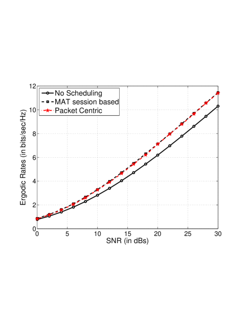
Figure 2: MAT-session based vs. packet-centric scheduling: the 2 user case.

Fig. 2 shows a performance comparison between the heuristic packet centric scheduler (64) and the MAT-based one (57), assuming $L=20$. As the figure illustrates, both schedulers yield nearly identical performance. Heuristic approximations of the form (64) can be readily used for implementing packet centric schedulers with $K$-user schemes. where $K>2$.

TABLE I: Sample 3-user 2-round MAT-Session Scheduling between packets 6, 13, and 27 of users 1, 2, and 3, respectively

Messages for:	${\bf x}_{1}(6)$	${\bf x}_{2}(13)$	${\bf x}_{3}(27)$
Round 1	${\bf x}_{1}(6)$	${\bf x}_{2}(13)$	${\bf x}_{3}(27)$
Round 2	​ ​${\bf x}_{1,2}(6,13)$​ ​${\bf x}_{1,3}(6,27)$​ ​	​ ​${\bf x}_{1,2}(6,13)$​ ​${\bf x}_{2,3}(13,27)$​ ​	​ ​${\bf x}_{1,3}(6,27)$​ ​${\bf x}_{2,3}(13,27)$​ ​

TABLE II: Sample 3-user 2-round Packet-Centric Scheduling for packets 6, 13, and 27 of users 1, 2, and 3, respectively

Messages for:	${\bf x}_{1}(6)$	${\bf x}_{2}(13)$	${\bf x}_{3}(27)$
Round 1	${\bf x}_{1}(6)$	${\bf x}_{2}(13)$	${\bf x}_{3}(27)$
Round 2	​ ​${\bf x}_{1,2}(6,13)$​ ​${\bf x}_{1,3}(6,27)$​ ​	​ ​${\bf x}_{1,2}(6,13)$​ ​${\bf x}_{2,4}(13,9)$​ ​	​ ​${\bf x}_{1,3}(6,27)$​ ​${\bf x}_{3,5}(27,4)$​ ​

Note that the DoFs of 2-round $K$-user packet-centric sessions are the same as the DoFs of the associated 2-round $K$-user MAT session. However, there is significantly more flexibility in scheduling eavesdroppers. Tables II and II provide examples of scheduling in a 2-round 3-user MAT session and of scheduling in a 2-round 3-user packet-centric approach. Both involve packet 6 of user 1, packet 13 of user 2, and packet 27 of user 3. The $i$-th column in each table shows all the transmitted messages associated with the packet of user $i$. As Table II shows, all transmissions in the MAT-session based scheme are determined by the scheduled MAT session involving the three user-packets. In contrast and as Table II shows, in the packet-centric scheme, the packets of user 2 (and 3) are no longer restricted to be included in transmissions involving packets of user 1 and 3 (1 and 2). Rather, the eavesdroppers in each case are chosen independently, and it is up to the pairing queue to group them into degree-two messages.

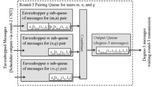
Figure 3: Sub-message combining into degree-3 messages for users $(m,n,q)$.

The preceding two-round schemes can readily extended to develop $R$-round $K$-user packet-centric schemes. As an example, consider the 3-round 3-user scheme. In this case, round-2 scheduling uses pairing queues of the form of Fig. 1 and works as already described. Round-3 scheduling amounts to scheduling eavesdroppers for degree-2 messages, i.e., messages simultaneously useful to 2 users. Given eavesdropper CSIT from round-2 transmissions intended for a particular pair of users $(m,n)$, an eavesdropper is selected, e.g. user $q$, out of all $L-2$ eavesdroppers. This eavesdropper’s message enters a round-3 pairing queue where it is used to create degree-3 messages for transmission. In particular, it is an input to the user $q$ eavesdropper queue of the $(m,n,q)$ message queue, shown in Fig. 3. As shown in the figure, degree-3 messages (messages simultaneously useful to a triplet of users $(m,n,q)$) are constructed by combining three eavesdropped observations of degree-two messages, one for each user eavesdropping on a message intended for the pair of remaining users.

V Simulation Results

In this section we provide a brief performance evaluation of the MU-MIMO schemes based on outdated CSI. We first provide a comparison between the MAT scheme and a conventional MU-MIMO scheme employing LZFB in the context of training and feedback over time-varying channels. We assume a block fading channel model that evolves according to a Gauss Markov process. The effect of the delay between the time $t_{pl}$ of downlink pilots (slots in which CSIT is estimated) and the time $t_{pl}+t_{\delta}$ of MU-MIMO transmission is captured by the magnitude of the expected correlation between channels from such a pair of time slots. This coefficient is defined by

$$\rho(t_{\delta})=\left|\mbox{\bb E}_{t}\left[{\bf h}_{k}^{{\sf H}}[t]{\bf h}_{k}[t+t_{\delta}]\right]\right|/\,\mbox{\bb E}_{t}\left[\|{\bf h}_{k}[t]\|^{2}\right]$$

A value $\rho=1$ means that the channels are perfectly correlated (co-linear), which happens if the CSI acquisition and data transmission occur in the same coherence block, whereas $\rho<1$ indicates that the channels changed between slots.

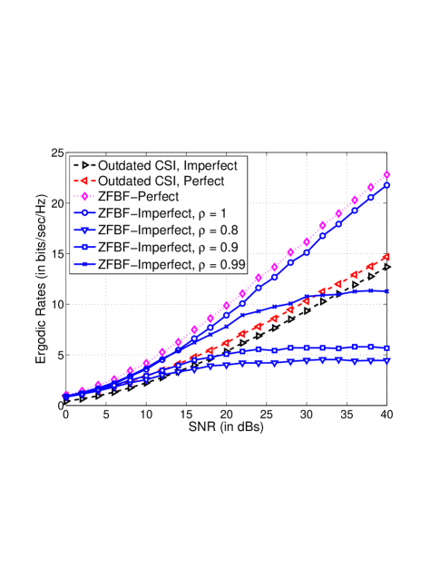
Figure 4: Comparison between MAT and conventional LZFB for a system with 2 antennas at the BS serving two single-antenna users.

Fig. 4 shows a comparison between the conventional LZFB and the MAT scheme for the case of $M=K=2$ in the presence of training, and assuming $\beta_{1}=\beta_{f}=2$ and $P=P_{1}$. When $\rho=1$ LZFB achieves 2 DoFs, as expected [7]. There is a constant rate gap between the perfect CSI case and the case of imperfect CSI based on training, as justified in [7]. In contrast for all cases with $\rho<1$, even with a very high correlation of $\rho=0.99$, the achievable rates eventually saturate as SNR increases [7]. Furthermore, decreasing $\rho$ below $0.99$ results in significantly lower saturation rates.

This rate saturation is not seen with the MAT schemes, which achieve DoF=$\frac{4}{3}$ independent of $\rho$. Using downlink training and CSI feedback degrades the achievable rate, however it does so by a constant gap regardless of the value $\rho$ and similar to what was observed in [7] for LZFB when $\rho=1$.

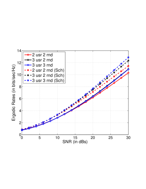
Figure 5: Performance of packet-centric scheduling in the case of two-user and three-user packet-centric MU-MIMO schemes based on outdated CSI.

Fig. 5 shows some of the benefits of packet-centric scheduling as a function of the number of users served by the MU-MIMO scheme and the number of rounds used for transmission. In particular, the figure shows a performance comparison of the “packet-centric” based scheduler for $K=3$ users with two and three rounds of transmission, as well as the scheduler’s performance for the $K=2$ user case. Also shown in the figure is the performance of the associated MAT-session based schemes without scheduling. As the figure suggests, the packet centric scheduler achieves the DoFs promised by the associated MAT scheme. In addition, packet-centric scheduling offers more flexibility when scheduling users, enabling performance benefits to be realized with a 3-round 3-user scheme at lower SNRs.

VI Conclusion

In this paper we considered training and scheduling aspects of multi-round MU-MIMO schemes that rely on the use of outdated channel state information (CSI) [8]. Such schemes are of practical interest as they enable one to rethink many operational aspects of deploying MU-MIMO in dynamic channel conditions, conditions which can inherently limit conventional MU-MIMO approaches. As shown in the paper, under proper training, the degrees of freedom promised by these schemes can be realized even with fully outdated CSI. We also proposed a novel scheduling algorithm that improves the performance of the original MAT scheme [8]. It is based on a variant multi-user MIMO scheme which maintains the MAT scheme DoFs but provides more scheduling flexibility. As our results suggest, an appropriately designed MU-MIMO scheme based on multi-round transmissions and outdated CSI can be a promising technology for certain practical applications.

References

- [1] G. Caire and S. Shamai, “On the achievable throughput of a multiantenna Gaussian broadcast channel,” IEEE Trans. on Info. Th., vol. 49, no. 7, pp. 1691–1706, 2003.
- [2] P. Viswanath and D. Tse, “Sum capacity of the vector Gaussian broadcast channel and uplink-downlink duality,” IEEE Trans. on Info. Th., vol. 49, no. 8, pp. 1912–1921, 2003.
- [3] S. Vishwanath, N. Jindal, and A. Goldsmith, “Duality, achievable rates, and sum-rate capacity of Gaussian MIMO broadcast channels,” IEEE Trans. on Info. Th., vol. 49, no. 10, pp. 2658–2668, 2003.
- [4] W. Yu and J. Cioffi, “Sum capacity of Gaussian vector broadcast channels,” IEEE Trans. on Info. Th., vol. 50, no. 9, pp. 1875–1892, 2004.
- [5] H. Weingarten, Y. Steinberg, and S. Shamai, “The capacity region of the Gaussian multiple-input multiple-output broadcast channel,” IEEE Trans. on Info. Th., vol. 52, no. 9, pp. 3936–3964, 2006.
- [6] T. Yoo and A. Goldsmith, “On the optimality of multiantenna broadcast scheduling using zero-forcing beamforming,” IEEE J. Select. Areas Commun., vol. 24, no. 3, pp. 528–541, March 2006.
- [7] G. Caire, N. Jindal, M. Kobayashi, and N. Ravindran, “Multiuser MIMO achievable rates with downlink training and channel state feedback,” IEEE Trans. on Info. Th., vol. 56, no. 6, pp. 2845–2866, June 2010.
- [8] M. Maddah-Ali and D. Tse, “Completely stale transmitter channel state information is still very useful,” in Proc. 48th Allerton Conf. Commun., Control and Computing, Monticello, IL, Oct. 2010, pp. 1188–1195.
- [9] H. Shirani-Mehr, G. Caire, and M. J. Neely, “MIMO downlink scheduling with non-perfect channel state knowledge,” IEEE Trans. on Commun., vol. 58, no. 7, pp. 2055–2066, July 2010.