Confinement of semiflexible polymers

Abstract

A variational framework is developed to examine the equilibrium states of a semiflexible polymer that is constrained to lie on a fixed surface. As an application the confinement of a closed polymer loop of fixed length $2\pi R$ within a spherical cavity of smaller radius, $R_{0}$, is considered. It is shown that an infinite number of distinct periodic completely attached equilibrium states exist, labeled by two integers: $n=2,3,4,\dots$ and $p=1,2,3,\cdots$, the number of periods of the polar and azimuthal angles respectively. Small loops oscillate about a geodesic circle: $n=2$, $p=1$ is the stable ground state; states with higher $n$ exhibit instabilities. If $R\geq 2R_{0}$ new states appear as oscillations about a doubly covered geodesic circle; the state $n=3,p=2$ replaces the two-fold as the ground state in a finite band of values of $R$. With increasing $R$, loop states make a transition from oscillatory and orbital behavior on crossing the poles, returning to oscillation upon collapse to a multiple cover of a geodesic circle (signaled, respectively, by an increase in $p$ and an increase in $n$). The force transmitted to the surface does not increase monotonically with loop size, but does asymptotically. It behaves discontinuously where $n$ changes. The contribution to energy from geodesic curvature is bounded. In large loops, the energy becomes dominated by a state independent contribution proportional to the loop size; the energy gap between the ground state and excited states disappears.

Instituto de Ciencias Nucleares, Universidad Nacional Autónoma de México
Apdo. Postal 70-543, 04510 México, DF, MEXICO

1 Introduction

Understanding how surfaces may constrain the configuration of biopolymers on mesoscopic scales is important in a number of processes in cell biology. It is particularly relevant in the packing of DNA within viral envelopes [1, 2]. Modeling all of the relevant interactions is complicated: one needs to accommodate the competition between polymer elasticity and entropy; in the case of DNA, electric fields will be important. A nice short review in this context is provided in [3]. Recently, simulations treating various features of the confinement process have been performed [4, 5]; the former focuses on entropy, the latter on the dramatic effects of friction and the finite transverse dimensions of the confined object.

In this paper, we address an aspect of the problem of a fundamental nature that does not appear to have been addressed previously in any detail: how does one characterize the equilibrium states of the three-dimensional elastic energy of a polymer confined within a fixed surface? While this description of confinement leaves out a lot of the physics that is relevant in biological systems, it presents a well-defined problem exhibiting a striking level of complexity that is worth studying in its own right.

The semi-flexible polymer will be modeled as a curve in three-dimensional space parameterized by arc-length $s$. The bending energy associated with a given conformation is quadratic in the Frenet-Serret curvature along the curve, $\kappa(s)$,

$$H=\frac{1}{2}\int ds\,\kappa(s)^{2}\,.$$ (1)

Curves of fixed length minimizing the unconstrained energy (1) were first studied in depth by Euler. A historical review is provided in Ref. [6]; a more contemporary approach to the problem is presented in [7, 8] and reviewed in Ref. [9]. An alternative framework, which lends itself to adaptation to the confinement problem, was developed in Ref. [10].

In the absence of constraints on a closed loop, there is not a lot to say: the only stable equilibrium is a circle. Confinement within a surface, however, will generally oblige the loop to adopt a non-circular shape, increasing its elastic energy. The contact with the surface itself may be complete or it may be partial; and contrary to one’s initial guess, the bound state will not generally follow a surface geodesic; nor need it be unique.

The wrapping of a semi-flexible polymer around a cylinder, a closely related problem relevant in the the winding of DNA around histone octamers, was first examined some time ago by Nickerson and Manning [11, 12]. Their strategy was to look at the independent degrees of freedom of the surface-bound polymer. While focusing directly on these degrees of freedom makes sense, it does not exploit the symmetries of the problem. For, even though the constraint breaks the Euclidean invariance of the three-dimensional bending energy, how this occurs is not arbitrary. A variational framework is developed here that involves the unconstrained degrees of freedom, imposing the constraint using a local Lagrange multiplier. This multiplier will quantify the loss of Euclidean invariance in the constrained system. Its value at any point along the loop will be identified as the local normal force that is being transmitted to the surface.

The well-known integrability of the Euler-Lagrange equations for the unconstrained curve is a consequence of the Euclidean invariance of its energy. The constrained counterpart generally will not be integrable. In various interesting cases, however, the confining geometry will respect some subgroup of the Euclidean group. In particular, the conservation of torque associated with the residual rotational invariance of a sphere permits the Euler-Lagrange equation to be cast as a quadrature in the geodesic curvature which can be integrated directly. It also provides a direct recipe for the reconstruction of the loop from its curvature data adapted to the conserved torque vector as an axis of symmetry.

In particular, we apply this framework to examine the confinement of a closed polymer loop of fixed length $2\pi R$ within a sphere of radius $R_{0}\leq R$.

In contrast to an open polymer which will wind around a geodesic circle on the sphere when its length exceeds $\pi R_{0}$, the closure of the loop is incompatible with a geodesic unless $R$ is tuned to be commensurate with an integer multiple of $R_{0}$. We show that there exists an infinite number of distinct completely attached states, labeled by a pair of integers, $n$ and $p$: $n=2,3,4\dots$, $p=1,2,3,\dots$, the number of periods of the polar angle and azimuthal angles in one circuit of the loop respectively. $n$ characterizes the dihedral symmetry with respect to the axis of symmetry; $p$ characterizes the number of revolutions about this axis. Small loops oscillate symmetrically about a geodesic circle with $p=1$ and an $n$-fold symmetry, $n=2,3,\dots$. The two-fold is the stable ground state. For any finite values of $R$, the higher $n$-folds are unstable with respect to decay toward the two-fold. States with $n=2$ are illustrated in Figs. 1(a) - 1(c) for various normalized values of $R$.

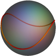
(a) $R=1.1$

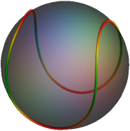
(b) $R=1.5$

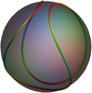
(c) $R=2$

(d) $R=2.127$

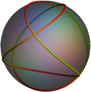
(e) $R=2.5$

(f) $R=2.99$

Figure 1: (Color online) State with two-fold symmetry for values of $R$ in the interval $[1,3]$ within a unit sphere: (a) and (b) display increasingly large oscillations about the equator; (c) oscillations develop overhangs; (d) first self-contacts made at the two poles; (e) self-intersecting triple orbit of sphere; (f) orbit collapses to triple cover of the equator. The normalized local confining force $\lambda$ is color coded in these figures.

Beyond some critical size, the loop will exhibit self-intersections on the sphere. When $n=2$ this will occur when $R=2.127R_{0}$ where the loop crosses the poles as illustrated in Fig. 1(d). We suppose that self-intersections are consistent with the physics and do not cost energy.

As $R$ is increased to $R=3R_{0}$, the loop will collapse onto a geodesic circle which it will cover three times, (see Figs. 1(e) and 1(f). The discontinuity in the number of revolutions occurs at an intermediate value of $R$ where the loop crosses the poles. This is accompanied by a transition from oscillatory to orbital behavior. As $R$ is increased above $3R_{0}$, the dihedral symmetry of the lowest energy state descending from the $n=2$ ground state will jump to $n=4$ with the reestablishment of oscillatory behavior.

The bending energy of this state as well as the total force that gets transmitted to the surface will be determined as a function of $R$. The three- dimensional bending energy decomposes on the surface into a sum of two terms: one is associated with the geodesic curvature, intrinsic to the sphere; the other is associated with the normal curvature inherited from the surface, constant on a sphere. The latter energy thus counts the number of times the loop is wound within the sphere and it is proportional to $R$. The geodesic energy periodically falls to zero whenever $R=pR_{0}$ and the loop is geodesic. Local maxima, associated with the incommensurability of the loop length with geodesic behavior, are displayed between these values; we show that their values decrease monotonically with loop size. For large values of $R$, the normal contribution is always dominant. It does not depend on the state in question. Thus, in this limit, the energy gap between the ground state and excited states disappears. The local force transmitted by the completely attached ground state loop is positive everywhere. Surprisingly, the total force does not grow monotonically with loop length except asymptotically, where it grows linearly with $R$ and coincides with the naive expression, energy divided by $R_{0}$. The change of symmetry as $R$ passes through odd integral multiples of $R_{0}$, manifests itself in a positive jump in the transmitted force analogous to a Euler instability associated with the buckling into oscillations.

When $R\geq 2R_{0}$, a new set of states appears as oscillations about a doubly covered geodesic circle, $p=2$ with an $n$-fold symmetry, $n=3,4,5,\dots$; among these new states, the lowest energy is displayed in the three-fold. Also, because the geodesic energy is small when the oscillations are small, these states will have lower energy than the two-fold ground state in a finite band of values of $R$ beginning at $2R_{0}$. There will be similar behavior in an infinite set of bands of values of $R$ where the descendant states become geodesic. One thus needs to reassess the stability of the two-fold ground state and its descendants. We provide a heuristic argument for stability by constructing a homotopy that interpolates between the states with $n=2$, $p=1$ and $n=3$, $p=2$. By examining the energy along this homotopy, we show that a steep energy barrier separates the two equilibrium states. The $n=2$, $p=1$ state and its descendants thus appear to be stable classically. For any $R\geq 2R_{0}$, there are two stable states that alternate as the ground state as the length is increased.

The paper is organized as follows: In section 2, we describe the framework. In particular, the breaking of translational invariance will be quantified by the non-conservation of a vector along the loop. It will be shown that the Euler-Lagrange equation for the curve can be cast as the vanishing of a linear combination of the unconstrained Euler-Lagrange derivatives. The constraining force is identified as some other linear combination of these derivatives. In Sect. 3 the confinement of a closed loop by spheres will be considered. In Secs. 4 and 5 we analyze loops in the harmonic and non-linear regimes respectively. The equilibrium states of the loop will be identified and the forces they transmit to the surface determined. An assessment of the stability of these states will be provided. We conclude with a discussion and a few suggestions for future work in Sec. 6. A number of useful definitions, identities and derivations are collected in a set of appendixes.

2 Curves constrained to surfaces

Consider a space curve $\Gamma:s\rightarrow\mathbf{Y}(s)$ parametrized by arclength constrained to lie on a surface $\Sigma$. This surface is described in parametric form by the mapping $\Sigma:(u^{1},u^{2})\rightarrow\mathbf{X}(u^{1},u^{2})$. The confined curve can then also be described as a surface curve $\Gamma_{\Sigma}:s\rightarrow(U^{1}(s),U^{2}(s))$. In order to enforce the condition that $\Gamma$ lie on $\Sigma$, one adds to the energy $H[\mathbf{Y}]$ given by Eq. (1) a term enforcing this constraint:

$$H_{c}[\mathbf{Y},U^{a}]=H[\mathbf{Y}]+\int\,ds\,\,\bm{\lambda}(s)\cdot\left[\mathbf{Y}(s)-\mathbf{X}(U^{a}(s))\right]\,,$$ (2)

where $\bm{\lambda}$ is a vector-valued Lagrange multiplier defined along the curve. This constraint will break the manifest translational invariance of the energy $H$.

The variation of $H_{c}$ with respect to the embedding functions $\mathbf{Y}$ can be cast in the form

$$\delta_{\bf Y}H_{c}=\int ds\left(\mathbf{F}^{\prime}+{\bm{\lambda}}\right)\cdot\delta\mathbf{Y}\,,$$ (3)

where prime represents derivation with respect to arclength and the tension in the loop ${\bf F}$ is given by

$$\mathbf{F}=\left(\frac{1}{2}\kappa^{2}-c\right)\mathbf{T}+\kappa^{\prime}\mathbf{N}+\kappa\tau\mathbf{B}\,.$$ (4)

Here $\{{\bf T},{\bf N},{\bf B}\}$ is the standard Frenet-Serret frame carried by the curve and $\tau$ is its torsion. The constant $c$ is associated with the constraint of fixed length. A derivation of Eq. (4) is provided in Appendix A.

In equilibrium, one finds that $\mathbf{F}^{\prime}=-\bm{\lambda}$. Thus, in the presence of the constraint, the tension in the loop is not conserved; the multiplier is identified as the external force associated with the constraint [18].

The corresponding variation of $H_{c}$ with respect to $U^{a}(s)$ is given by

$$\delta_{U}H_{c}=-\int ds\,\bm{\lambda}\cdot\mathbf{e}_{a}\,\delta U^{a}\,,$$ (5)

where ${\bf e}_{a}$, $a=1,2$ are the two tangent vectors to the surface adapted to the parametrization by $u^{a}$. In equilibrium, $\bm{\lambda}\cdot{\bf e}_{a}=0$ ; in equilibrium, the force on the curve associated with the constraint always acts orthogonally to the surface. Let us write $\bm{\lambda}=\lambda\,\mathbf{n}$, where $\mathbf{n}$ is the unit vector normal to $\Sigma$. The combined result is that

$$\mathbf{F}^{\prime}=-\lambda\mathbf{n}\,.$$ (6)

An integrability condition for closed curves follows from Eq. (6):

$$\oint ds\,\lambda\,{\bf n}=0\,.$$ (7)

This identity holds whether or not contact is complete.

Using Eq. (4) along with the Frenet-Serret equations, a straightforward calculation decomposes ${\bf F}^{\prime}$ along the normals

$${\bf F}^{\prime}=\varepsilon_{\bf N}\mathbf{N}+\varepsilon_{\bf B}\mathbf{B}\,,$$ (8)

where the Euler-Lagrange derivatives of the bending energy $\varepsilon_{\bf N}$ and $\varepsilon_{\bf B}$ are given by

$$\varepsilon_{\mathbf{N}} = \kappa^{{}^{\prime\prime}}+\kappa\,\left(\frac{\kappa^{2}}{2}-\tau^{2}-c\right)\,,$$ (9a)

$$\varepsilon_{\mathbf{B}} = \frac{2}{\kappa}\,\left(\kappa^{2}\tau\right)^{\prime}\,.$$ (9b)

The tangential Euler-Lagrange derivative $\varepsilon_{\bf T}=\mathbf{F}^{\prime}\cdot\mathbf{T}$ vanishes identically, a consequence of the fact that the only relevant degrees of freedom are geometrical, whether the curve is constrained or not.

The surface-bound curve also carries a Darboux frame, $\{{\bf T},{\bf n},{\bf l}={\bf T}\times{\bf n}\}$. Relevant properties of this frame are summarized in Appendix B. The Frenet normals are related to their Darboux counterparts by a rotation about the tangent vector:

$${\bf N}=\cos\omega\,{\bf n}+\sin\omega\,{\bf l}\,;\quad{\bf B}=-\sin\omega\,{\bf n}+\cos\omega\,{\bf l}\,.$$ (10)

The relationship ${\bf T}^{\prime}=\kappa{\bf N}$ permits one to express the angle of rotation in terms of a curvature ratio: $\sin\omega=\kappa_{g}/\kappa$ or $\cos\omega=\kappa_{n}/\kappa$, where $\kappa_{g}$ and $\kappa_{n}$ are, respectively, the geodesic and normal curvatures along $\Gamma_{\Sigma}$,

$$\kappa_{g}={\bf T}^{\prime}\cdot{\bf l}\,,\quad\kappa_{n}={\bf T}^{\prime}\cdot{\bf n}\,.$$ (11)

Using these expressions it is possible to decompose ${\bf F}^{\prime}$ given by Eq. (8) in a form adapted to the surface,

$${\bf F}^{\prime}=\left(\cos\omega\,\varepsilon_{\bf N}-\sin\omega\,\varepsilon_{\bf B}\right)\mathbf{n}+\left(\sin\omega\,\varepsilon_{\bf N}+\cos\omega\,\varepsilon_{\bf B}\right)\mathbf{l}\,.$$ (12)

The projection of Eq. (6) onto $\mathbf{l}$ provides the Euler-Lagrange equation in the remarkably simple form,

$$\varepsilon_{\mathbf{l}}=\sin\omega\,\varepsilon_{\mathbf{N}}+\cos\omega\varepsilon_{\mathbf{B}}=0\,.$$ (13)

The multiplier $\lambda$ does not appear. The corresponding projection onto ${\bf n}$ determines $\lambda$,

$$\lambda=-\cos\omega\,\varepsilon_{\mathbf{N}}+\sin\omega\,\varepsilon_{\mathbf{B}}\,.$$ (14)

In this approach, one sees explicitly how both the Euler-Lagrange equation (13) and the confining force (14) are constructed out of the two unconstrained Euler-Lagrange derivatives. The normal force is completely determined when the local geometry is known.

The Euler-Lagrange equations for an unconstrained elastic curve, given by $\varepsilon_{\bf N}=0$ and $\varepsilon_{\bf B}=0$, are replaced by the single equation, $\varepsilon_{\bf l}=0$. The apparent discrepancy in the number of equations reflects the fact that a space curve possesses two independent modes of deformation whereas a surface curve has only one. In general, the integrability of the former pair of equations is surrendered when the constraint is present.

2.1 Euler-Lagrange equation in terms of surface curvatures

Using the identities (B.3) and (B.4) the Euler-Lagrange equation (13) can be expressed completely in terms of surface curvatures,

$$\varepsilon_{\mathbf{l}}=\kappa_{g}^{\prime\prime}+\kappa_{g}\left(\frac{\kappa_{g}^{2}+\kappa_{n}^{2}}{2}-\tau_{g}^{2}-c\right)-\frac{\left(\kappa^{2}_{n}\tau_{g}\right)^{\prime}}{\kappa_{n}}=0\,.$$ (15)

This agrees with the equation derived in Ref. [12] using a very different approach. Note that it involves the curvatures as well as the geodesic torsion and, in general, the curve will not follow a geodesic with $\kappa_{g}=0$. For a geodesic to minimize bending energy, one requires one of the following to occur: $\kappa_{n}^{2}\tau_{g}$ is constant; the curve coincides with an asymptotic line with $\kappa_{n}=0$ or a principal curve with $\tau_{g}=0$. Such conditions typically do not occur unless they do so trivially.

The magnitude of the force $\lambda$ transmitted to the surface, given by Eq. (14), assumes the form

$$-\lambda=\kappa_{n}^{\prime\prime}+\kappa_{n}\left(\frac{\kappa_{g}^{2}+\kappa_{n}^{2}}{2}-\tau_{g}^{2}-c\right)+\frac{\left(\kappa_{g}^{2}\tau_{g}\right)^{\prime}}{\kappa_{g}}\,.$$ (16)

Its magnitude will vary along the contact region, even for confinement by a sphere. This expression is missing in the framework presented in [12]. A curious consequence of the symmetric decomposition of the Frenet-Serret curvature in terms of the geodesic and the normal curvatures is the fact that $\lambda$ turns out to be identical to the Euler-Lagrange derivative $\varepsilon_{\mathbf{l}}$ given by (15) under the interchange of $\kappa_{g}$ with $\kappa_{n}$ and a change of sign of the last term.

2.2 Confinement and the loss of rotational invariance

In general, under confinement, one surrenders not only translational invariance but also rotational invariance. The torque about the origin per unit length of the curve, ${\bf M}$, is given by

$${\bf M}=\ {\bf Y}\times{\bf F}+{\bf S}\,,$$ (17)

where ${\bf S}=-\kappa{\bf B}=\kappa_{g}\,{\bf n}-\kappa_{n}\,{\bf l}$ . The first term on the right in Eq. (17) is the torque due to the force ${\bf F}$; the second term is the bending moment originating in second derivatives in the bending energy. For a free curve, ${\bf M}^{\prime}=0$, which can be cast in the manifestly translationally invariant form $\mathbf{S}^{\prime}+\mathbf{T}\times\mathbf{F}=0$ [18]. In general, ${\bf M}$ is not conserved. One has instead

$$\mathbf{M}^{\prime}=\varepsilon_{\mathbf{l}}\left(\mathbf{Y}\times\mathbf{l}\right)-\lambda\left(\mathbf{Y}\times\mathbf{n}\right)\,.$$ (18)

Thus, in a confined equilibrium with $\varepsilon_{\mathbf{l}}=0$, ${\bf M}$ will not generally be conserved. The source is given by the moment of the force associated with the constraint.

If the confining geometry is a sphere centered on the origin, so that $\mathbf{Y}$ is directed along the normal vector, ${\bf M}$ will be conserved. If it is symmetric about some axis (say the $z$ axis), then the conserved quantity is the corresponding projection of ${\bf M}$, that is, $M_{3}={\bf M}\cdot\hat{\bf z}$.

3 Spherical confinement

Consider a closed curve of length $S=2\pi R$, confined within a sphere of radius $R_{0}$. We normalize lengths in terms of $R_{0}$. On a sphere, the extrinsic curvature tensor is proportional to the metric $K_{ab}=g_{ab}$, so that the normal curvature is constant, $\kappa_{n}=-1$, and the geodesic torsion vanishes, $\tau_{g}=0$. Using Eq. (A.6), the vector $\mathbf{F}$ given by Eq. 4, then reduces to

$$\mathbf{F}=\left(\frac{\kappa_{g}^{2}}{2}+\sigma\right)\mathbf{T}+\kappa_{g}^{\prime}\mathbf{l}\,\qquad\text{where}\qquad\sigma=\frac{1}{2}-c\,.$$ (19)

${\bf F}$ is everywhere tangent to the surface. It is also completely determined by the intrinsic geometry. However, it is not conserved.

The torque vector defined by Eq. (17) is given by

$$\mathbf{M}=\kappa_{g}^{\prime}\mathbf{T}-\left(\frac{\kappa_{g}^{2}}{2}+\sigma-1\right)\mathbf{l}+\kappa_{g}\mathbf{n}\,.$$ (20)

The rotational invariance of bending energy confined to a sphere implies that ${\bf M}$ is a constant vector. In particular, its length is a constant. This provides a quadrature for the geodesic curvature ($M^{2}={\bf M}\cdot{\bf M}$):

$$M^{2}=(\kappa_{g}^{\prime})^{2}+\left(\frac{\kappa_{g}^{2}}{2}+\sigma-1\right)^{2}+\kappa_{g}^{2}\,.$$ (21)

It is simple to check that the condition $(M^{2})^{\prime}=0$ in Eq. (21) reproduces the Euler-Lagrange Eq. (15) on a sphere:

$$\varepsilon_{{\bf l}}=\kappa_{g}^{\prime\prime}+\kappa_{g}\left(\frac{\kappa^{2}_{g}}{2}+\sigma\right)=0\,.$$ (22)

This equation is also identical to the one describing an elastic loop on a sphere with an energy density, $\kappa_{g}^{2}/2$. The minimization of the constrained three-dimensional bending energy coincides in this case with that of two-dimensional spherical bending energy. This is a consequence of the decomposition of the Frenet-Serret curvature into normal and geodesic parts, $\kappa^{2}=\kappa_{g}^{2}+\kappa^{2}_{n}$ as well as the fact that $\kappa_{n}$ is a constant. Spheres are special in this respect.

Various mathematical properties of elastic curves on spheres were described by Langer and Singer in the 1980s [7]; see also [19] for a numerical treatment of the problem. Recently they have been reexamined in some detail in [20]. The connection to the description of conical defects in unstretchable flat sheets was developed in [21] and [22]. While the mathematical literature provides a useful point of departure, the absence of any reference either to energy or to the transmitted forces limits its usefulness.

Note that in a geodesic, $\kappa_{g}=0$ everywhere. Equation (21) then implies that $M^{2}=(\sigma-1)^{2}$. Unless $R$ is an integer, however, geodesics will be inconsistent with the boundary conditions associated with closure. If $\kappa_{g}=0$ is accessible anywhere along the loop, there will be a non-trivial bound on $M$ from below:

$$(\sigma-1)^{2}\leq M^{2}\,.$$ (23)

In equilibrium, all confined loops will satisfy this bound.

It is also useful to cast Eq. (21) in the alternative form

$$(\kappa_{g}^{\prime})^{2}+V(\kappa_{g})=E^{2}\,,$$ (24)

where

$$V(\kappa_{g})=\left(\frac{\kappa_{g}^{2}}{2}+\sigma\right)^{2}\,,$$ (25)

and $E^{2}=M^{2}+2\sigma-1$ is manifestly positive.

If $\kappa_{g}$ is identified as the position of a particle and $s$ as time, then Eq. (24) described the motion of a particle of mass $m=2$ and total “energy” $E^{2}$ in the symmetric quartic potential $V(\kappa_{g})$. If $\sigma\geq 0$, $V$ possesses a single minimum at $\kappa_{g}=0$; if $\sigma<0$ it possesses two symmetric wells centered at $\kappa_{g}=\pm\sqrt{-2\sigma}$, separated by a local maximum at $\kappa_{g}=0$.

While the particle analogy is useful, it does have its limitations. $E^{2}$ also is not the energy of the loop and the potential depends on the constant of integration $\sigma$ which we are not free to tune but, like the ‘energy’, is itself determined by the boundary conditions.

The qualitative behavior of the loop will depend on the turning points of the potential, and thus on the relative values of $\sigma^{2}$ and $E^{2}$:

(1) $E^{2}>\sigma^{2}$ (equivalently Eq. (23) is satisfied). In this parameter regime, there are only two turning points. One has

$$E^{2}-V(\kappa_{g})=\frac{1}{4}\left(\kappa^{2}_{g}+K^{2}\right)\left(k_{1}^{2}-\kappa^{2}_{g}\right)\,,$$ (26)

where $K^{2}=2(E+\sigma)\geq 0$ and $k_{1}^{2}=2(E-\sigma)\geq 0$. Thus $\kappa_{g}^{\prime}=0$ when $\kappa_{g}=\pm k_{1}$. The geodesic curvature thus ranges in the symmetric interval $[-k_{1},k_{1}]$. This will be independent of the sign of $\sigma$. The loop will oscillate symmetrically about the equator where $\kappa_{g}=0$ (see Eq. (29)) so that $\oint ds\kappa_{g}=0$.

(2) $E^{2}<\sigma^{2}$. This regime is inaccessible physically if the loop is closed.

The reconstruction of the loop from its curvature data involves examining the conserved torque vector ${\bf M}$. Without loss of generality, it is always possible to allign $\mathbf{M}$ along the $\hat{\mathbf{z}}$ axis, $\mathbf{M}=M\hat{\mathbf{z}}$ (we follow Ref. [22]). The normal vector $\mathbf{n}$ is parametrized in terms of spherical polar coordinates $\vartheta$ and $\varphi$,

$$\mathbf{n}(s)=\left(\sin\vartheta(s)\cos\varphi(s),\sin\vartheta(s)\sin\varphi(s),\cos\vartheta(s)\right)\,.$$ (28)

The projection of $\mathbf{M}$, given by Eq. (20), onto ${\bf n}$ determines the polar angle in terms of $\kappa_{g}$:

$$\mathbf{M}\cdot\mathbf{n}=M\cos\vartheta=\kappa_{g}\,;$$ (29)

its projection onto $\mathbf{l}$ determines the azimuthal angle $\varphi$

$$\mathbf{M}\cdot\mathbf{l}=-M\sin^{2}\vartheta\varphi^{\prime}=-\left(\frac{\kappa^{2}_{g}}{2}+\sigma-1\right)\,.$$ (30)

Thus the projections of $\mathbf{M}$ onto the Darboux frame determine the embedding functions of the curve on the sphere in terms of $\kappa_{g}$ and the two constants, $\sigma$ and $M$.

$\varphi$ will not generally increase monotonically along the loop. It will exhibit overhangs with $\varphi^{\prime}=0$, if $\sigma\leq 1$. Combining Eqs. (29) and (30) gives

$$\varphi^{\prime}=\frac{M}{2}\,\left(\frac{M^{2}+2(\sigma-1)}{M^{2}-\kappa_{g}^{2}}-1\right)\,.$$ (31)

Note that Eq. (29) implies the bound on $\kappa_{g}$, $|\kappa_{g}|\leq M$, already implicit in the quadrature, Eq. (21). As we will see, $M$ will always be bounded. Thus $\kappa_{g}$ and with it the geodesic energy will also be bounded. Equation (29) also implies that the extremal values of $\kappa_{g}$ occur where the polar angle is turning. The bound is saturated when the loop passes through the poles.

Using the identification, (29), it is possible to recast the quadrature in terms of $\theta$. One has

$$\theta^{\prime}{}^{2}+\frac{1}{M}\left(\frac{M^{2}+2(\sigma-1)}{\sin\theta}-M^{2}\sin\theta\right)^{2}=1\,.$$ (32)

In this form, it is clear that access to the poles is possible only when $M$ and $\sigma$ are tuned so that the coefficient of the divergent term in the potential appearing in Eq. (32) vanishes:

$$M^{2}+2(\sigma-1)=0\,.$$ (33)

This will require $\sigma<1$.

When Eq. (33) is satisfied, the evolution of $\varphi$ simplifies. Equation (31) assumes the form $\varphi^{\prime}=-M/2$ so that $\varphi$ increases linearly with arclength along the loop. In general, the dependence of $\varphi$ on $s$ is not monotonic, much less linear. This identity, in turn, implies the value $M=2/R$ (and as a consequence of Eq. (33), $\sigma=1-2/R^{2}$ at pole crossing.

Let us first suppose that the loop is sufficiently small so that neither self-contact nor self-intersections occur. The periodic motion in the potential $V(\kappa_{g})$ implies an $n$-fold dihedral symmetry: the loop closes upon completing $n$ periods of $\theta$ in one revolution of the polar axis so that $\theta(s+2\pi R/n)=\theta(s)$ and $\varphi(s+2\pi R/n)=\varphi(s)+2\pi/n$, where $n\geq 2$ is an integer. Closure provides a quantization of physical states.

In equilibrium, the number of circuits of the polar axis, $p$, will increase with loop length, so that the boundary condition on $\varphi$ is replaced with $\varphi(s+2\pi R/n)=\varphi(s)+2\pi p/n$. Using Eqs. (29) and (31), and the quadrature (24) it is possible to cast the boundary conditions in the form

$$\frac{2\pi R}{4n}=\int_{0}^{k_{1}}\frac{d\kappa_{g}}{\sqrt{E^{2}-V(\kappa_{g})}}\,,$$ (34)

and

$$\frac{2\pi p}{4n}=\frac{M}{2}\,\int_{0}^{k_{1}}\frac{d\kappa_{g}}{\sqrt{E^{2}-V(\kappa_{g})}}\,\frac{\kappa_{g}^{2}+2(\sigma-1)}{M^{2}-\kappa_{g}^{2}}\,,$$ (35)

where $k_{1}$ is the turning point of the potential, defined by Eq. (26). Equation (34) is independent of $p$, whereas Eq. (35) is independent of $R$. Together, they determine the two constants of integration $\sigma$ and $M$ in terms of the loop radius $R$ and the two integers $n$ and $p$.

4 Weak confinement by Spheres

While Eq. (21) can be integrated exactly in terms of elliptic functions [7, 9, 20]), a perturbative approach to the problem is instructive. Let us thus suppose that $\Delta R:=R-1\ll 1$. Such a loop is sufficiently small that neither self-contact nor self-intersections occur. We thus expand the function $\kappa_{g}$ as well as the constants $\sigma$ and $M$ in powers of $\epsilon=\sqrt{\Delta R}$, the small dimensionless parameter in the problem:

$$\kappa_{g}=\kappa_{1}+\kappa_{3}+\cdots\,;\quad M=M_{0}+M_{2}+\cdots\,;\quad\sigma=\sigma_{0}+\sigma_{2}+\cdots\,.$$ (36)

The equilibrium states are described by small oscillations about a geodesic circle on the sphere with $\kappa_{g}=0$. The harmonic approximation of the quadrature (21) about $\kappa_{g}=0$ reads

$$(\kappa_{1}^{\prime})^{2}+\sigma_{0}\kappa_{1}^{2}=M_{0}^{2}-(\sigma_{0}-1)^{2}+2M_{0}M_{2}-2\sigma_{0}\sigma_{2}\,.$$ (37)

At lowest order, the arclength coincides with the azimuthal angle, $\varphi$, and the geodesic curvature along a closed loop is given by

$$\kappa_{1}(s)\approx A_{1}\cos n\varphi\,,$$ (38)

where $n$ is an integer and $A_{1}$ is a constant. $\Delta R$ is determined by the amplitude $A_{1}$ and the $n$ (see Appendix C).

The quadrature implies that $\sigma_{0}=n^{2}$ and $M_{0}=n^{2}-1$. It also implies the constraint

$$\frac{2}{n^{2}}(n^{2}-1)(M_{2}-\sigma_{2})=A_{1}^{2}$$ (39)

on the difference of their second order corrections.

Equation (38) implements the boundary conditions at lowest order. To complete the specification of $\sigma_{2}$ and $M_{2}$ in terms of $\Delta R$, it is necessary to examine the boundary conditions (34) and (35) correct at next to leading order. One finds that, for $n\geq 2$, Eqs. (34) and (35) together imply

$$\Delta R=-\frac{1}{4n^{4}}(\sigma_{2}-M_{2})-\frac{1}{4n^{2}}(\sigma_{2}+M_{2})-\frac{1}{16n^{2}}A_{1}^{2}\,,$$ (40)

and

$$\Delta R=-\frac{1}{n^{2}-1}(\sigma_{2}-M_{2})-\frac{1}{4(n^{2}-1)}\frac{n^{2}+1}{n^{2}-1}\,A_{1}^{2}\,.$$ (41)

The details of the derivation are provided in Appendix C. Using Eq. (39) in (41) one reproduces the relationship Eq. (C.4) between $A_{1}$ and $\Delta R$, $A_{1}^{2}=4(n^{2}-1)\Delta R$. It then follows that, for $n\neq 1$,

$$\sigma_{2}=\frac{1}{2}(3-7n^{2})\Delta R\,,\quad M_{2}=\frac{3}{2}(1-n^{2})\Delta R\,.$$ (42)

4.1 Energy and transmitted force

The bending energy of the loop confined by the sphere decomposes into a sum of geodesic and normal parts, reflecting the decomposition of the Frenet curvature, $\kappa^{2}=\kappa_{g}^{2}+1$,

$$H=\frac{1}{2}\oint ds\left(\kappa^{2}_{g}+1\right):=H_{g}+H_{n}\,.$$ (43)

$H_{n}=\pi R$ is the energy associated with an elastic rod that been wound into a circular coil of radius $R_{0}=1$. It grows linearly with loop length $2\pi R$ and is state independent. For a weakly confined loop

$$H/H_{\sf loop}\approx 1+2n^{2}\Delta R\,,$$ (44)

where $H_{\sf loop}=\pi/R$ is the bending energy of a circular loop of radius $R$. The energy increases linearly with loop size. This will not be true in longer loops.

For a fixed value of $\Delta R$, the energy increases quadratically with $n$. The ground state, as one would have predicted, is the completely attached $n=2$ state. As we show, all states with $n\geq 3$ are unstable.

The force transmitted to the sphere at any point, given in Eq. (16), takes the particularly simple form

$$\lambda=\frac{1}{2}\,\kappa^{2}_{g}+\sigma\,.$$ (45)

It differs from the local energy density: compare Eqs. (43) and (45). Its spatial dependence is completely determined by the geodesic curvature. It is bounded from below by $\sigma$. This lends a direct physical interpretation of $\sigma$. For small $\Delta R$ and each $n\geq 2$, the force is given by

$$\lambda_{n}\approx n^{2}+\frac{\Delta R}{2}\left[3-7n^{2}+4\left(n^{2}-1\right)\cos^{2}\,n\varphi\right]\,;$$ (46)

while it oscillates along the loop, it remains positive everywhere. $\lambda_{n}$ does not vanish in the limit $\Delta R\to 0$. This is interpreted as an Euler instability. The buckling of the circular loop into an $n$-fold involves a critical compression in the loop provided by this normal force. Thereafter, $\lambda_{n}$ decreases linearly with $\Delta R$. This may appear counterintuitive. This behavior will be put in context when we examine loops outside of perturbation theory.

4.2 Stability

Here we examine the stability of the weakly confined $n$-folds that have been described. To do this we require the second variation of the energy with respect to small deformations of the loop. This is expressed in the form [23]

$$\delta^{2}H=\int d\varphi\,\Phi{\cal L}\Phi\,,$$ (47)

where $\Phi$ is the deformation along ${\bf l}$, and the self-adjoint operator ${\cal L}$ is given by

$${\cal L}=\frac{\partial^{4}}{\partial\varphi^{4}}+(n^{2}+1)\,\frac{\partial^{2}}{\partial\varphi^{2}}+n^{2}\,.$$ (48)

The fixed length constraint along the spherical surface implies a global constraint on the normal deformation,

$$\oint ds\kappa_{g}\Phi=0\,.$$ (49)

Periodicity implies that the modes of deformation are represented by a constant ($m=0$), $\sin m\varphi$ and $\cos m\varphi$, $m=1,2,3,\dots$. For fixed $n$, the eigenvalues of ${\cal L}$ are then labeled by the integer $m=0,1,2,\dots$, given by

$$C_{m}=(m^{2}-n^{2})(m^{2}-1)\,.$$ (50)

The constant mode with $m=0$ has positive $C_{0}=n^{2}$. All eigenvalues with $m\geq 1$ possess a two-fold degeneracy.

There are four zero modes satisfying ${\cal L}\Phi=0$; two occur at $m=1$ and two at $m=n$. The mode $\sin n\varphi\propto\kappa_{g}^{\prime}$ corresponds to rotation of the loop about the axis of symmetry. The two modes with $m=1$ correspond to rotations about an orthogonal axis. These three modes are the zero modes anticipated by the rotational invariance of the bending energy. The fourth zero mode $\cos n\varphi$ is inconsistent with the fixed length constraint (49) and, so, is unphysical. It is also the only mode of deformation inconsistent with this constraint in this regime.

The two-fold ground state with $n=2$ is stable. There are no modes of deformation with negative eigenvalue.

All excited confined states are unstable. There will be $2(n-2)$ unstable modes of deformation corresponding to $m=2,\dots,n-1$ lying between the zero modes at $m=1$ and $m=n$. All modes of deformations with $m>n$ contribute a positive energy. The first excited state with $n=3$ has two modes of decay, of equal energy, into the ground state. The dominant mode of instability in higher energy states is not directly towards the ground state involving a cascade of instabilities.

5 Strong spherical confinement

Let us now examine the shape adopted by a loop of finite $R$ confined by the sphere.

Equation (22) can be integrated in terms of elliptic functions to give $\kappa_{g}$ as a function of $s$ [7, 9, 20]

$$\kappa_{g}(s)=\kappa_{0}\,\text{cn}\,\left[qs,m\right]\,,\qquad\kappa_{0}=2\sqrt{m}q\,.$$ (51)

The function $\text{cn}[x,m]$ is the Jacobi elliptic cosine [24]. The angular wavenumber $q$ is given in terms of the constant $E$ defined below Eq. (25) by $q=\sqrt{E}$; the modulus $m$ is defined by

$$m=\frac{1}{2}\left(1-\frac{\sigma}{q^{2}}\right)\,.$$ (52)

The curvature depends on the two parameters $\sigma$ and $M$ through the parameters $q$ and $m$. These parameters will be determined explicitly in terms of $R$ and $n$ using the boundary conditions associated with the closure of the loop.

Using the fact that the period of cn is given by $4\mathcal{K}[m]$, where $\mathcal{K}[m]$ is the complete elliptic integral of the first kind [24], it is possible to cast the boundary condition on $\kappa_{g}$, given by Eq. (34), in the form

$$q=4n\,\mathcal{K}[m]/(2\pi R)\,.$$ (54)

Integration of Eq. (30) gives

$$\varphi(s)=\frac{M}{2}\left(\frac{q^{2}+1}{q\left(q^{2}-1\right)}\,\Pi\left[-\frac{4mq^{2}}{(q^{2}-1)^{2}},\,\text{am}\left[q\,s,m\right],\,m\right]-s\right)\,,$$ (55)

where $\Pi[\eta,\text{am}[x,m],m]$ is the incomplete elliptic integral of the third kind and $\text{am}\left[x,m\right]$ is the Jacobi amplitude [24]. Closure of the loop after $p$ circuits of the polar axis, $\varphi(2\pi R)=2\pi p$, then reads

$$\frac{2\pi M\,R}{2}\left(\frac{q^{2}+1}{{\cal K}[m]\left(q^{2}-1\right)}\,\Pi\left[-\frac{4mq^{2}}{\left(q^{2}-1\right)^{2}},\,m\right]-1\right)=2\pi p\,.$$ (56)

Modulo Eq. (54), Eq. (56) determines $m$ implicitly as a function of $R$. This completes the formal construction of the confined loops.

5.1 Ground state $n=2$, $p=1$ and its descendants

The two-fold state with $n=2$ is illustrated in Fig. 1 for values of $R$ in the interval $[1,3]$. When $\Delta R$ is small, it consists of a small oscillation about a geodesic circle (see Fig. 1(a)) consistent with the perturbative description. As $R$ is increased the oscillations about this circle initially increase in amplitude as more of the surface of the sphere is explored (Figs. 1(b) and 1(c)). In Fig. 1 (c) overhangs with $\varphi^{\prime}=0$ occur on the increasingly crowded loop. At a critical value $R_{2}=2.127$, the loop makes self-contacts at the two poles (Fig. 1(d)).

For values of $R$ above $R_{2}$, one needs to look more carefully at the boundary conditions. If, as we assume, the microscopic physics accommodates self-intersections on the surface and they occur without costing energy, the mathematical curve described by the elliptic function continues to represent the physical loop.

There is a qualitative change in the behavior as $R$ is increased through $R_{2}$. On crossing the poles, the loop makes two additional revolutions about the polar axis so that $p=1$ must be replaced by $p=3$ in the boundary condition Eq. (35). To see this, note that the loop will cross the poles four times, twice at each pole. A discontinuity of $-2\pi$ is introduced in $\varphi$ at each crossing. These discontinuities contribute to its period; thus, the period of $2\pi$ describing a single revolution gets replaced by $2\pi-4(2\pi)=-6\pi$. The orientation is also reversed. As Fig. 1 illustrates, this discontinuity marks a transition from oscillatory to orbital behavior.

As $R$ is increased further the two regions bounded by the self-intersections grow (Fig. 1(e)). When $R=3$ the loop degenerates into a triple cover of a geodesic circle (Fig. 1(f)).

5.1.1 States as trajectories in parameter space

Each equilibrium state can be represented as a point on the parameter space $(\sigma,M)$. As $R$ increases, the state will follow a trajectory $R\to(\sigma(R),M(R))$ labeled by the two integers $n$ and $p$.

To facilitate the interpretation of trajectories in parameter space, it is useful to first locate relevant geometrical landmarks. Various significant parameter curves are represented in Fig. 2.

(1) The parabola $\Pi$ given by $M^{2}=(\sigma-1)^{2}$ (saturating the inequality (23)) provides a boundary on parameter space. Points on the boundary describe geodesic loops, with $\kappa_{g}=0$ and $\kappa_{g}^{\prime}=0$, covering the equator an integer number of times. Points below the parabola do not describe confined loops.

(2) Points on the straight line L, given by $M^{2}=2(1-\sigma)$, describe loops that pass through the poles. Points above this line represent loops that display oscillatory behavior; those below it display orbital behavior.

(3) Overhangs occur to the left of the vertical line, $\sigma=1$.

The solid curve, $L_{1}$ in Fig. 2 represents the trajectory of the state with $n=2$ and $p=1$ as $R$ is increased in the interval $[1,3]$. The initial state with $R=1$–a single geodesic circle–is represented by the point $P_{1}=(4,3)$ lying on the boundary parabola $\Pi$. In this interval, both $\sigma$ and $M$ decrease monotonically with $R$. The trajectory terminates in the point $Q_{1}=(4/9,5/9)$ on the boundary parabola, where the loop degenerates into a triple covering of a geodesic circle.

More generally, whenever $R=p$, where $p$ is an integer, loops may form $p$-fold coverings of a geodesic circle. As $R$ is raised above $R=p$, it is possible to examine the state perturbatively in a manner analogous to that of small loops. Suppose that the loop oscillates with an $n$-fold symmetry, so that $\kappa_{g}\approx\cos n\varphi/p$. Consistency with $R>p$ places a lower bound on $n$: $n>p$. Thus one must have $n=p+1,p+2,\dots$. The state with $p+1$-fold dihedral symmetry will minimize the energy among these states. It is thus identified as the ground state. In particular, when $R$ passes through $R=3$, the symmetry of the ground state changes from $n=2$ to $n=4$ (see Fig. 3).

It is straightforward to determine the values of $\sigma$ and $M$ in the ground state with $n=p+1$ as $R$ passes through $R=p$: $\sigma(p)=(p+1)^{2}/p^{2}$, and $M(p)=(2p+1)/p^{2}$, representing a point lying on the boundary parabola $\Pi$.

As $R$ is increased the amplitude of oscillation increases. At some point the loop will (re)cross the poles where the number of revolutions changes by two. As $R=p+2$ is approached, the loop morphs continuously into a $p+2$ cover of a geodesic circle. In this region, the ground state can also be treated perturbatively. Now $\kappa_{g}\approx\cos((p+1)/(p+2)\varphi)$. The corresponding end point in parameter space as $R$ approaches $R=p+2$ is given by $\sigma=(p+1)^{2}/(p+2)^{2}$, $M=(2p+3)/(p+2)^{2}$, which also lies on the boundary parabola $\Pi$.

The trajectory in the parameter plane representing the $n=2$, $p=1$ ground state loop and its minimum energy descendants is illustrated in Fig. 2. It consists of a number of disconnected curve segments, $L_{p}$, $p=1,3,5,\dots$ with end points $P_{p}=((p+1)^{2}/p^{2},(2p+1)/p^{2})$, and $Q_{p}=((p+1)^{2}/(p+2)^{2},(2p+3)/(p+2)^{2})$ lying on the boundary parabola $\Pi$. The points $Q_{p}$ and $P_{p+2}$ describe loops with $R=p$ as it is approached from below and above respectively.

There are discontinuities in $\sigma$ and $M^{2}$ at $R=p=3,5,7,\dots$ and the loop passes through a $p$-fold covering of a geodesic circle. These discontinuities are identified analytically using perturbation theory. Their origin is the transition from orbital back to oscillatory behavior with a change from $p-1$-fold to $p+1$-fold symmetry.

As $p\to\infty$, $P_{p},Q_{p}\to(1,0)$ so that $\sigma\to 1$ and $M\to 0$.

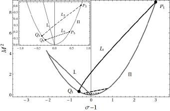
(a) Ground States $n=2$, $p=1$ and descendants

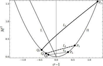
(b) Ground States $n=3$, $p=2$ and descendants

Figure 2: Trajectories in parameter space ($\sigma-1,M^{2}$). (a) States with $n=2$ are represented by the solid curve $L_{1}$ for $R$ in the interval $[1,3]$. This curve originates at the point $P_{1}=(3,9)$ when $R=1$ (geodesic circle) and terminates at the point $Q_{1}=(-5/9,25/81)$ when $R_{3}$ (a triply covered geodesic circle). Both lie on the boundary parabola $\Pi$. The straight line L indicates loops passing through the poles. The descendant states with $n=4$ ($n=6$) which occur for $R$ in the interval $[3,5]$ ($[5,7]$) are represented by the dashed curve $L_{3}$ (dotted curve $L_{5}$) in (a), where they are also shown with zoom in the inset. The counterpart of (a) for the state $n=3$, $p=2$ and its descendants is represented in (b). States with $n=3$ for $R$ in the interval $[2,4]$, as well as the descendants with $n=5$ and $n=7$ for $R$ in the intervals $[4,6]$ and $[6,8]$ respectively, are represented by the solid, dashed, and dotted curves, $L_{2}$,$L_{4}$, $L_{6}$.

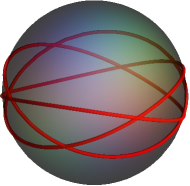
(a) $R=3.05$

(b) $R=4.06$

(c) $R=4.99$

Figure 3: (Color online) States with four-fold symmetry, $n=4$, $p=3$ for $R$ in the interval $[3,5]$: (a) increasingly deformed triple covering of the equator; (b) pole crossing, four points at a time); (c) state making five orbits of sphere before it becomes a quintuple covering of equator. As in Fig. 1 colors represent the normalized local confining force.

In Fig. 4 $\sigma$ and $M^{2}$ are plotted as functions of $R$.

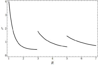
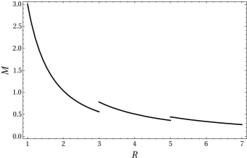
Figure 4: $\sigma$ (a) and $M$ (b) vs. $R$ for $n=2,p=1$ and its descendants in the interval $[1,7]$, as described in the text represented by the trajectories $L_{1},L_{3}$ and $L_{5}$ in Fig. 2. Asymptotically, $\sigma\to 1$ and $M\to 0$.

5.2 Ground state $n=3$, $p=2$ and its descendants

The $n$-fold symmetry states with $p=1$ and their descendants do not exhaust all possible self-intersecting states. If $R=2$, a set of states consisting of a double covering of a geodesic circle ($p=2$) comes into existence with symmetry $n=3,5,7,\dots$. The sequence $L_{2}$ with $n=3$ is illustrated in Fig. 5 for values of $R$ in the interval $[2,4]$. As $R$ is increased, the state with $n=3$ has least energy. As before, one can show that it is the only stable member among these states. It also has a lower energy than its counterpart with $n=2$, and $p=1$ illustrated in Fig. 1.

The trajectory $L_{2}$ representing these states in parameter space as $R$ is varied in the interval $[2,4]$, is represented in Fig. 2(b) by a solid curve. When $R=4$ a transition occurs to a state with a five-fold symmetry. The sequence of trajectories $L_{2},L_{4},L_{6},\dots\,$ is generated. Their endpoints converge to the same point $P_{\infty}=(1,0)$ as those of the sequence $L_{1},L_{3},L_{5},\dots\,.$

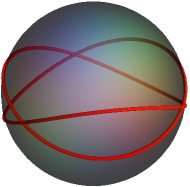
(a) $R=2.05$

(b) $R=2.5$

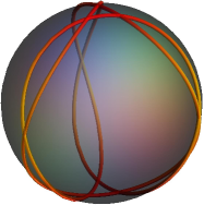
(c) $R=3.0$

(d) $R=3.08$

(e) $R=3.5$

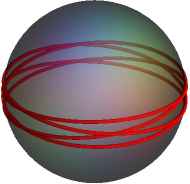
(f) $R=3.99$

Figure 5: (Color online) State with three-fold symmetry for $R$ in the interval $[2,4]$: (a),(b),(c) increasingly deformed double covering of the equator; (d) pole crossing, three points at a time); (e) state making four orbits of sphere; (f) quadruple covering of equator. As in Fig. 1 colors represent the normalized local confining force.

5.3 Loop Energy

The bending energy Eq. (43) can be recast explicitly as a function of $R$:

$$H=\frac{16\,n^{2}}{\pi R}\,{\cal K}[m]\,\left({\cal E}[m]+(m-1){\cal K}[m]\right)+\pi R\,,$$ (58)

where ${\cal E}[m]$ is the complete elliptic integral of the second kind [24], and $m$ is determined by solving Eq. (56).

$H$ is plotted as a function of $R$ for the ground state with $n=2$ and $p=1$ and its descendants in Fig. 6. Expanding expression (58) to second order in $\Delta R=R-1$ we reproduce Eq.(44).

The normal energy, represented by the last term, grows linearly with $R$ and is state independent. In contrast the energy associated with geodesic curvature, represented by the first two terms in Eq.(58), depends sensitively on the state. It is bounded and its maxima fall monotonically as the loop becomes large. It is simple to place a crude upper bound on this falloff: one has $M\approx 2/R$, so that the $H_{g}\leq 2/R$. Thus in a large loop, the geodesic contribution to the energy is negligible compared to its state independent normal counterpart.

The geodesic energy vanishes when $R=1,3,5,\dots$, where the loop collapses to a multiple covering of a geodesic circle. The discontinuities in the derivative of $H$ with respect to $R$ at $R=3,5,\dots$, are directly associated with the change of symmetry at these values of $R$. In the intervals between consecutive values, $H$ increases linearly from zero and rises to a maximum value before falling to zero, again linearly. Behavior is not symmetrical in these intervals. The slopes are different at the two ends and the maximum is not centered. While the maxima are not exactly periodic, they do migrate to the center of their respective intervals as $R$ increases. The existence of these maxima can be understood as a consequence of the incommensurability of the loop with geodesic behavior. The strongly asymmetrical initial maximum is associated with the development of overhangs on the loop before it crosses the poles. As the loop becomes longer this incommensurability plays a diminishing role.

This qualitative behavior is repeated for the odd ground states $n=3$, $p=2$ and its descendants, as well as the excited counterparts of these states. Strikingly, the energy of any closed equilibrium loop tends to a common value in the limit, independent of the state, that completely dominated by the normal energy. The finite gap between the ground state and excited states state disappears.

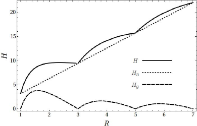
Figure 6: The total energy of the $n=2$ ground state and its descendants as a function of $R$ is represented by a solid curve. It is sum of geodesic and normal parts which are plotted separately as a dashed curve and a dotted line. The normal energy grows linearly and dominates in large loops. By contrast, the geodesic energy is bounded, vanishing at odd integers where its derivative is discontinuous. Its maxima between zeros decrease inversely with $R$.

If $R-1$ is not small, the stability analysis is rather more complicated than the one presented in the context of weak confinement. The results of Ref. [23] in another context implies that, although the details differ, the conclusions for weak confinement continue to hold for values of $R$ before the onset of self-intersection and only the state $n=2,3,4,\dots$, $p=1$ are excited. A detailed analysis of stability has yet to be performed beyond this point. One would, however, expect that the instabilities persist.

The stability of the $n=2$, $p=1$ ground state and its descendants needs to be reassessed when $R\geq 2$. For now one has to accommodate the existence of a set of states described by $n=3,4,5,\dots\,$ $p=2$ and their descendants. In particular, within a finite interval of values of $R$ above $R=2$, the state $n=3$, $p=2$, represented in Fig. 5 has lower energy than the state with $n=2$ and $p=1$ represented in Figure 1). See Fig. 7. The difference in energy is associated with the significant geodesic curvature of the latter when $R\approx 2$. Its descendants with $n=5,7,\dots$ also will have lower energy than their even counterparts when $R\approx 4,6,\dots$.

There are, of course, no smooth deformations taking one from a loop with $p=1$ to one with $p=2$ that remain attached to the sphere. A hairpin costing an infinite bending energy will necessarily always form. However, it is possible to sidestep this topological obstruction by permitting the loop to detach into the interior. While a rigorous stability analysis is beyond the scope of this paper, we will argue that a finite energy barrier will always separate the two surface-bound states. This involves the construction of a natural homotopy connecting these states. Let

$${\bf Y}_{t}=(1-t){\bf Y}_{0}+(1-t){\sf R}(\omega){\bf Y}_{1}\,,$$ (59)

where we represent by ${\bf Y}_{0}$ the initial state with $n=2,p=1$ and by ${\bf Y}_{1}$ the final state with $n=3,p=2$. These interpolating non-equilibrium states will also be confined within the sphere due to the convexity of the latter. The two boundary states have $R=2$. A rotation ${\sf R}(\omega)$ of the final state about the axis of symmetry is introduced in order to initialize the pointwise sum so as to avoid the development of cusps. Intermediates in this homotopic sequence are illustrated in Fig. 8 with the constant choice $\omega=\pi/6$. The bending energy is plotted in Fig. 9 as a function of $t$. It exhibits a finite potential barrier separating the two states. While this does not prove that the $n=2$ state is stable in this regime, it does suggest that it is.

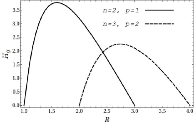
Figure 7: Comparing the geodesic energies of the states with two and three fold symmetries in an interval of $R$ in the neighborhood of $R=2$ (solid and dashed lines respectively). The geodesic energy, and thus the total energy, of the three-fold is lower than that of the two-fold in a finite interval of $R$ beginning at $R=2$.

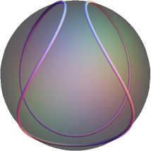
(a) $t=0$

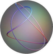
(b) $t=0.2$

(c) $t=0.4$

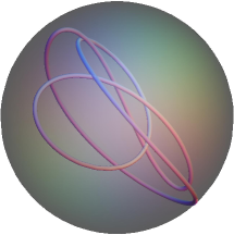
(d) $t=0.6$

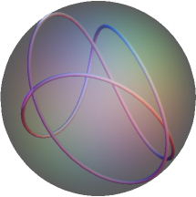
(e) $t=0.8$

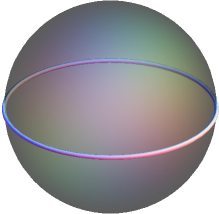
(f) $t=1$

Figure 8: (Color online) Homotopy connecting the two states $n=2,p=1$ and $n=3,p=2$ with $R=2$.

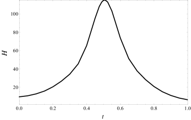
Figure 9: Total energy along a homotopy interpolating between two stable ground states. An energy barrier always exists between the two.

One cannot rule out the existence of semiattached equilibrium states of the loop. We were, however, unable to construct any such states. If they do exist, one would expect them to be unstable.

5.4 Transmitted forces

Using Eq. (51), the local force per unit length transmitted to the sphere is given explicitly as the following function of $s$,

$$\lambda(s)=\frac{1}{2}\kappa^{2}_{g}+\sigma=q^{2}\left(2\,\mbox{dn}^{2}\left(q\,s,m\right)-1\right)\,,$$ (60)

where $\text{dn}^{2}[u,m]=1-m\,\text{sn}^{2}\,[u,m]$ [24]. Whereas the transmitted force depends on the local value of $\kappa_{g}$, both $\kappa_{g}$ and $\sigma$ depend on the boundary conditions associated with closure. Thus $\lambda$ does depend on the global loop geometry. Note that the expansion of the expression in (60) to second order in $\Delta R=R-1$ reproduces the result for weak confinement (Eq. (46)).

In Fig. 10 the maximum and minimum values of $\lambda$ have been plotted as a function of $R$ for the two-fold “ground” state and its descendants. It is positive everywhere with the minimum given by $\sigma$. One observes that $\lambda$ does not behave in a monotonic way, suffering a positive discontinuity whenever $R=p$, where $p$ is an odd integer. This is associated with the transition from orbital to oscillatory behavior at these values and is the analog of the Euler instability described in the discussion of a weakly confined loop. If the unstretchability constraint is relaxed the discontinuity will be smoothed but the jump will persist. Within the individual intervals between discontinuities both the maximum and minimum values decrease monotonically with $R$; this is associated with the reduction in the force once buckling into a state of oscillation has occurred. Curiously, whereas the maxima within these intervals decrease with $R$, the corresponding minima increase. This occurs in such a way that the mean of their values increases monotonically. Both maxima and minima approach the value $\sigma=1$ asymptotically.

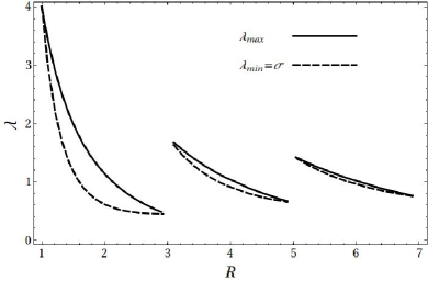
Figure 10: Transmitted force. Maximum (solid line) and minimum (dashed line) values of $\lambda$ as a function of $\Delta R$ in the two-fold ground state with $n=2$, $p=1$, $\lambda$ in the two-fold ground state and its minimum energy descendants.

Recall that the transmitted force is bounded from below by $\sigma$ (see Eq.(45)). Thus, if $\sigma>0$, then $\lambda$ is also; the confined loop will then push on the sphere everywhere. If, however, $\sigma<0$ then $\lambda$ may change sign along the curve. While $\sigma$ is positive in the ground state and its descendants, it may become negative in the excited states of sufficiently long loops. In particular, we find that all states with $n\geq 5$ and $p=1$ exhibit regions in which $\lambda$ turns negative at values of $R$ below the onset of self-contact. When $n=5$ and $p=1$, this occurs when $R\geq 2.536$ (see fig 11(a)). Such states are, however, unstable.

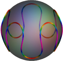
(a) Oscillatory State $n=5$, $p=1$

(b) Orbital State $n=2$, $p=1$

Figure 11: (Color online) (a) The state $n=5$, $p=1$ with $R=2.536$. Above this value of $R$, $\lambda$ may be negative in places. (b) The state $n=2$, $p=1$ with $R=1.85$ inhabits a single hemisphere. These orbital states always have intervals where $\lambda$ is negative.

It may appear counterintuitive that $\lambda$ can be negative. It has to be remembered, however, that while $\lambda$ depends only on the local geometry, this geometry is determined by the global behavior of the loop through the boundary conditions. If one cuts a loop somewhere, the state will immediately relax into a geodesic state with constant positive $\lambda$ everywhere. The existence of regions along the loop where $\lambda<0$ does not necessarily signal a tendency to detach. This will depend on details of the energy landscape.

The states examined here are those consistent with the bound Eq. (23). As was pointed out, states that violate this bound are always unstable with respect to the unbinding of the loop into the interior. Such a state is illustrated in Fig. 11(b), making two self-intersecting orbits in the northern hemisphere. The curvature is high within the two orbits so that this state is evidently an excited state of the loop. The transmitted force $\lambda$ is negative everywhere below the circle with $\kappa_{g}=\sqrt{-2\sigma}$ (see Fig. 11(b)). This suggests that the likely mode of instability will involve the loop unbinding along regions where $\lambda$ is negative, allowing the loop to relax toward the ground state $n=2$, $p=1$ through the unwinding of the high curvature orbits.

Intuitively, one might have expected the total force transmitted to the sphere, $\Lambda=\int ds\lambda$ to increase with loop size. This is not generally the case, except in the limit of large loops, where $\Lambda$ increases linearly with $R$, a consequence of the asymptotic behavior of $\sigma$. Notice also that $\Lambda$ is not the same as the energy $H$ (divided by the radius of the sphere) for finite values of $R$. One has $\Lambda=H-2\pi R(1-c(R))$. In the limit, however, the two do coincide. $\Lambda$ is plotted as a function of $R$ in Fig. 12.

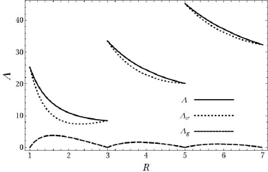
Figure 12: $\Lambda$ vs. $R$ (solid line). The dashed line indicates the contribution from geodesic curvature $\Lambda_{\textit{g}}$. The dotted line is the contribution $\Lambda_{\sigma}=2\pi R\sigma(R)$.

6 Discussion

The confinement of a closed semiflexible loop by a surface has been examined. The constraint on the spatial degrees of freedom of the loop is enforced in the variational principle using the method of Lagrange multipliers. The loss of Euclidean invariance of the energy of the unconstrained loop under confinement is quantified by the Lagrange multiplier which, in equilibrium, gets identified as the force transmitted to the surface by the confined loop.

We have focused on a description of the ground state of a confined loop. If the loop is short this consists of an oscillation about a geodesic circle, exhibiting a two-fold dihedral symmetry. This is the only stable state of the loop in this regime. The description of the ground state and its excitations gets more complicated when the loop length is increased. When $R$ is increased above $2R_{0}$, a new set of states comes into existence that oscillates about a double covering of a geodesic circle. Among these the state with three-fold symmetry has lowest energy; within a finite band of values of $R$, this state also replaces the two-fold as the ground state. The two states remain separated by an energy barrier so that the two-fold remains stable. As the loop size increases these states get replaced by descendants with higher $n$-fold symmetries which alternate as ground states. Both the energy and the transmitted force suffer discontinuities associated with changes of symmetry. They do not generally increase monotonically with loop size except asymptotically. In this limit the energy gap between the ground state and excited states disappears.

Our examination of the confinement of a loop within a spherical cavity might lead one to expect that the equilibrium states of a confined loop will always attach. However, other confining geometries display very different behavior. Consider, for example, the confinement of a loop by a cylinder of smaller radius. Analogs of the $n$-folds exist but, in general, they do not provide the ground state as one can easily verify by playing with metal rings in a wastepaper basket. The details are surprisingly complicated. In this context, it would be interesting to understand how the spherical equilibrium states “evolve” under elliptical deformations of the sphere, or what effect surface irregularities or pores have on the confinement process.

When contact with the confining surface is incomplete, one needs to address the issue of boundary conditions at points of contact. If the contact is due entirely to geometric hindrance, the boundary conditions at isolated points of contact are simple: the tangent vector to the curve is tangent to the surface at these points. If contact extends over a finite region, however, in addition to the tangent vectors the curvatures will also be continuous at the boundary of the region of contact. There may also be a tendency to either promote or inhibit adhesion to the confining surface. A simple way to accommodate such interactions is to introduce a local contact energy, proportional to the length of the contact interval. The boundary conditions will reflect this additional energy. While the curvature will suffer a discontinuity analogous to the discontinuity associated with the contact line bounding the region of contact between a fluid membrane and an attractive substrate [26, 27, 28, 29], this is not the full story. The normals may rotate about the tangent vector, aligning themselves with some preferred direction on the confining geometry. The extension of our framework to accommodate contact energies will be presented elsewhere.

In this paper the role played by the confining surface has been passive: we have not considered the possibility that it may deform in reaction to the presence of the confined polymer. Surface deformations due to membrane bound polymers may also play a role in shaping the morphologies of biological membranes. The forces transmitted to the membrane will now provide a source for the surface stress. Understanding this coupling poses technical challenges. What is clear is that there will be interesting physics associated with the competing elastic energies [30].

Appendix Appendix A Tension in an unconstrained elastic space curve

There are various derivations of Eq. (19). The approach adopted here involves treating the tangent vector to the curve ${\bf T}={\bf Y}^{\prime}$ as an independent variable. If the curve is also parametrized by arc-length, ${\bf T}$ is a unit vector, ${\bf T}^{2}=1$. Thus, consider the energy functional ($\kappa^{2}={\bf T}^{\prime 2}$),

$$H_{1}[{\bf Y},{\bf T},\Lambda,{\bf F}]=\int ds\,\left(\frac{1}{2}\,{\bf T}^{\prime}{}^{2}-\frac{1}{2}\Lambda({\bf T}^{2}-1)+{\bf F}\cdot({\bf T}-{\bf Y}^{\prime})\right)\,;$$ (A.1)

the presence of the two constraints liberates ${\bf T}$ to be varied independently. Now the variation of $H_{1}$ with respect to${\bf Y}$ is given by

$$\delta_{\bf Y}H_{1}=\int ds\,{\bf F}^{\prime}\cdot\delta{\bf Y}\,,$$ (A.2)

whereas its counterpart with respect to ${\bf T}$ is

$$\delta_{\bf T}H_{1}=\int ds\,({\bf F}-{\bf T}^{\prime\prime}-\Lambda\,{\bf T})\cdot\delta{\bf T}\,.$$ (A.3)

Modulo the Frenet-Serret equations for the curve, $\delta_{\bf T}H_{1}=0$ in Eq. (A.3) implies

$${\bf F}=(-\kappa^{2}+\Lambda)\,{\bf T}+\kappa^{\prime}\,{\bf N}+\kappa\tau\,{\bf B}\,.$$ (A.4)

For an isolated elastic curve, ${\bf F}^{\prime}=0$. If the curve is constrained to lie on a surface, it was seen in Sec. 2 that ${\bf F}^{\prime}=\lambda{\bf n}$. Thus the tangential equation ${\bf t}\cdot{\bf F}^{\prime}=0$ continues to hold. This equation can be integrated to determine the Lagrange multiplier $\Lambda$ associated with the parametrization by arclength

$$\Lambda=\frac{3}{2}\kappa^{2}-c\,,$$ (A.5)

where $c$ is a constant of integration. Equation (4) follows.

With respect to the Darboux frame, $\mathbf{F}$ is given by

$$\mathbf{F}=\left(\frac{\kappa_{g}^{2}+\kappa_{n}^{2}}{2}-c\right)\mathbf{T}+\left(\kappa^{\prime}_{n}+\kappa_{g}\tau_{g}\right)\mathbf{n}+\left(\kappa_{g}^{\prime}-\kappa_{n}\tau_{g}\right)\mathbf{l}\,,$$ (A.6)

where we have used the relations (B.4) derived below.

Appendix Appendix B Darboux frame for surface curves

The structure equations (analogous to the Frenet-Serret equations) describing the Darboux frame are given by

$$\mathbf{T}^{\prime} = \kappa_{n}\mathbf{n}+\kappa_{g}\mathbf{l}\,,$$ (B.1a)

$$\mathbf{n}^{\prime} = -\kappa_{n}\mathbf{T}-\tau_{g}{\bf l}\,,$$ (B.1b)

$$\mathbf{l}^{\prime} = -\kappa_{g}{\bf T}+\tau_{g}\mathbf{n}\,.$$ (B.1c)

The normal curvature, the geodesic curvature, and torsion are given, respectively, by

$$\kappa_{n}={\bf T}^{\prime}\cdot{\bf n}=-K_{ab}t^{a}t^{b}\,,\qquad\kappa_{g}={\bf T}^{\prime}\cdot{\bf l}=l^{a}t^{b}\nabla_{b}t_{a}\,,\qquad\tau_{g}={\bf l}^{\prime}\cdot{\bf n}=-K_{ab}t^{a}l^{b}\,.$$ (B.2)

Here $t^{a}$ and $l^{a}$ are the components of the vectors ${\bf T}$ and ${\bf l}$ with respect to a basis of surface tangent vectors adapted to the parametrization, ${\bf e}_{a}$, $a=1,2$: ${\bf T}=t^{a}{\bf e}_{a}$, ${\bf l}=l^{a}{\bf e}_{a}$. $K_{ab}={\bf e}_{a}\cdot\partial_{b}{\bf n}$ is the extrinsic curvature tensor defined on $M$ and $\nabla_{a}$ is the covariant derivative compatible with the induced surface metric $g_{ab}={\bf e}_{a}\cdot{\bf e}_{b}$. Whereas $\kappa_{n}$ and $\tau_{g}$ depend on the extrinsic curvature, $\kappa_{g}$ is defined intrinsically; it depends only on the surface metric $g_{ab}$. The Frenet curvatures are related to their Darboux counterparts by

$$\kappa_{g}=\kappa\,\sin\omega\,,\quad\kappa_{n}=\kappa\,\cos\omega\,,\qquad\tau=\omega^{\prime}-\tau_{g}\,,$$ (B.3)

so that $\kappa^{2}=\kappa_{g}^{2}+\kappa_{n}^{2}$. Thus, the Frenet curvature can be decomposed into its intrinsic and extrinsic parts. The Frenet torsion $\tau$ is the sum of the derivative of the angle connecting both frames and the geodesic torsion. Note that $\tau_{g}$ involves two derivatives, whereas $\tau$ involves three. The extra derivative is associated with $\omega^{\prime}$, the rotation rate of one frame with respect to the other.

The identities Eqs. (B.3) imply the following:

$$\kappa^{\prime}_{g}=\frac{\kappa^{\prime}}{\kappa}\kappa_{g}+\kappa_{n}\left(\tau+\tau_{g}\right)\,,\qquad\kappa^{\prime}_{n}=\frac{\kappa^{\prime}}{\kappa}\kappa_{n}-\kappa_{g}\left(\tau+\tau_{g}\right)\,.$$ (B.4)

These relations are used in Sec. 2 to express the Euler-Lagrange derivatives for the curve in terms of $\kappa_{g}$, $\kappa_{n}$, and $\tau_{g}$ and their derivatives.

Appendix Appendix C Identities for weak spherical confinement

We first derive the relationship between arc-length and the angle $\varphi$ correct to second order. One has

$$s=\int d\varphi\,\left[\left(\frac{d\vartheta}{d\varphi}\right)^{2}+\sin^{2}\vartheta\right]^{1/2}\,.$$ (C.1)

Using Eq. (29) and the harmonic approximation for $\kappa_{g}$ given by Eq. (38), one obtains

$$\sin^{2}{\vartheta}\approx 1-\frac{A_{1}^{2}}{M_{0}^{2}}\cos^{2}n\varphi\,,\qquad\mbox{and}\qquad\frac{d\vartheta}{d\varphi}\approx\frac{1}{M_{0}}\,\frac{d\kappa_{1}}{d\varphi}=\frac{nA_{1}}{M_{0}}\,\sin n\varphi\,.$$ (C.2)

Thus, in this approximation,

$$s\approx\varphi+\frac{1}{4}\frac{A_{1}^{2}}{(n^{2}-1)^{2}}\left((n^{2}-1)\varphi-\frac{\left(n^{2}+1\right)}{2n}\sin 2n\varphi\right)\,.$$ (C.3)

This implies that

$$\Delta R=\frac{1}{4(n^{2}-1)}\,A_{1}^{2}\,.$$ (C.4)

We now derive Eqs. (40) and (41). To do this one needs to examine the boundary conditions (34) and (35) correct to second order in $\epsilon=\sqrt{\Delta R}$. At this order, the turning point $k_{1}$ of the potential $V(\kappa_{g})$, defined by Eq. (25), coincides with $A_{1}$ given in the harmonic approximation by Eq.(39). Thus, the roots in the factorization of $E^{2}-V(\kappa)$ given in Eq. (26), where $E$ is is the constant defined below Eq. (25) are

$$k_{1}^{2}=2(E-\sigma)\approx A^{2}_{1}\,,\qquad K^{2}=2(E+\sigma)\approx-4n^{2}-\frac{2}{n^{2}}(\sigma_{2}-M_{2})-2(\sigma_{2}+M_{2})\,.$$ (C.5)

One thus has, correct to second order,

$$\frac{1}{\sqrt{E^{2}-V(\kappa_{g})}}\approx\frac{1}{n}\frac{1}{\sqrt{A_{1}^{2}-\kappa_{g}^{2}}}\left(1-\frac{1}{4n^{4}}(\sigma_{2}-M_{2})-\frac{1}{4n^{2}}(\sigma_{2}+M_{2})-\frac{1}{8n^{2}}\kappa_{g}^{2}\right)\,.$$ (C.6)

Equation (34) then implies that

$$\Delta R=-\frac{1}{4n^{4}}(\sigma_{2}-M_{2})-\frac{1}{4n^{2}}(\sigma_{2}+M_{2})-\frac{1}{16n^{2}}A_{1}^{2}\,.$$ (C.7)

Furthermore, to second order,

$$M\,\frac{\frac{1}{2}\kappa_{g}^{2}+\sigma-1}{M^{2}-\kappa_{g}^{2}}\approx 1+\frac{1}{n^{2}-1}(\sigma_{2}-M_{2})+\frac{1}{2(n^{2}-1)}\frac{n^{2}+1}{n^{2}-1}\,\kappa_{g}^{2}\,.$$ (C.8)

Equation (35) then implies that for $n\neq 1$,

$$\Delta R=-\frac{1}{n^{2}-1}(\sigma_{2}-M_{2})-\frac{1}{4(n^{2}-1)}\frac{n^{2}+1}{n^{2}-1}\,A_{1}^{2}\,.$$ (C.9)

References

- [1] A. J. Spakowitz and Z. G. Wang, Phys. Rev. Lett. 91, 166102 (2003).
- [2] E. Katzav, M. Adda-Bedia, and A. Boudaoud, Proc. Natl. Acad. Sci. USA 103, 18900 (2006); L. Boué and E. Katzav, Europhys. Lett. 80, 54002 (2007).
- [3] M. Kardar (http://www.mit.edu/kardar/teaching/projects/dna_packing_website/in dex.html).
- [4] K. Ostermeir, K. Alim and E. Frey, Soft Matter 6, 3467 (2010).
- [5] N. Stoop, J. Najafi, F. K. Wittel, M. Habibi and H. J. Herrmann, Phys. Rev. Lett. 106, 214102 (2011).
- [6] R. Levien, University of California at Berkeley, Technical Report No. UCB/EECS-2008-103, 2008.
- [7] J. Langer and D. A. Singer, J. Differenttial Geom. 20, 1 (1984).
- [8] T. A. Ivey and D. A. Singer, Proc. Lond. Math. Soc. 79, 429 (1999).
- [9] D. A. Singer, in Proceedings of Curvature and Variational Modelling in Physics and Biophysics, Edited by O. J. Garay, E. García-Río and R. Vázquez-Lorenzo, (American Institute of Physics, College Park, MD, 2008).
- [10] R. Capovilla, C. Chryssomalakos and J. Guven, J. Phys. A: Math. Gen. 35, 6571 (2002).
- [11] G. S. Manning, Quart. Appl. Math. 45, 515 (1987).
- [12] H. K. Nickerson and G. S. Manning, Geometria Dedicata 27, 127 (1988).
- [13] N. L. Marky and G. S. Manning, Biopolymers 31, 1543 (1991).
- [14] R. Zandi and J. Rudnick, Phys. Rev. E 64, 051918 (2001).
- [15] H. Schiessel, J. Phys.: Condens. Matter 15, R699-R774 (2003).
- [16] G. H. M. Van der Heijden, M. A. Peletier and R. Planqué, Arch. Rat. Mech. Anal. 182, 471 (2006).
- [17] L. Boué, M. Adda-Bedia and A. Boudaoud, in Proceedings of Rencontres du non-linéaire, edited by R. Ribotta (Paris Onze Editions, Orsay, 2006).
- [18] L. D. Landau and E. M. Lifshitz Theory of Elasticity (Butterworth-Heinemann, Oxford, 1999).
- [19] G. Brunnett and P. E. Crouch, Adv. Comput. Math. 2, 23 (1994).
- [20] J. Arroyo, O. J. Garay and J. Mencía J. Phys. A: Math. Gen. 39, 2307 (2006).
- [21] J. Guven and M. M. Müller J. Phys. A: Math. Gen. 41, 055203 (2008).
- [22] J. Guven, M. M. Müller and M. Ben Amar, Phys. Rev. Lett 101, 156104 (2008).
- [23] J. Guven, M. M. Müller and P. Vázquez-Montejo, J. Phys. A: Math. Theor. 45, 015203 (2012).
- [24] M. Abramowitz and I. A. Stegun, Handbook of Mathematical Functions: with Formulas, Graphs, and Mathematical Tables (Dover, New York, 1965).
- [25] N. Stoop, F. K. Wittel, M. B. Amar, M. M. Müller and H. J. Herrmann, Phys. Rev. Lett. 105, 068101 (2010).
- [26] U. Seifert, Adv. Phys. 46, 13 (1997).
- [27] U. Seifert and R. Lipowsky, in Handbook of Biological Physics, edited by R. Lipowsky and E. Sackmann (Elsevier Science, Amsterdam, 1995), Vol. 1.
- [28] R. Capovilla and J. Guven Phys. Rev. E 66, 041604 (2002).
- [29] M. Deserno, M. M. Müller and J. Guven Phys. Rev. E 76, 011605 (2007).
- [30] This point was convincingly illustrated recently in a related context by L. Giomi and M. Mahadevan, e-print arXiv:1108.0597v2.