Crossover from isotropic to directed percolation

Abstract

We generalize the directed percolation (DP) model by relaxing the strict directionality of DP such that propagation can occur in either direction but with anisotropic probabilities. We denote the probabilities as $p_{\downarrow}=p\cdot p_{d}$ and $p_{\uparrow}=p\cdot(1-p_{d})$, with $p$ representing the average occupation probability and $p_{d}$ controlling the anisotropy. The Leath-Alexandrowicz method is used to grow a cluster from an active seed site. We call this model with two main growth directions biased directed percolation (BDP). Standard isotropic percolation (IP) and DP are the two limiting cases of the BDP model, corresponding to $p_{d}=1/2$ and $p_{d}=0,1$ respectively. In this work, besides IP and DP, we also consider the $1/2<p_{d}<1$ region. Extensive Monte Carlo simulations are carried out on the square and the simple-cubic lattices, and the numerical data are analyzed by finite-size scaling. We locate the percolation thresholds of the BDP model for $p_{d}=0.6$ and $0.8$, and determine various critical exponents. These exponents are found to be consistent with those for standard DP. We also determine the renormalization exponent associated with the asymmetric perturbation due to $p_{d}-1/2\neq 0$ near IP, and confirm that such an asymmetric scaling field is relevant at IP.

I Introduction

Directed percolation (DP), introduced in 1957 by Broadbent and Hammersley DP , is a fundamental model in non-equilibrium statistical mechanics and represents the most common dynamic universality class Marro-Dickman . DP has a very wide application, including flow in a porous rock in a gravitational field, forest fires, epidemic spreading, and surface chemical reactions Grassberger-JSP-79-13 . The DP process can be illustrated in the simple example of bond DP on the square lattice. Along the horizontal (vertical) edges of the lattice, the propagation occurs in a particular direction only, e.g., toward the right (the up). Frequently, the preferred spreading direction is termed “temporal,” and the perpendicular one is called “spatial;” the two-dimensional DP is thus often called “(1+1)-dimensional DP.” The DP process has two distinct phases: the inactive phase for small occupation probability $p$ where the propagation quickly dies out, and the active phase for large $p<1$. Between these two phases, a transition occurs at $p_{c}$. As the threshold $p_{c}$ is approached, the temporal ($\parallel$) and the spatial ($\perp$) correlation lengths diverge but with distinct critical exponents: $\xi_{\parallel}\sim|p-p_{c}|^{-\nu_{\parallel}}$ and $\xi_{\perp}\sim|p-p_{c}|^{-\nu_{\perp}}$. The anisotropy is characterized by the so-called dynamic exponent $z=\nu_{\parallel}/\nu_{\perp}$. For $p>p_{c}$, the order parameter ${\mathcal{P}}_{\infty}$, defined as the probability that a randomly selected site can generate an infinite cluster, becomes non-zero and its behavior can be described as ${\mathcal{P}}_{\infty}\sim(p-p_{c})^{\beta}$, with $\beta$ another critical exponent. Below the upper critical dimensionality $(d_{c}+1)$ with $d_{c}=4$, the three independent critical exponents, $\nu_{\parallel}$, $\beta$, and $z$, are sufficient to describe the DP universality class. While analytical results are scarce for DP, even in $(1+1)$ dimensions, approximation techniques like series expansion SE1 ; SE2 ; SE3 ; SE4 ; SE5 and Monte Carlo simulations Grassberger-JPA-1989 ; Grassberger-Zhang ; Lubeck ; Voigt-Ziff have produced fruitful results. Moreover, after a great deal of efforts, experimental realization of the DP process has been achieved Takeuchi ; errotum-Takeuchi ; extension-Takeuchi in nematic liquid crystals, where the DP transition occurs between two turbulent states.

Analogously, standard isotropic percolation (IP) IP is a fundamental model in equilibrium statistical mechanics. IP has attracted extensive research attention both in the physical and the mathematical communities, and the critical behavior is now well understood. Due to the isotropy, there exists only one spatial correlation length, which scales as $\xi\sim|p-p_{c}|^{-\nu}$ near $p_{c}$. Numerous exact results are now available in two dimensions (2D). For bond IP on the square lattice, the self-duality yields the threshold $p_{c}=1/2$ Kesten ; the values of $p_{c}$ are also exactly known for bond and site percolation on several other lattices Ziff-06-0 ; Ziff-06-1 ; Ziff-10-0 , or have been determined to a high precision Feng08 . Thanks to conformal field theory and Coulomb gas theory Cardy ; Smirnov ; Lawler ; Kesten-1987 , the critical exponents $\nu$ and $\beta$ are also exactly known as $\nu=4/3$ and $\beta=5/36$.

Figure 1: (a) State of an edge. (b) A typical cluster in the BDP process. The seed is at site o, and the “infected” sites are denoted as solid dots. Dashed lines represent vacant bonds.

In this work, we introduce a generalized percolation propagation process that contains DP and IP as two special cases. On a given lattice, each edge is assigned to one of the three possible states: occupied by a directed bond along a particular direction, occupied by a directed bond against the particular direction, or unoccupied. This is illustrated in Fig. 1 (a), and the associated probabilities are denoted as $p_{\downarrow}$, $p_{\uparrow}$, and $1-p_{\downarrow}-p_{\uparrow}$, respectively. As a result, the percolation process has two main growth directions. For $p_{\downarrow}=p_{\uparrow}$, the symmetry between the two opposite directions is restored, and the system reduces to standard bond IP. In the limiting case $p_{\downarrow}=0$ or $1$, propagation against or along the particular direction is forbidden, and one has standard DP. We call this percolation model with two main growth directions biased directed percolation (BDP). We note that the BDP model is described by the field-theoretic equation in Frey .

A natural question arises: in between standard DP and IP, what is the nature of phase transition for BDP? For later convenience, we replace parameters $p_{\downarrow}$ and $p_{\uparrow}$ by two new variables as

$$p_{\downarrow}=p\cdot p_{d}\;,\hskip 22.76219ptp_{\uparrow}=p\cdot(1-p_{d})\;.$$ (1)

The parameter $p$ is the average bond-occupation probability (irrespective of the bond direction), and $p_{d}$ accounts for the anisotropy. DP corresponds to $p_{d}=0$ or 1, while $p_{d}=1/2$ is for IP.

In this work, extensive Monte Carlo simulations are carried out for BDP in two and three dimensions. A dimensionless ratio is defined to locate the percolation threshold. The data are analyzed by finite-size scaling, and the critical exponents are determined. The numerical results suggest that the asymmetric perturbation due to $p_{d}-1/2\neq 0$ is relevant near IP, and thus that as long as $p_{d}\neq 1/2$, BDP is in the DP universality class. These results further raise the following questions, remaining to be explored. For IP, is the asymmetric renormalization exponent a “new” critical exponent or related in some way to the known ones like $\nu$ and $\beta$? Particularly, can this “new” exponent be exactly obtained in two dimensions? If so, what is the exact value?

The remainder of this work is organized as follows. Section II introduces the BDP model, the sampled quantities, and the associated scaling behavior. Numerical results are presented in Secs. III and IV. A brief discussion is given in Sec. V.

II Model, sampled quantities, scaling behavior

II.1 Model

We shall describe in details the BDP model on the square lattice. The generalization to higher dimensions is straightforward.

As usual in the study of DP or IP, we view the BDP model as a stochastic growth process, and use the Leath-Alexandrowicz method Leath ; Alex to grow the percolation cluster starting from a seed site. Given the square lattice and the seed “o” in Fig. 1(b), for each of the neighboring edges of site o, a random number is drawn to determine the edge state. If and only if the edge is occupied and the direction originates from the seed o, the neighboring site is activated and belongs to the growing cluster. For instance, in Fig. 1(b), the four neighboring edges of site o are all occupied, but site c remains inactivated because of the “wrong” direction. After all the four neighboring edges have been visited, one continues the growing procedure from the newly added sites. In other words, one grows the percolation cluster shell by shell (the breadth-first scheme). The growth of the cluster continues until the procedure dies out or the maximum distance is reached, which is set at the beginning of the simulation.

II.2 Sampled quantities

In the cluster-growing process, the number of activated sites $N(s)$ is recorded as a function of the shell number $s$. Let us count the shell of site “o” to be the first shell, the configuration in Fig. 1(b) has $N=3,5,6$ for $s=2,3,4$, respectively. Besides $N(s)$, one also records the Euclidean distance $r$ of each activated site to the seed “o” for IP and to the $y$ axis for the anisotropic case. The reason for using different definitions of $r$ is that, for the anisotropic case, the average center of activated sites is expected to move linearly along the preferred direction, as $s$ increases. Accordingly, we define a revised gyration radius $R(s)$ as

$$R(s)=\left\{\begin{array}[]{ll}0&\hskip 28.45274pt\mbox{if }N(s)=0\\ \sqrt{\sum_{i=1}^{N}r_{i}^{2}/N}&\hskip 28.45274pt\mbox{if }N(s)\geq 1\\ \end{array}\right.$$ (2)

The statistical averages ${\mathcal{N}}(s)\equiv\langle N(s)\rangle$ and ${\mathcal{R}}(s)\equiv\langle R(s)\rangle$ are then measured, as well as their statistical uncertainties. We also measure the survival probability ${\mathcal{P}}(s)$ that at least one site remains activated at the $s$th shell and the accumulated activated site number ${\mathcal{A}}(s)\equiv\langle\sum_{s^{\prime}=1}^{s}N(s^{\prime})\rangle$.

In Monte Carlo study of critical phenomena and phase transitions, it is found that dimensionless ratios like the Binder cumulant are very useful in locating the critical point. Therefore, we also define a dimensionless ratio $Q_{{\mathcal{N}}}(s)={\mathcal{N}}(2s)/{\mathcal{N}}(s)$.

II.3 Scaling behavior

Near the percolation threshold $p_{c}$, one expects the following scaling behavior

$${\mathcal{P}}(s,\epsilon) \sim s^{-Y_{P}}\mathbb{P}(\epsilon s^{Y_{\epsilon}})\;,$$

$${\mathcal{N}}(s,\epsilon) \sim s^{Y_{N}}\mathbb{N}(\epsilon s^{Y_{\epsilon}})\;,$$

$${\mathcal{A}}(s,\epsilon) \sim s^{Y_{A}}\mathbb{A}(\epsilon s^{Y_{\epsilon}})\;,$$

$${\mathcal{R}}(s,\epsilon) \sim s^{Y_{R}}\mathbb{R}(\epsilon s^{Y_{\epsilon}})\;,$$

$$Q_{{\mathcal{N}}}(s,\epsilon) \sim 2^{Y_{N}}\mathbb{Q}(\epsilon s^{Y_{\epsilon}})\;,$$ (3)

where $\epsilon=p-p_{c}$ represents a small deviation from $p_{c}$. Symbols $Y_{P},Y_{N},Y_{A},Y_{R}$, and $Y_{\epsilon}$ denote the associated critical exponents, and $\mathbb{P},\mathbb{N},\mathbb{A}$, $\mathbb{R}$, and $\mathbb{Q}$ are universal functions. For simplicity, only one scaling field, which accounts for the effect due to deviation from $p_{c}$, is explicitly included in Eq. (3). Right at $p_{c}$, as $s$ increases, the survival probability ${\mathcal{P}}(s)$ decays to zero while the other quantities diverge, except for the ratio $Q_{\mathcal{N}}$ which goes to a constant. A trivial relation is $Y_{A}=Y_{N}+1$.

For standard DP ($p_{d}=0$ or 1), exponents $Y_{P}$ and $Y_{N}$ are normally denoted as $\delta$ and $\eta$, respectively ($Y_{N}$ is also denoted as $\theta$ in Hinrichsen-2000 ). It can be shown that exponent $Y_{\epsilon}$ is $Y_{\epsilon}=1/\nu_{\parallel}$. Further, exponent $Y_{R}$ relates to $\delta$ and the dynamic exponent $z$ as $Y_{R}=-\delta+1/z$, where $-\delta$ arises from the behavior ${\mathcal{P}}(s)\sim s^{-\delta}$. Below the upper critical dimensionality $(d_{c}+1)$ with $d_{c}=4$, there exist three independent exponents, which can be chosen as $\nu_{\parallel}$, $\beta$, and $z$. The others can be obtained by the scaling relations Hinrichsen-2000

$$\nu_{\perp}=\nu_{\parallel}/z\;,\hskip 14.22636pt\delta=\beta/\nu_{\parallel}\;,\hskip 14.22636pt\eta=(d\nu_{\perp}-2\beta)/\nu_{\parallel}\;,$$ (4)

where the last one involves the spatial dimensionality $d$ and is called the hyperscaling relation. In $(1+1)$ dimensions, these exponents have been determined to high precision: $\nu_{\parallel}=1.733\,847(6)$, $\beta=0.276\,486(8)$, and $z=1.580745(10)$ SE4 . In $(2+1)$ dimensions, these exponents are $\nu_{\parallel}=1.2890(7)$, $\beta=0.581\,2(6)$, and $z=1.7665(4)$ Grassberger-Zhang ; Voigt-Ziff ; Perlsman ; Junfeng .

For standard IP ($p_{d}=1/2$), the shell number $s$ is frequently called “chemical distance” Havlin , accounting for the minimum length among all the possible paths between the seed site and the activated sites on the $s$th shell. At $p_{c}$, the length $s$ of the chemical path relates to the Euclidean distance $r$ as $s\sim r^{d_{\rm min}}$ Grassberger-JPA-1992 ; Grassberger-JPA-1985 , with $d_{\rm min}\geq 1$ denoting the shortest-path exponent. In terms of the Euclidean distance $r$, it is known that the survival probability scales as ${\mathcal{P}}(r)\sim r^{-\beta/\nu}$, the accumulated site number ${\mathcal{A}}(r)\sim r^{\gamma/\nu}$, and the $p_{c}$-deviating scaling behavior $\epsilon r^{1/\nu}$. This immediately yields $Y_{P}=-\beta/(\nu d_{\rm min}),Y_{A}=\gamma/(\nu d_{\rm min}),Y_{N}=\gamma/(\nu d_{\rm min})-1,Y_{R}=(1-\beta/\nu)/d_{\rm min}$, and $Y_{\epsilon}=1/(\nu d_{\rm min})$. For IP, one has the scaling relation as

$$\gamma/\nu=d-2\beta/\nu\;.$$ (5)

In 2D, $\nu$ and $\beta$ are exactly known as $\nu=4/3$ and $\beta=5/36$, which yield $\gamma/\nu=43/24\approx 1.79166\ldots$ and $\beta/\nu=5/48\approx 0.104166\ldots$. The shortest-path exponent $d_{\rm min}$, together with the so-called backbone exponent, is among the few critical exponents of which the exact values are not known for the 2D percolation universality class. It was conjectured to be $d_{\rm min}=217/192=1.13020\ldots$ Deng-PRE-81 , and some recent estimates are 1.1306(3) Grassberger-JPA-32 and 1.13078(5) JY . In three dimensions, no exact results are available, and the numerical estimates are $d_{\rm min}=1.374(4)$ Grassberger-JPA-25 , $\beta/\nu=0.4774(1)$ and $\nu=0.8734(6)$ deng , which yield $\beta=0.4170(4)$.

III Results

In this work, we consider the BDP model on the square lattice for 2D and the simple-cubic lattice for 3D. The simulation applies the aforementioned Leath-Alexandrowicz growth method. The dimensionless ratio $Q_{\mathcal{N}}$ is used to locate the percolation threshold $p_{c}$. According to Eq. (3), ratio $Q_{\mathcal{N}}$ is expected to have an approximate common intersection at $p_{c}$ for different shell number $s$. At the threshold $p_{c}$, as $s\rightarrow\infty$, the common intersection converges to a universal value $2^{Y_{N}}$ and the slope of $Q_{\mathcal{N}}$ increases as $s^{Y_{\epsilon}}$.

III.1 Standard IP

Standard IP corresponds to $p_{d}=1/2$. Monte Carlo simulation was carried out up to $s_{\rm max}=8192$ for 2D and $2048$ for 3D. About $10^{8}$ samples were taken for each data point on each lattice. The $Q_{\mathcal{N}}$ data are shown in Fig. 2. Indeed, we find an approximate common intersection near $p=1$ and $0.4976$ for 2D and 3D, respectively. This agrees with the known threshold $p_{c}/2=1/2\;(2D)$ and $0.248\,812\,6(5)\;(3D)$ Lorenz . Note that, since the occupied bond can propagate the growth process only if it has the correct orientation, there is a factor of 2 difference between the bond-occupation probability $p$ here and the $p$ of the equivalent bond percolation probability.

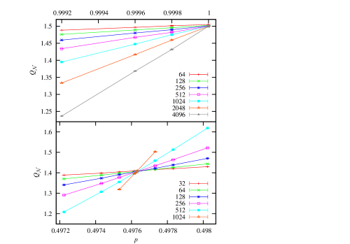
Figure 2: Ratio $Q_{\mathcal{N}}$ for IP in 2D (top) and 3D (bottom).

To have a better estimate of $p_{c}$, according to a least-squared criterion, the $Q_{\mathcal{N}}$ data are fitted by

$$Q_{\mathcal{N}}(s,\epsilon)=Q_{{\mathcal{N}},c}+\sum_{k=1}^{4}q_{k}\epsilon^{k}s^{kY_{\epsilon}}+b_{1}s^{y_{1}}$$

$$+b_{2}s^{-2}+c\epsilon s^{Y_{\epsilon}+y_{1}}+n\epsilon^{2}s^{Y_{\epsilon}}+...\;,$$ (6)

which is obtained by Taylor-expanding Eq. (3) and taking into account finite-size corrections due to the leading irrelevant scaling field and analytical background contribution. These are described by the two terms with amplitudes $b_{1}$ and $b_{2}$, of which the term with $n$ arises from the nonlinearity of the relevant scaling field in terms of the deviation $\epsilon$, and the one with $c$ accounts for the combined effect of the leading relevant and irrelevant scaling fields. In the fits, various formulas are tried, which correspond to different combinations of those terms in Eq. (6). For a given formula, the $Q_{\mathcal{N}}$ data for small $s<s_{\rm min}$ are gradually excluded from the fits to see how the residual $\chi^{2}$ changes with respect to $s_{\rm min}$. The results from different formulas are compared with each other to estimate the possible systematic errors. In two dimensions, we obtain $p_{c}=1.000\,000(4)$, $Q_{{\mathcal{N}},c}=1.499\,5(1)$, $Y_{\epsilon}=0.664(3)$, and $y_{1}=-0.96(6)$. Note that the leading irrelevant thermal scaling field is $\omega=-2$ for 2D percolation universality Ziff-PRE-2011 ; apparently, the leading correction exponent $y_{1}=-0.96$ does not correspond to $\omega$. Instead, $y_{1}$ should be associated with the chemical distance. From the relations $Q_{{\mathcal{N}},c}=2^{Y_{N}}$, $Y_{N}=\gamma/(\nu d_{\rm min})-1$, and $Y_{\epsilon}=1/(\nu d_{\rm min})$, and the exact values $\gamma/\nu=43/24$ and $1/\nu=3/4$, we determine $d_{\rm min}=1.130\,76(10)$ from $Q_{{\mathcal{N}},c}=1.499\,5(1)$, and $d_{\rm min}=1.130(6)$ from $Y_{\epsilon}=0.664(3)$.

In three dimensions, our results are $p_{c}=0.497\,624(1)$, $Q_{{\mathcal{N}},c}=1.400(1)$, $Y_{\epsilon}=0.830(1)$, and $y_{1}=-0.8(2)$. Our estimate of $p_{c}/2=0.248\,812\,0(5)$ agrees with the existing one $0.248\,812\,6(5)$ Lorenz , and has a comparable error margin.

		$\beta$	$\nu$	$d_{\rm min}$	$p_{c}/2$
$2D$	(known)	$5/36$ IP ; Cardy ; Smirnov ; Lawler ; Kesten-1987	$4/3$ IP ; Cardy ; Smirnov ; Lawler ; Kesten-1987	$1.130\,6(3)$  Grassberger-JPA-32 ; Deng-PRE-81 ; JY	$1/2$ IP ; Kesten
	(present)	$0.138\,7(10)$	$1.332(6)$	$1.130\,76(10)$	$0.500\,000(2)$
$3D$	(known)	$0.4167(4)$	$0.873\,4(6)$ deng	$1.374(4)$ Grassberger-JPA-25	$0.248\,812\,6(5)$ Lorenz
	(present)	$0.417(1)$	$0.876(2)$	$1.375(1)$	$0.248\,812\,0(5)$

Table 1: Percolation thresholds and critical exponents for IP.

To estimate other critical exponents, we simulate right at the threshold $p/2=1/2$ for 2D and $0.248\,812\,0$ for 3D. The simulation was carried out for $s$ up to $s_{\rm max}=8192$ for 2D and 2048 for 3D. Further, to eliminate one more unknown parameter in the fits, we measure the dimensionless ratios $Q_{\mathcal{P}}(s)={\mathcal{P}}(2s)/{\mathcal{P}}(s)$ and $Q_{\mathcal{R}}={\mathcal{R}}(2s)/{\mathcal{R}}(s)$. These $Q$ data are fitted by

$$Q(s)=Q_{c}+b_{1}s^{y_{1}}+b_{2}s^{-2}\;.$$ (7)

In two dimensions, the results are $Q_{{\mathcal{P}},c}=0.9382(1)$ and $y_{1}=-0.80(7)$ for $Q_{\mathcal{P}}$, and $Q_{{\mathcal{R}},c}=1.7318(2)$ and $y_{1}=-0.9(1)$ for $Q_{\mathcal{R}}$. For all these three ratios, the leading correction is described by an exponent $y_{1}\approx-1$. Taking into account the exact values $\beta/\nu=5/48$, one has $d_{\rm min}=1.132(2)$ from $Q_{{\mathcal{P}},c}$ and $d_{\rm min}=1.130\,7(3)$ from $Q_{{\mathcal{R}},c}$.

In three dimensions, the results are $Q_{{\mathcal{P}},c}=0.7865(2)$ and $y_{1}=-0.7(2)$ for $Q_{\mathcal{P}}$, and $Q_{{\mathcal{R}},c}=1.3020(3)$ and $y_{1}=-0.9(2)$ for $Q_{\mathcal{R}}$. Combining the estimate $Q_{{\mathcal{P}},c}$ and $Q_{{\mathcal{R}},c}$ together, one has $\beta/\nu=0.4765(8)$ and $d_{\rm min}=1.375(1)$. Our result $d_{\rm min}=1.375(1)$ agrees well with the existing result $d_{\rm min}=1.374(4)$ Grassberger-JPA-25 , and significantly improves the error margin.

For comparison, these results are summarized in Table 1.

III.2 Standard DP

We simulate standard DP by taking $p_{d}=1$. The simulation was carried out for $s$ up to $s_{\rm max}=16384$ for 2D, and 2048 for 3D. The number of samples for each data point is about $8\times 10^{8}$ in 2D and $1.6\times 10^{8}$ in 3D.

The $Q_{\mathcal{N}}$ data are shown in Fig. 3. A good intersection is observed for both 2D and 3D, which yields $p_{c}=0.64470$ for 2D and $0.38222$ for 3D, from a rough visual fitting.

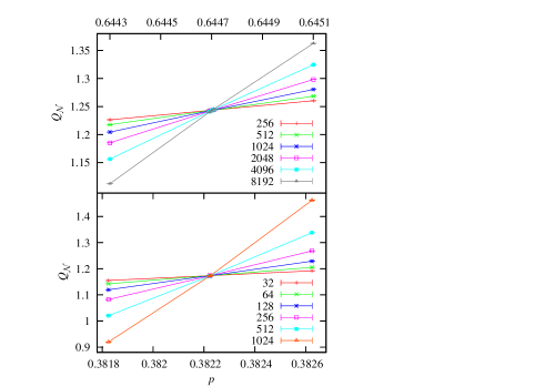
Figure 3: Ratio $Q_{\mathcal{N}}$ for standard DP in 2D (top) and 3D (bottom).

We fit the $Q_{\mathcal{N}}$ data more precisely using Eq. (6). On the square lattice, we obtain $p_{c}=0.644\,700\,5(8)$, $Q_{{\mathcal{N}},c}=1.242\,9(2)$, $Y_{\epsilon}=0.576(3)$, and $y_{1}=-0.9(1)$. The estimate of the percolation threshold agrees well with the existing more precise result $0.644\,700\,185(5)$ SE4 . From the relations $Q_{{\mathcal{N}},c}=2^{Y_{N}}=2^{\eta}$ and $Y_{\epsilon}=1/\nu_{\parallel}$, we have $\eta=0.313\,7(2)$ and $\nu_{\parallel}=1.736(9)$. On the simple-cubic lattice, our results are $p_{c}=0.382\,225\,6(5)$, $Y_{\epsilon}=0.777(2)$, $Q_{{\mathcal{N}},c}=1.1738(1)$, which yield $\eta=0.2312(1)$ and $\nu_{\parallel}=1.287(4)$. Here the $y_{1}$ is too small to estimate since the numerical data of $s\geq 24$ can be well described even though we do not include any corrections. The agreement of $p_{c}$ with the existing estimate $p_{c}=0.382\,224\,64(4)$ Junfeng is within two standard deviations.

Analogously, we simulate right at the percolation threshold $p_{c}=0.644\,700\,185$ for 2D and $p_{c}=0.382\,224\,64$ for 3D. The dimensionless ratios $Q_{\mathcal{P}}$ and $Q_{\mathcal{R}}$ are measured, and the data are fitted by Eq. (7). For 2D, the results are $Q_{{\mathcal{P}},c}=0.89537(5)$, $y_{1}=-0.98(5)$ and $Q_{{\mathcal{R}},c}=1.3882(1)$, $y_{1}=-1.1(1)$, which yield $Y_{P}=\delta=0.159\,44(9)$ and $Y_{R}=(-\delta+1/z)=0.47322(10)$. Taking into account the estimates of $\nu_{\parallel}$ and $\delta$, one has $\nu_{\perp}=1.098(6)$. For 3D, the results are $Q_{{\mathcal{P}},c}=0.7311(4)$ and $Q_{{\mathcal{R}},c}=1.0822(1)$, which yield that $\delta=0.4519(8)$ and $\nu_{\perp}=0.728(4)$.

These results are listed in Table 2.

III.3 BDP

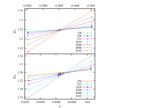
Figure 4: Ratio $Q_{\mathcal{N}}$ for BDP in 2D. The top (bottom) panel corresponds to $p_{d}=0.8$ ($0.6$) case.

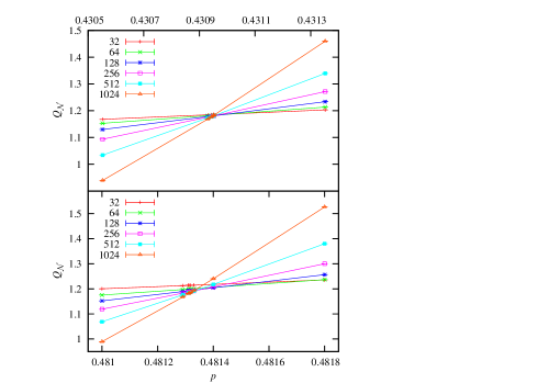
Figure 5: Ratio $Q_{\mathcal{N}}$ for BDP in 3D. The top (bottom) panel corresponds to $p_{d}=0.8$ ($0.6$) case.

For the purpose of studying BDP, we choose $p_{d}=0.6$ and $0.8$. The simulation was carried out for $s$ up to $s_{\rm max}=16384$ for 2D and 2048 for 3D. About $2\times 10^{8}$ samples were taken for each data point in each case.

The $Q_{\mathcal{N}}$ data are shown in Fig. 4 for 2D and Fig. 5 for 3D. The transitions are also clearly observed, but the approximate common intersections are not as good as those for standard DP and IP. This suggests the existence of additional finite-size corrections.

The $Q_{\mathcal{N}}$ data are also fitted by Eq. (6) according to a least-squared criterion. To account for the possible existence of additional corrections, we replace the terms in Eq. (6), with $b_{1}$, $b_{2}$, and $c$, by $b_{i}s^{y_{i}}+b_{1}s^{y_{1}}+c\epsilon s^{y_{i}+y_{\epsilon}}$. The exponent $y_{1}$ is fixed at $-1$, in accordance with our above estimate of $y_{1}$ for both standard IP and DP. Indeed, the new source of finite-size correction can be identified in the fits, which yield $y_{i}=-0.5(2)$ both in 2D and 3D. The results for $p_{c}$, $\eta=\log_{2}Q_{{\mathcal{N}},c}$, and $\nu_{\parallel}=1/Y_{\epsilon}$ are summarized in Table 2.

D	Ref.	$p_{d}$	$p_{c}$	$\beta$	$\nu_{\parallel}$	$z$	$\eta$	$\delta$
2	SE4	1	$0.644\,700\,185(5)$	$0.276\,486(8)$	$1.733\,847(6)$	$1.580\,745(10)$	$0.313\,686(8)$	$0.159\,464(6)$
		1	0.644 700 5(8)	0.277(2)	1.736(9)	1.580 6(3)	0.313 7(2)	0.159 44(9)
		0.8	0.768 708(1)	0.278(2)	1.74(1)	1.577(5)	0.314 1(4)	0.159 5(1)
		0.6	0.929 668(3)	0.279(2)	1.754(6)	1.578(5)	0.316 1(8)	0.159(1)
3	Junfeng	1	0.382 224 64(4)	0.581 2(6)	1.289 0(7)	1.766 5(2)	0.230 81(7)	0.450 9(2)
		1	0.382 225 6(5)	0.582(5)	1.287(4)	1.767(3)	0.231 2(1)	0.451 9(8)
		0.8	0.430 941(2)	0.577(5)	1.289(5)	1.77(1)	0.229(3)	0.448(2)
		0.6	0.481 310(2)	0.583(8)	1.292(5)	1.76(2)	0.226(9)	0.452(4)

Table 2: Percolation thresholds and critical exponents for standard DP ($p_{d}=1$) and BDP ($p_{d}<1$). The numbers in the row with reference are the existing results. Clearly, standard DP and BDP with $p_{d}=0.8,0.6$ share the same critical exponents.

The determination of the critical exponents $\delta$ and $z$ is obtained in an analogous way by simulating at the estimated percolation threshold, and the results are listed in Table 2.

The results in Table 2 strongly suggest that, as long as $p_{d}$ deviates from $1/2$, the system falls into the standard DP universality class. For an illustration, we make the log-log plot of the critical quantity ${\mathcal{N}}$ versus the shell number $s$ in Fig. 6. Clearly, the slope for $p_{d}=1/2$ is distinct from those for the other cases, which are independent of $p_{d}$.

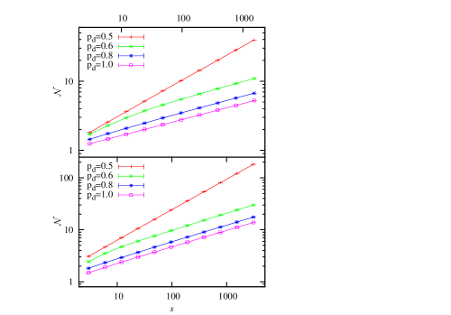
Figure 6: Log-log plot of ${\mathcal{N}}$ versus $s$ at $p_{c}$. The bottom (top) panel is for 2D (3D). It is clearly seen that the slope is identical for all the $p_{d}\neq 1/2$ cases, and is distinct from that of IP ($p_{d}=1/2$).

IV Crossover exponent

The fact that BDP for $p_{d}\neq 1/2$ is in the DP universality means that in the language of renormalization group theory, the operator associated with the asymmetric perturbation is relevant near the IP fixed point. To confirm this, we simulate BDP near IP with $p=p_{c}=1$ by varying $\epsilon_{d}=p_{d}-1/2$. The simulation is up to $s_{\rm max}=8192$, and $\epsilon_{d}$ is set at $0$, $10^{-3}$ and $2\times 10^{-3}$. The results for $Q_{{\mathcal{N}}}$ in two dimensions are shown in Fig. 7 versus $\epsilon_{d}^{2}$; note that BDPs for $\pm\epsilon_{d}$ are identical. These $Q_{{\mathcal{N}}}$ data are also analyzed by Eq. (6) with $Y_{\epsilon}$ being replaced by the exponent $Y_{\epsilon_{d}}$ for the symmetric scaling field and the odd terms with respect to $\epsilon_{d}$ being set zero. We obtain $Y_{\epsilon_{d}}=0.500(5)$, which suggests that $Y_{\epsilon_{d}}$ may be exactly $1/2$.

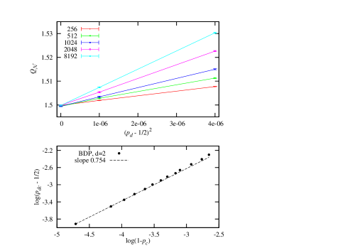
Figure 7: Top: Ratio $Q_{{\mathcal{N}}}$ versus $(p_{d}-1/2)^{2}$ with $p=1$ on square lattice. Bottom: Log-log plot of $p_{dc}-1/2$ versus $1-p_{c}$ for the transition line $(p_{dc},p_{c})$ near IP. The dashed line has slope $0.754$.

According to scaling theory, the phase transition line $(p_{c},p_{dc})$ approaches to the critical IP $(p_{c}=1,p_{dc}=1/2)$ as Riedel-1969

$$1-p_{c}\propto|(p_{dc}-1/2)|^{1/\phi}\;,$$ (8)

where $\phi=Y_{\epsilon_{d}}/Y_{\epsilon}$ is the so-called crossover exponent. We carried out some Monte Carlo simulations and determined a set of critical points near IP; they are 13 critical points with $p_{dc}\in[0.52,0.6]$. In Fig. 7, we plot $p_{dc}-1/2$ versus $1-p_{c}$ in log-log scale, which indeed has slope approximately equal to $\phi=Y_{\epsilon_{d}}/Y_{\epsilon}=0.754$.

We also perform a similar study near the critical IP in 3D, and obtain $Y_{\epsilon_{d}}=0.56(1)$ and $\phi=0.67(1)$.

V Discussion

We introduce a biased directed percolation model, which includes standard isotropic and directed percolation as two special cases. Large-scale Monte Carlo simulations are carried out in two and three dimensions. We find that the operator associated with the anisotropy is relevant near the IP fixed point, which implies that BDP in the region $p_{d}\neq 1/2$ is in the DP university class. On this basis, the phase diagram and the associated renormalization flows are shown in Fig. 8.

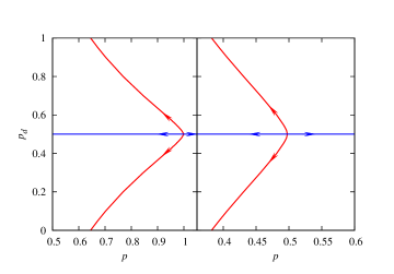
Figure 8: Phase diagram of the BDP model in 2D (left) and 3D (right). The $p_{d}=1/2$ line corresponds to isotropic percolation. The diagram for $p_{d}<1/2$ is drawn by symmetry. The arrows represent the direction of the renormalization flows.

Since the upper critical dimensionality is different for standard IP and DP, it is not clear whether the similar renormalization flows would hold in higher dimensions. We mention that such crossover phenomena have attract much attention both in the fields of equilibrium and non-equilibrium statistical mechanics Pfeuty ; Aharony ; Lubeck-JSM ; Mendes ; Frojdh ; Janssen ; Schonmann-JSP-1986 . In retrospect, it is not surprising that the asymmetric perturbation is relevant near IP. At IP, all the directions are equivalent and “spatial” and “temporal” directions cannot be defined. However, as soon as $p_{d}-1/2\neq 0$, such a symmetry is broken and the center of the activated sites moves along the “temporal” direction as the growing process continues. It is also plausible that as long as the “spatial” and “temporal” symmetry is not restored, such an asymmetric perturbation is irrelevant near DP. This is similar to the fact that asymmetric diffusion on the basic contact process is irrelevant Schonmann-JSP-1986 . In terms of the chemical distance $s$, the effect from the anisotropy can be asymptotically described as $\propto(p_{d}-1/2)s^{Y_{\epsilon_{d}}}$ with $Y_{\epsilon_{d}}(2D)=0.500(5)$ and $Y_{\epsilon_{d}}(3D)=0.589(10)$. One can also use the Euclidean distance $r$ to describe such an anisotropic effect as $\propto(p_{d}-1/2)r^{1/\nu_{d}}$ with $Y_{\epsilon_{d}}=1/(\nu_{d}d_{\rm min})$. Substituting the $d_{\rm min}$ value into $Y_{\epsilon_{d}}$, one obtains $\nu_{d}(2D)=1.77(1)$ and $\nu_{d}(3D)=1.30(2)$.

When viewing standard isotropic percolation in the framework of BDP, one observes that two independent critical exponents, e.g., $\nu$ and $\beta$, are no longer sufficient to describe the critical scaling behavior. In this case, the shortest-path exponent $d_{\rm min}$ appears naturally and becomes indispensable, and thus isotropic percolation also has three independent critical exponents. Our estimate of $d_{\rm min}$ significantly improves over the existing results both in two and three dimensions. Our result $d_{\rm min}=1.130\,76(10)$ does not agree with the recently conjectured value $217/192$ Deng-PRE-81 in two dimensions. This result appears to refute the conjectured value. On the other hand, we note that, in terms of the chemical distance $s$, a new source of finite-size corrections occurs in the scaling behavior, and these corrections are not well understood yet. Further, we observe that the restored symmetry for IP can be regarded as $\nu_{\parallel}=\nu_{\perp}$ in the BDP model. In some cases, the coincidence of two critical exponents may suggest the existence of logarithmic corrections of the $\log$ or $\log\log$ form, and they can be either additive or multiplicative. In practice, logarithmic finite-size corrections have indeed been observed for standard isotropic percolation in two dimensions Feng08 , which is in terms of Euclidean distance. In this sense, we cannot entirely exclude the possibility that the tiny difference between the present numerical result for $d_{\mathrm{min}}$ and the conjectured value arises from some unknown corrections that have not been taken into account in the numerical analysis. Numerical investigation of this problem seems very difficult if not impossible. Nevertheless, since the exact value of $d_{\rm min}$ is conjectured as a function of $q$ for the $q$-state Potts model  Deng-PRE-81 , one can accumulate more numerical evidence by studying the $q\neq 1$ case.

Finally, the numerical estimate of the critical exponent $Y_{\epsilon_{d}}$ or $\nu_{d}$ due to the asymmetric perturbation near IP raises a question: is it a “new” independent critical exponent or simply related in some way to the known ones like $\beta$, $\nu$, and $d_{\rm min}$? In particular, in two dimensions, one would ask whether $\nu_{d}$ or $Y_{\epsilon_{d}}$ can be exactly obtained in the framework of Stochastic Loewner Evolution (SLE), conformal field theory or Coulomb gas theory.

VI Acknowledgments

This work was supported in part by NSFC under Grant No. 10975127 and 91024026, and the Chinese Academy of Science. RMZ acknowledges support from National Science Foundation Grant No. DMS-0553487. We also would like to thank Dr. Timothy M. Garoni in Monash University for valuable comments.

References

- (1) S. R. Broadbent and J. M. Hammersley, Proc. Camb. Phil. Soc. 53, 629 (1957).
- (2) J. Marro and R. Dickman, Nonequilibrium phase transitions in lattice models, Cambridge University Press, Cambridge, 1999.
- (3) P. Grassberger, J. Stat. Phys. 79, 13 (1995).
- (4) K. De’Bell, and J. W. Essam, J. Phys. A 16, 3553 (1983).
- (5) J. W. Essam, K. De’Bell, J. Adler, F. M. Bhatti, Phys. Rev. B 33, 1982 (1986).
- (6) R. J. Baxter and A. J. Guttmann, J. Phys. A 21, 3193 (1988).
- (7) I. Jensen, J. Phys. A 32, 5233 (1999).
- (8) I. Jensen, J. Phys. A 37, 6899 (2004).
- (9) P. Grassberger, J. Phys. A 22, 3673 (1989).
- (10) P. Grassberger and Y. C. Zhang, Physica A 224, 169 (1996).
- (11) C. A. Voigt and R. M. Ziff, Phy. Rev. E 56, R6241 (1997).
- (12) S. Lübeck and R. D. Willmam, J. Stat. Phys, 115, 516 (2004).
- (13) K. A. Takeuchi, M. Kuroda, H. Chatè and M. Sano, Phys. Rev. Lett. 99, 234503 (2007).
- (14) K. A. Takeuchi, M. Kuroda, H. Chatè and M. Sano, Phys. Rev. Lett. 103, 089901 (E) (2009).
- (15) K. A. Takeuchi, M. Kuroda, H. Chatè and M. Sano, Phys. Rev. E 80, 051116 (2009).
- (16) D. Stauffer and A. Aharony, Introduction to Percolation Theory (Taylor and Francis, London, 1992), and references therein.
- (17) H. Kesten, Comm. Math. Phys. 74, 41 (1980).
- (18) R. M. Ziff, Phys. Rev. E 73, 016134 (2006).
- (19) R. M. Ziff and C. R. Scullard, J. Phys. A 39, 15083 (2006).
- (20) C. R. Scullard and R. M. Ziff, J. Stat. Mech. P03021 (2010).
- (21) X. Feng, Y. Deng and H. W. J. Blöte, Phys. Rev. E 78, 031136 (2008).
- (22) J. L. Cardy, Nucl. Phys. B 240, 514 (1984).
- (23) S. Smirnov, W. Werner, Math. Research Letters, 8, 729 (2001).
- (24) G. F. Lawler, O. Schramm, W. Werner, One-arm exponent for critical 2D percolation. Electron. J. Probab. 7, paper no.2 (2002).
- (25) H. Kesten, Comm. Math. Phys. 109, 109 (1987).
- (26) E. Frey, U. C. Taüber, F. Schwabl, Phys. Rev. E 49, 5058 (1994).
- (27) P. L. Leath, Phys. Rev. B 14, 5046 (1976).
- (28) Z. Alexandrowicz, Phys. Lett. A 80, 284 (1980).
- (29) H. Hinrichsen, Adv. Phys. 49, 815 (2000).
- (30) E. Perlsman and S. Havlin, Europhys. Lett. 58, 176 (2002).
- (31) J. Wang, Q. Liu and Y. Deng, arXiv:1201.3006.
- (32) S. Havlin, B. Trus, G. H. Weiss and D. ben-Avraham, J. Phys. A 18, L247 (1985).
- (33) P. Grassberger, J. Phys. A 25, 5475 (1992).
- (34) P. Grassberger, J. Phys. A 18, L215 (1985).
- (35) Y. Deng, W. Zhang, T. M. Garoni, A. D. Sokal, and A. Sportiello, Phys. Rev. E 81, 020102(R) (2010).
- (36) P. Grassberger, J. Phys. A 32, 6233 (1999).
- (37) J. Yang, Z. Zhou, R. M. Ziff and Y. Deng, in preparation (2012).
- (38) P. Grassberger, J. Phys. A 25, 5867 (1992).
- (39) Y. Deng and H. W. J. Blöte, Phys. Rev. E 72, 016126 (2005).
- (40) C. D. Lorenz and R. M. Ziff, Phys. Rev. E 57, 230 (1998).
- (41) R. M. Ziff, Phys. Rev. E 83, 020107 (2011).
- (42) E. K. Riedel and F. J. Wegner, Z. Phys. 225, 195 (1969).
- (43) P. Pfeuty, G. Toulouse, Introduction to the renormalization group and critical phenomena (John Wiley & Sons, Chichester,1994).
- (44) A. Aharony, Dependence of universal critical behavior on symmetry and range of interaction in Phase Transition and Critical Phenomena, Vol.6, edited by C. Domb and M.S. Green (Academic Press, London, 1976).
- (45) S. Lübeck, J. Stat. Mech. P09009 (2006).
- (46) J. F. F. Mendes, R. Dickman, H. Herrmann, Phys. Rev. E 54, R3071 (1996).
- (47) P. Fröjdh and M. den Nijs, Phys. Rev. Lett. 78, 1850 (1997).
- (48) H. K. Janssen, O. Stenull, Phys. Rev. E 62, 3173 (2000).
- (49) R. H. Schonmann, J. Stat. Phys. 44, 505 (1986).