Fidelity susceptibility in the two-dimensional spin-orbit models

Abstract

We study the quantum phase transitions in the two-dimensional spin-orbit models in terms of fidelity susceptibility and reduced fidelity susceptibility. An order-to-order phase transition is identified by fidelity susceptibility in the two-dimensional Heisenberg XXZ model with Dzyaloshinsky-Moriya interaction on a square lattice. The finite size scaling of fidelity susceptibility shows a power-law divergence at criticality, which indicates the quantum phase transition is of second order. Two distinct types of quantum phase transitions are witnessed by fidelity susceptibility in Kitaev-Heisenberg model on a hexagonal lattice. We exploit the symmetry of two-dimensional quantum compass model, and obtain a simple analytic expression of reduced fidelity susceptibility. Compared with the derivative of ground-state energy, the fidelity susceptibility is a bit more sensitive to phase transition. The violation of power-law behavior for the scaling of reduced fidelity susceptibility at criticality suggests that the quantum phase transition belongs to a first-order transition. We conclude that fidelity susceptibility and reduced fidelity susceptibility show great advantage to characterize diverse quantum phase transitions in spin-orbit models.

I Introduction

Spin-spin interactions have been intensively studied in quantum magnets and Mott insulators in the last decades Zaanen-PRL-55-418 . The effect of the orbital degree of freedom has received much attention since the discovery of a variety of novel physical phenomena and a diversity of new phases in transition metal oxides (TMOs) Science288.462 ; NatMater6.927 . In particular, under an octahedral environment, the $d$ orbital degeneracy of transition metal ions is partially lifted, and the remaining orbital degrees of freedom can be generally described by localized $S=1/2$ pseudospins. A typical effect induced by such a symmetry degradation of orbital degeneracy is the presence of bond-selective pseudospin interaction. It is because the spatial orientations of the orbits lead to anisotropic overlaps between neighboring ions. Consequently, the interactions among different bonds are intrinsically frustrated. To understand the orbital degree of freedom, the so-called quantum compass model (QCM) has been given rise to intensive research SovPhysJETP.37.725 ; PhysRevLett.93.207201 ; PhysRevB.71.024505 ; PhysRevB.72.024448 ; PhysRevB.71.195120 ; PhysRevB.75.144401 ; PhysRevB.75.134415 ; PhysRevB.78.064402 ; PhysRevLett.102.077203 ; PhysRevB.80.014405 ; PhysRevB.78.184406 ; PhysRevB.79.104429 . In QCM, the pseudospin operators are coupled in such a way as to mimic the built-in competition between the orbital orders in different directions Science288.462 ; NatMater6.927 . The frustration leads to macroscopic degeneracy in the classical ground state PhysRevLett.93.207201 , and even highly degenerate quantum ground state PhysRevB.75.134415 ; PhysRevB.78.184406 . Interestingly, the two-dimensional (2D) QCM has become a prototype to generate topologically protected qubits PhysRevB.71.024505 ; PhysRevLett.99.020503 .

Besides, considering the spin-orbit coupling in TMOs is inevitable and intriguing. For example, octahedra tilt may give rise to effective Dzyaloshinsky-Moriya interaction (DMI) PhysRevLett.102.017205 . Comparing those that only possess spin-spin coupling, spin-orbit models appear to be more intricate. The interplays between spin and orbital degree of freedom host a variety of different phases. For instance, the orbital exchange in a honeycomb lattice induces orbital ordering Wu-PRL-2006 ; PhysRevB.75.195118 and topological order Kitaev .

In this paper, we concentrate on portraying the quantum phase transitions (QPTs) in 2D spin-orbit interaction Hamiltonians. As we know, a QPT identifies any point of nonanalyticity in the ground-state (GS) energy of an infinite lattice system Sachdev . Conventionally, local order parameters are needed to detect the nonanalyticity in the GS properties as the system varies across the quantum critical point (QCP). However, the knowledge of the local order parameter is not easy to retrieve from a general many-body system, especially for QPTs beyond the framework of the Landau-Ginzburg symmetry breaking paradigm Kitaev ; Feng-PRL-98-087204 . Recently, quantum fidelity, also referred to as the GS fidelity, sparked great interest among the community to use it as a probe for the QCP HTQuan2006 ; Pzanardi2006 . The fidelity defines the overlap between two neighboring ground states of a quantum Hamiltonian in the parameter space, i.e.,

$$F(\lambda,\delta\lambda)=|\langle\Psi_{0}(\lambda)|\Psi_{0}(\lambda+\delta\lambda)\rangle|,$$ (1)

where $|\Psi_{0}(\lambda)\rangle$ is the GS wave function of a many-body Hamiltonian $H(\lambda)$=$H_{0}$ + $\lambda H_{I}$, $\lambda$ is the external driving parameter, and $\delta\lambda$ is a tiny variation of the external parameter. Though borrowed from the quantum information theory, fidelity has been proved to be a useful and powerful tool to detect and characterize QPTs in condensed matter physics IntJModPhys.24.4371 . In order to remove the artificial variation of external parameters, one of the authors and collaborators in Ref. PhysRevE.76.022101 introduced the concept of fidelity susceptibility (FS), which is the leading-order term of fidelity with respect to the external driving parameter,

$$\chi_{\textrm{F}}\equiv\lim_{\delta\lambda\rightarrow 0}\frac{-2\ln F}{\delta\lambda^{2}}.$$ (2)

FS elucidates the rate of change of fidelity under an infinitesimal variation of the driving parameter. There exists an intrinsic relation between the FS and the derivatives of GS energy as following:

$$\chi_{\textrm{F}}(\lambda) = \sum_{n\neq 0}\frac{|\langle\Psi_{n}(\lambda)|H_{I}|\Psi_{0}(\lambda)\rangle|^{2}}{\left[E_{0}(\lambda)-E_{n}(\lambda)\right]^{2}},$$ (3)

$$\frac{\partial^{2}E_{0}(\lambda)}{\partial\lambda^{2}} = \sum_{n\neq 0}\frac{|\langle\Psi_{n}(\lambda)|H_{I}|\Psi_{0}(\lambda)\rangle|^{2}}{E_{0}(\lambda)-E_{n}(\lambda)}.$$ (4)

Here the eigenstates $|\Psi_{n}(\lambda)\rangle$ satisfy $H(\lambda)|\Psi_{n}(\lambda)\rangle=E_{n}(\lambda)|\Psi_{n}(\lambda)\rangle$. The apparent similarity between Eq. (3) and Eq. (4) arouses similar critical behavior around the critical point.

In addition, the reduced fidelity and its susceptibility were also suggested in the studies of QPTs Paunkovic ; Jian-PRE-78-051126 ; Ho-PRA-78-062302 ; You-PLA . The reduced fidelity concerns the similarity of a local region of the system with respect to the driving parameter. Despite the locality, the reduce fidelity fidelity (RFS) encodes the fingerprint of QPTs of the whole system, and is even more sensitive than its global counterparts Eriksson-PRA-2009 ; Zhi-PRA-2010 .

For a second-order QPT, around the critical point, the correlation length $\xi$ diverges as $(\lambda-\lambda_{c})^{-\nu}$, while the gap in the excitation spectrum vanishes as $(\lambda-\lambda_{c})^{z\nu}$, where $\lambda_{c}$ is the critical point in the thermodynamic limit, $\nu$ and $z$ are the critical exponents. At the critical point, i.e., $\xi=\infty$, the only length scale is the system size $L$. We can account for the divergence at the QPT by formulating a finite-size scaling (FSS) theory. Universal information could be decoded from the scaling behavior of FS Kwok-PRB-2008 ; Gu-PRB-2008 ; Yu-PRE-2009 . FS increases as the system size grows, and the summation in Eq.(3) contributes to an extensive scaling of $\chi_{\textrm{F}}$ in the off-critical region. Therefore, FS per site $\chi_{\textrm{F}}/N$ appears to be a well-defined value, where $N=L^{d}$ is the number of sites and $d$ stands for system dimensionality. Instead, FS exhibits stronger dependence on system size across the critical point than in non-critical region, showing that a singularity emerges in the summation of Eq.(3). This implies an abrupt change in the ground state of the system at the QCP in the thermodynamic limit. Following standard arguments in scaling analysis Continentino , one obtains that FS per site scales as Schwandt-PRL-2009 ; Grandi ; arXiv1104.4104

$$\chi_{\textrm{F}}/N\sim L^{2/\nu-d}.$$ (5)

Due to the arbitrariness of relevance of the driving Hamiltonian $H_{I}$ under the renormalization group transformation, $\chi_{\textrm{F}}/N$ could be (i) superextensive if $\nu d<2$ Schwandt-PRL-2009 , (ii) extensive if $\nu d=2$ Garnerone ; Jacobson-PRB-2009 , (iii) subextensive if $\nu d>2$ Venuti-PRL-99-095701 . From Eq. (3) we can deduce that the ground state of the system should be gapless if $\chi_{\textrm{F}}$ is superextensive, but not vise versa. For finite size system, the position of a divergence peak defines a pseudocritical point $\lambda_{L}^{*}$ as the precursor of a QPT, and it approaches the critical point $\lambda_{c}$ as $L\to\infty$. For sufficiently relevant perturbations on large size system, i.e., $\nu d<2$, the leading term in expansion of pseudocritical point obeys such scaling behavior as Zanardi-PRA-2008

$$|\lambda_{L}^{*}-\lambda_{c}|\sim L^{-1/\nu}.$$ (6)

Thus, the behavior of $\chi_{\textrm{F}}$ on finite systems in the vicinity of a second-order QCP can be estimated as Schwandt-PRB-2010 ; arXiv1106.4078 ; arXiv1106.4031

$$\chi_{\textrm{F}}/N\approx CL^{2/\nu-d}f(|\lambda-\lambda_{c}|L^{1/\nu}),$$ (7)

where $f$ is an unknown regular scaling function, and $C$ is a constant independent of $\lambda$ and $L$.

However, many important QPTs fall in the category of first-order QPTs, in which the first derivative of GS energy exhibits discontinuity at critical point. Different from second-order QPT, there is no characteristic correlation length $\xi$ in first-order QPT, and in general the FSS will violate the scaling relations of second-order QPTs Binder-RPP-1987 . For a typical first-order QPT, two competing ground states $|\Psi_{<}(\lambda)\rangle$ and $|\Psi_{>}(\lambda)\rangle$ are degenerate at critical point $\lambda_{c}$ in the thermodynamic limit, and they become energetically favorable on one side of $\lambda_{c}$ such as $|\Psi_{<}(\lambda)\rangle=|\Psi_{0}(\lambda<\lambda_{c})\rangle$ and $|\Psi_{>}(\lambda)\rangle=|\Psi_{0}(\lambda>\lambda_{c})\rangle$ respectively. The level crossings in the thermodynamic limit usually turn into avoided level crossings for finite system, and degeneracy at critical point in general is lifted, opening an energy gap $\Delta_{g}$. In the low-energy subspaces spanned by $|\Psi_{<}(\lambda_{c})\rangle$ and $|\Psi_{>}(\lambda_{c})\rangle$, the diagonal matrix elements coincide $\langle\Psi_{<}(\lambda_{c})|H|\Psi_{<}(\lambda_{c})\rangle$=$\langle\Psi_{>}(\lambda_{c})|H|\Psi_{>}(\lambda_{c})\rangle$, but the off-diagonal matrix elements $\langle\Psi_{<}(\lambda_{c})|H|\Psi_{>}(\lambda_{c})\rangle$= $(\langle\Psi_{>}(\lambda_{c})|H|\Psi_{<}(\lambda_{c})\rangle)^{*}$ induce an avoided level crossing with

$$\Delta_{g}=2|\langle\Psi_{<}(\lambda_{c})|H|\Psi_{>}(\lambda_{c})\rangle|.$$ (8)

For a Hamiltonian with local interactions (e.g., nearest neighbors),

$$\langle\Psi_{<}(\lambda_{c})|H|\Psi_{>}(\lambda_{c})\rangle=\sum_{m,n\in{\cal S}}c_{m}^{*}c_{n}H_{mn},$$ (9)

where $H_{mn}=\langle\varphi_{m}|H|\varphi_{n}\rangle$, $|\Psi_{<}(\lambda_{c})\rangle=\sum_{m\in S}c_{m}|\varphi_{m}\rangle$, $|\Psi_{>}(\lambda_{c})\rangle=\sum_{n\in{\cal S}}c_{n}|\varphi_{n}\rangle$, $|\varphi_{m}\rangle$ ($|\varphi_{n}\rangle$) form a complete set of basis vectors in Hilbert space ${\cal S}$, and $c_{m}$ ($c_{n}$) are the corresponding coefficients. The dimension of ${\cal S}$ is of ${\cal D}^{N}$ (${\cal D}$ is the degree of freedom of Hamiltonian constituent, e.g., ${\cal D}=2$ for spin-1/2 Hamiltonian), and $c_{m}$ ($c_{n}$) are of order ${\cal D}^{-N/2}$. The finite Hamming distance between $|\varphi_{m}\rangle$ and $|\varphi_{n}\rangle$ gives limited number (roughly speaking, ${\cal O}(N)$) of nonzero $H_{mn}$. Hence, the off-diagonal matrix elements scale exponentially $\langle\Psi_{<}(\lambda_{c})|H|\Psi_{>}(\lambda_{c})\rangle\sim{\cal O}(N{\cal D}^{-N})$, and consequently $\Delta_{g}\sim{\cal O}(N{\cal D}^{-N})$ Schutzhold ; Jorg . If any of the ground states are degenerate protected by symmetries, $H$ should be written in the subspace of all the degenerate states, and the dimension of the matrix will be larger than $2$. Considering Eq. (3), the exponentially closing gap gives a dominant contribution, manifesting that the FS $\chi_{F}$ should carry the signature of an exponential divergence at critical point. Moreover, from another point of view, due to their macroscopic distinguishability, the overlap between states $|\langle\Psi_{<}(\lambda)|\Psi_{>}(\lambda)\rangle|$ should be exponentially small with system size $N$ at criticality Schutzhold . In general, FS per site scales exponentially, i.e.,

$$\chi_{F}/N\sim g(N)e^{-\mu N},$$ (10)

where $\mu$ is a size independent constant, and $g(N)$ is a polynomial function of $N$, which is a correction to the exponential term.

In this work, we use FS and RFS to incarnate the critical phenomena in 2D spin-orbit models. We show that the FS and RFS manifest themselves as extreme points at the QCPs. In other words, FS and RFS are quite sensitive detectors of the QPTs in spin-orbit models. This article is organized as follows: In Sec. II, a general Hamiltonian is given. We investigate QPTs in the spin-orbit model on a square lattice in Sec. III. The phase diagram and the FSS are studied through FS. Next, in Sec. IV, we study QPTs in Kitaev-Heisenberg model on a 2D honeycomb lattice by FS and the second derivative of the the GS energy. Both approaches identify three distinct phases, and FS behaves more sensitively. After that, we take advantage of the RFS to locate the QCP of 2D compass model in Sec. V, and show that the exponentially divergent peaks of FS and RFS imply that the first order QPT. A brief summary is presented in Sec. VI.

II General Hamiltonian

Motivated by a broad interest in Mott insulators, we construct the general structure of model Hamiltonian on a given $\gamma$ bond connecting two nearest-neighbor (NN) sites $\mathbf{i}$ and $\mathbf{j}$,

$${\cal H_{\mathbf{ij}}^{\gamma}}=J_{\gamma}S_{\mathbf{i}}^{\gamma}S_{\mathbf{j}}^{\gamma}+J\vec{S}_{\mathbf{i}}\cdot\vec{S}_{\mathbf{j}}+\vec{D}\cdot(\vec{S}_{\mathbf{i}}\times\vec{S}_{\mathbf{j}}).$$ (11)

The first term in Hamiltonian (11) describes bond-selective interaction, where the orbital exchange constant $J_{\gamma}=4t_{\gamma}^{2}/U$ is derived from multi-orbital Hubbard Hamiltonian consisting of the local on-site repulsion $U$ and the hopping integral $t_{\gamma}$. The second term corresponds to the isotropic Heisenberg coupling, and Dzyaloshinsky-Moriya anisotropy $\vec{D}$ in the third term comes from the lattice distortions. The Hamiltonian (11) extrapolates from the Heisenberg model to QCM depending on the bonds geometry. In this paper, we devote our study to 2D lattices, either square or hexagonal lattice. Several real systems motivate the investigation of these kinds of lattices, such as SrTiO₃ Schrimer-JPC-17-1321 , Sr₂IrO₄ Cao-RPB-57-R11039 ; Moon-PRB-74-113104 ; Kim-PRL-101-076402 . The flexibility of parameters induces a rich variety of phases and various fascinating physical phenomena.

III Fidelity Susceptibility in the Spin-Orbit model

In strong spin-orbit coupling materials, an XXZ model with DMI was suggested,

$${\cal H}_{\textrm{DM}}(\Delta,D) = J\sum_{<\mathbf{ij}>}{S}_{\mathbf{i}}^{x}{S}_{\mathbf{j}}^{x}+{S}_{\mathbf{i}}^{y}{S}_{\mathbf{j}}^{y}+\Delta S_{\mathbf{i}}^{z}S_{\mathbf{j}}^{z}$$ (12)

$$+ \vec{D}\cdot(\vec{S}_{\mathbf{i}}\times\vec{S}_{\mathbf{j}}),$$

where $\Delta$ is the anisotropic parameter and $D$ is the strength of DMI. A general boundary condition can be written as $S_{N+1}^{\pm}=pS_{0}^{\pm}$, where $S_{\mathbf{i}}^{\pm}={S}_{\mathbf{i}}^{x}\pm i{S}_{\mathbf{i}}^{y}$, $p=0$ corresponds to open boundary condition (OBC) and $p=1$ to the periodic boundary condition (PBC). The Hamiltonian (12) was proposed to describe the layered compound Sr₂IrO₄ PhysRevLett.102.017205 . The spin canting is induced by lattice distortion of corner-shared IrO₆ octahedra. The DMI was introduced originally to explain the presence of weak ferromagnetism in antiferromagnetic (AFM) materials Dzyaloshinsky-JPCS-4-241 ; Moriya-PR-4-288 , such as $\alpha$-Fe₂O₃, MnCO₃ and CoCO₃, since such antisymmetric interaction could produce small spin cantings. Recently, the influence of DMI has become very important in elucidating many interesting properties of different systems, e.g., ferroelectric polarization in multiferroic materials Sergienko-PRB-2006 , exchange bias effects in perovskites Dong-PRL-2009 , asymmetric spin-wave dispersion in double layer Fe Zakeri-PRL-2010 ; Michael-PRB-2010 , and noncollinear magnetism in FePt alloy films Honolka-PRL-2009 . For simplicity, we assume the DMI fluctuation is acting on the $x$-$y$ plane, and the vector $\vec{D}$ is imposed along the $z$ direction, i.e., $\vec{D}=D\vec{z}$.

The Hamiltonian (12) reduces to the anisotropic Heisenberg XXZ model when the rotations of IrO₆ octahedra are absent, i.e., $D$=0. When $\Delta\gg 1$, one-dimensional (1D) spin-1/2 XXZ chain has long range order and gapped domain-wall excitations. On the other hand, in the XX limit, i.e., $\Delta$ = 0, the system is equivalent to a chain of non-interacting fermionic model, which becomes gapless in the thermodynamic limit. The QPT takes place at the isotropic point $\Delta_{c}$ = 1, which is a Berezinskii-Kosterlitz-Thouless (BKT) transition point. BKT phase transition belongs to an infinite-order phase transition, and the ground-state energy and all of its derivatives with respect to $\Delta$ are continuous at the critical point. However, the FS succeeds in detecting the nonanalyticities of the ground state across BKT transition Yang-PRB-2007 . For instance, the BKT transition from gapless Tomonaga-Luttinger liquid to gapped Ising phase in 1D XXZ model is detected by the divergence of the FS using the density-matrix-renormalization-group (DMRG) technique Wang-PRA-2010 . In addition, the BKT transition from spin fluid to dimerized phase in the $J_{1}$-$J_{2}$ model Chen-PRA-2008 and the superfluid-insulator transition in the Bose-Hubbard model at integer filling Gu-PRB-2008 are also able to be signaled by FS.

Different from the 1D case, 2D XXZ model exhibits a second-order QPT at the isotropic point $\Delta_{c}$=1 in the thermodynamic limit, where the first excited energy levels cross Tian-PRB-2003 . For $\Delta\gg 1$, the Ising term in the Hamiltonian dominates and the ground state is an AFM phase along the $z$ direction. For $\Delta\ll 1$, the first two terms in the Hamiltonian dominate and the ground state is also an AFM phase, but in the $x$-$y$ plane. It is well known that long-range orders are present in both phases Kennedy-PRL-1988 . FS can serve as a sensitive detector of the critical point in the 2D XXZ model on a relatively small square lattice Yu-PRE-2009 .

Actually, the DMI does not change the universality class of XXZ model. The DMI can be eliminated from the Hamiltonian (12) by a spin axes rotation Perk ; Aristov-PRB-2000 ; Alcaraz-JSP-1990 , and after rotation an unitarily equivalent form is given by

$${\cal H}_{\textrm{DM}}(\Delta,D)\sim\frac{1}{\cos\phi}{\cal H}_{\textrm{XXZ}}(\widetilde{\Delta}),$$ (13)

where $\tan\phi=D$, $\widetilde{\Delta}=\Delta\cos\phi$ and ${\cal H}_{\textrm{XXZ}}(\widetilde{\Delta})=J\sum_{<\mathbf{ij}>}{S}_{\mathbf{i}}^{x}{S}_{\mathbf{j}}^{x}+{S}_{\mathbf{i}}^{y}{S}_{\mathbf{j}}^{y}+\widetilde{\Delta}S_{\mathbf{i}}^{z}S_{\mathbf{j}}^{z}$ with boundary condition $S_{N+1}^{\pm}=pe^{\mp i(N\phi)}S_{0}^{\pm}$. Note that the mapping becomes exactly equivalent only in the thermodynamic limit and for open boundary condition. In the thermodynamic limit, the boundary condition does not affect the critical behavior and consequently the ${\cal H}_{\textrm{DM}}(\Delta,D)$ will have the same critical properties as the ${\cal H}_{\textrm{XXZ}}(\widetilde{\Delta})$. Hence, QCP at $\Delta_{c}$=1 in ${\cal H}_{\textrm{XXZ}}$ becomes a critical line $\Delta_{c}=\sqrt{1+D^{2}}$ in ${\cal H}_{\textrm{DM}}$.

FS and the second derivative of GS energy of $N=20$ square lattice (see Fig. 1) as a function of anisotropy $\Delta$ for $D=0$ and $D=2$ are demonstrated in Fig. 2. As is sketched, both approaches display broad peaks at an identical $\Delta$. However, the peak of FS is slightly narrower than that of second derivative of GS energy. The locations of peaks are specified as pseudocritical points. The heights of local maxima decrease as $D$ increases.

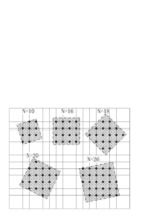
Figure 1: (Color online) Two-dimensional square structures for different system sizes N=10,16,18,20,26.

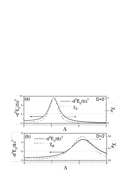
Figure 2: (Color online) The second derivative of ground-state energy (solid line) and fidelity susceptibility (dash line) of $N=20$ square lattice as a function of $\Delta$ for (a) $D=0$ and (b) $D=2$.

Next, to check whether these extreme points can be regarded as QCPs, we should perform FSS analysis, as is illustrated in Fig. 3. In Figs. 3(a) and 3(b), we plot FS per site as a function of $\Delta$ for different lattice size $N$=10, 16, 18, 20 and 26. As is clearly shown that $\chi_{\textrm{F}}$ becomes more pronounced for increasing $N$. $\chi_{\textrm{F}}$ is extensive in the off-critical region, while superextensive at the pseudocritical point. From the scaling relation Eq. (5), a linear dependence for the maximum fidelity susceptibilities $\chi_{\textrm{F}}^{\textrm{max}}$ on $L^{2/\nu}$ is expected with effective length $L=\sqrt{N}$. This is confirmed by the results shown in Figs. 3(c) and 3(d), in which we plot the logarithm of maximum fidelity susceptibilities $\chi_{\textrm{F}}^{\textrm{max}}$ at pseudocritical points verse a function of $\ln N$. For large $N$, $\ln\chi_{\textrm{F}}^{\textrm{max}}$ scales linearly with $\ln N$, and the slope is interpreted as the inverse of critical exponent of the correlation length $1/\nu$ from Eq. (5). By applying linear regression to the raw data obtained from XXZ model on various square lattices, we derive $1/\nu\approx 2.68(6)$ for $D=0$, while $1/\nu\approx 2.62(8)$ for $D=2$. The values got from the measurements of $D=0$ and $D=2$ are consistent with each other up to two digits. The validation of Eq. (5) implies that the QPT in 2D XXZ with DMI manifests itself as a clear sign of a second-order QPT.

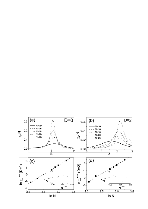
Figure 3: (Color online) Top: the fidelity susceptibility per site $\chi_{\textrm{F}}/N$ as a function of anisotropy parameter $\Delta$ for various size $N$= 10, 16, 18, 20, 26 with (a) $D=0$ and (b) $D=2$. Bottom: finite size scaling analysis for the height and location of the peaks. The logarithm of maximum fidelity susceptibilities $\chi_{\textrm{F}}^{\textrm{max}}$ for (c) $D$=0 and (d) $D$=2, respectively, are plotted as a function of $\ln N$. The dash lines are least square straight line fits with $1/\nu\approx 2.68(6)$ for (c) $D$=0 and $1/\nu\approx 2.62(8)$ for (d) $D$=2. The insets in panels (c) and (d) show pseudocritical points $\Delta_{L}^{*}$ for various sizes $N$ correspondingly.

From Figs. 3(a) and 3(b), the positions of cusps seemingly converge toward the critical points. However, these system sizes seem insufficiently to estimate the critical exponents from Eqs. (6) and (7), and the corrections to scaling relations are not negligible. In this case, the shift of the location of the pseudocritical point from real critical point should be replaced with $|\Delta_{L}^{*}-\Delta_{c}|\approx c_{1}L^{-1/\nu}+c_{2}L^{-2/\nu}+\ldots$, where $c_{1}$ and $c_{2}$ are the coefficients Zanardi-PRA-2008 . As is shown in insets of Figs. 3(c) and 3(d), we notice that the data points corresponding to the small system sizes clearly deviate from the linear fit obtained for the points for the two largest $N$. As $N\to\infty$, the pseudocritical points $\Delta_{L}^{*}$ approach the critical points $\Delta_{c}$. The linear fits from results of $N=20$ and $N=26$ (see Fig. 1) yield the estimates the $\Delta_{c}$ are $1.02$ and $2.47$, respectively. To get more precise critical exponents, more elaborate schemes are needed, such as large-scale quantum Monte Carlo simulations Schwandt-PRL-2009 ; Schwandt-PRB-2010 .

To proceed, we calculate the FS on $N$=20 square lattice for different sets of parameters $\Delta$ and $D$. The FS as a function of $D$ for $\Delta=1.5$ and $\Delta=2.0$ are depicted in Fig. 4, and the FS as a function of $\Delta$ for $D$=0, 1, 2, and 3 are plotted in Fig. 5. A boost of $\Delta$ and $D$ suppress the FS. By retrieving the critical points from the locations of FS peaks, we are able to draw the corresponding phase diagrams. The pseudocritical lines in the $(D,\Delta)$ plane and the $(\Delta,D)$ plane are shown in the insets of Fig. 4 and Fig. 5. We can notice that pseudocritical line for $N=20$ (solid dotted line) are qualitatively similar to the critical line in the thermodynamic limit (dash line).

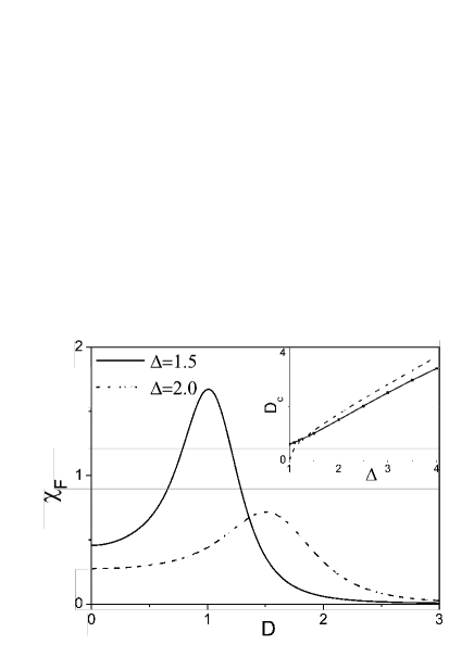
Figure 4: (Color online) The fidelity susceptibility $\chi_{\textrm{F}}$ as a function of $D$ for $\Delta=1.5$ and $\Delta=2.0$. Inset shows the pseudocritical line retrieved from the peaks of fidelity susceptibility for $N=20$ (solid dotted line) and the critical line $D_{c}=\sqrt{\Delta^{2}-1}$ in thermodynamic limit (dash line).

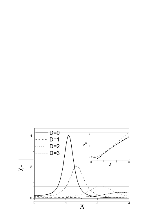
Figure 5: (Color online) The fidelity susceptibility $\chi_{\textrm{F}}$ in the ground state of the 2D 20-site XXZ model in terms of anisotropy for different values of DMI. Inset shows the pseudo critical line by the extraction from the maximum points of the fidelity susceptibility (solid dotted line), and the critical line $\Delta_{c}=\sqrt{1+D^{2}}$ in thermodynamic limit (dash line).

IV Fidelity susceptibility in the 2D Kitaev-Heisenberg model

Since Kitaev introduced a spin 1/2 quantum lattice model with Abelian and non-Abelian topological phases, finding a physical realization of Kitaev model has triggered a tremendous amount of interest PhysRevLett.105.027204 . It is proposed that in iridium oxides A₂IrO₃, the strong spin-orbit coupling may lead to the desired anisotropy of the spin interaction. The Ir⁴⁺ ions in iridium oxides A₂IrO₃ can be effectively illustrated as spin half on a honeycomb lattice, where three distinct types of NN bonds are referred to as $\gamma=$ ($0^{\circ}$, $120^{\circ}$, $240^{\circ}$) bonds. To describe the competition between direct exchange and superexchange mechanisms, a so-called Kitaev-Heisenberg model was dedicated, i.e.,

$${\cal H}_{\textrm{KH}}=\sum_{<{\mathbf{i}}{\mathbf{j}}>||\gamma}-2\alpha S_{\mathbf{i}}^{\gamma}S_{\mathbf{j}}^{\gamma}+(1-\alpha)\mathbf{S}_{\mathbf{i}}\cdot\mathbf{S}_{\mathbf{j}}.$$ (14)

The Hamiltonian (14) has been parameterized, which encompasses a few well-known models. For $\alpha=0$, it reduces to the Heisenberg model on a hexagonal lattice, while it becomes exactly solvable ferromagnetic Kitaev model at $\alpha=1$. Another solvable point corresponds to $\alpha=1/2$, where it is unitarily equivalent to ferromagnetic Heisenberg model. The ground state of Hamiltonian (14) evolves from 2D Néel AFM state ($\alpha=0$) to stripy antiferromagnetism ($\alpha=1/2$), and to spin liquid ($\alpha=1$) as $\alpha$ increases. We perform exact diagonalization (ED) on two geometries with $N$=16 and $N$=24 (see Fig. 6) to calculate the GS energy $E_{0}$ and fidelity susceptibility $\chi_{\textrm{F}}$.

Figure 6: (Color online) Two-dimensional structures for system sizes $N$=16 and 24, which can be placed on a hexagonal lattice with periodic boundary conditions.

Figure 7: (Color online) (a) The second derivative of energy density $e_{0}$ verse $\alpha$ for $N=16$ and $N=24$. (b) Fidelity susceptibility per site $\chi_{\textrm{F}}/N$ as a function of $\alpha$.

The second derivative of energy density $e_{0}\equiv-E_{0}/N$ and FS per site $\chi_{\textrm{F}}/N$ as a function of coupling strength $\alpha$ are obtained by Lanczos calculation. As is illustrated in Fig. 7, two anomalies emerge when $\alpha$ increases from $0$ to $1$, indicating the system undergoes two phase transitions. The characterization of QPTs by FS is compatible with the second derivative of energy density. We find that they play similar roles in identifying the QPTs Chen-PRA-2008 . However, the former demonstrates more pronounced peaks than the latter (notice the $y$-axis is of a logarithmic scale). QPT from Néel-ordered to stripe-ordered phase takes place at $\alpha\approx 0.4$, and this order-to-order phase transition seems insensitive to system size $N$ for these two configurations. On the other hand, the second order-to-disorder phase transition at $\alpha\approx 0.8$ appears to be sensitive to $N$. The numerical calculations point out that the QPT around $\alpha=0.4$ is first-order, while there is no consensus on the character of the QPT around $\alpha=0.8$ HCJiang ; Fabien . However, it is difficult to carry on ED on larger cluster for the hexagonal geometry and substantiate the scaling behavior of 2D Kitaev-Heisenberg model unless sophisticated techniques are used Schwandt-PRL-2009 ; Schwandt-PRB-2010 .

V Reduced Fidelity Susceptibility in The 2D Compass model

In recent years, the 2D AFM QCM has attracted considerable attention due to its interdisciplinary character. On one hand, it plays an important role in describing orbital interactions in TMOs. On the other hand, 2D QCM is equivalent to Xu-Moore model Xu2004 and toric code model in a transverse field Vidal2009 , which could possibly be used to generate protected qubits realized by Josephson-coupled $p\pm ip$ superconducting arrays PhysRevB.71.024505 .

QCM is defined on a $N=L\times L$ square lattice with PBC by the Hamiltonian

$${\cal H}_{\textrm{QCM}}=J_{x}\sum_{\langle\mathbf{i,j}\rangle||\mathbf{e_{x}}}S_{\mathbf{i}}^{x}S_{\mathbf{j}}^{x}+J_{z}\sum_{\langle\mathbf{i,j}\rangle||\mathbf{e_{z}}}S_{\mathbf{i}}^{z}S_{\mathbf{j}}^{z},$$ (15)

where $\mathbf{e_{x},e_{z}}$ are unit vectors along the $x$ and $z$ directions, and $J_{x}$ ($J_{z}$) is the coupling in the $x$ ($z$) direction. $S_{\mathbf{i}}^{\alpha}$ ($\alpha$=$x$, $y$, $z$) are the pseudospin operators of lattice site $\mathbf{i}$ obeying $[S_{\mathbf{i}}^{\alpha},S_{\mathbf{j}}^{\beta}]=i\epsilon_{\alpha\beta\gamma}S_{\mathbf{i}}^{\gamma}\delta_{\mathbf{i,j}}$. There exists a first-order phase transition at the self-dual point, i.e., $J_{x}=J_{z}$, and it is widely believed that the phase transition belongs to first-order PhysRevB.72.024448 ; PhysRevB.75.144401 ; PhysRevLett.102.077203 ; Vidal2009 .

In the case of $L$ being even, this model is equivalent to the ferromagnetic QCM by rotating the pseudospin operators at one sublattice by an angle $\pi$ about $\hat{S}^{y}$-axis. The Hamiltonian (15) enjoys such commutation relation with the parity operators $\hat{P}_{j}$ and $\hat{Q}_{i}$, which are defined as

$$\hat{P}_{j}=\prod_{i=1}^{L}\left(2\hat{S}^{z}_{i,j}\right)=\prod_{i=1}^{L}\hat{\sigma}^{z}_{i,j},\>\>\>\>\>\>\>\hat{Q}_{i}=\prod_{j=1}^{L}\left(2\hat{S}^{x}_{i,j}\right)=\prod_{j=1}^{L}\hat{\sigma}^{x}_{i,j},$$ (16)

where indices $i$ and $j$ are the $x$- and $z$-component of lattice site $\bf i$. However, column parity operator $\hat{P}_{j}$ does not commute but anticommutes with row parity operator $\hat{Q}_{i}$. In such circumstance, the Hilbert space can then be decomposed into subspace $V(\{p_{j}\})$, where $p_{j}$ is the eigenvalue of $\hat{P}_{j}$ and is specified in each subspace. Since $\hat{P}_{j}^{2}=1$, $p_{j}$ can be either 1 or -1. The lowest energy of the Hamiltonian in the subspace $V(\{p_{j}\})$ is nondegenerate. In Ref. Brzezicki-PRB-2010 , the authors unraveled the hidden dimer order therein. The symmetries in these systems induce large degeneracies in their energy spectra, and make their numerical simulation tricky. Recently, the ground state of ${\cal H}_{\textrm{QCM}}$ is proven to reside in the most homogeneous subspaces $V(\{p_{j}=1\})$ and $V(\{p_{j}=-1\})$, in other words, they are two-fold degenerate You-JPA-2010 .

At this stage, a single-site pseudospin-flipping interaction will change the parity of the chain, contrary to the flipping terms in $H$. For example, $\hat{S}_{\bf i}^{x}$ or $\hat{S}_{\bf i}^{y}$ acting on one chain along $x$ direction will change the parity of the chain. For two-point correlation functions between sites ${\bf i}$ and ${\bf j}$ separated by $n$ sites, it is not difficult to yield

$$e_{nz}^{x} = (-1)^{n}\left\langle\Psi_{0}(\Lambda)\left|\hat{S}_{\bf i}^{x}\hat{S}_{{\bf i}+n\hat{z}}^{x}\right|\Psi_{0}(\Lambda)\right\rangle=0.$$ (17)

Similarly, $e_{nz}^{y}$=0, $e_{nx}^{y}=0$, $e_{nx}^{z}=0$. The only correlation functions surviving are $\mathcal{C}_{nx}\equiv 4e_{nx}^{x}$ and $\mathcal{C}_{nz}\equiv 4e_{nz}^{z}$, as are shown in Fig. 8 and inset of Fig. 11. As $J_{x}$ increases, $\mathcal{C}_{z}$ decreases while $\mathcal{C}_{x}$ increases accordingly. They become equal at $J_{x}$= $J_{z}$.

With these properties of the ground state $|\Psi_{0}\rangle$ of the 2D QCM, a simple form for the two-site density matrix is obtained,

$$\rho(\mathbf{i},\mathbf{j})=\mathbf{Tr}^{\prime}(|\Psi_{0}\rangle\langle\Psi_{0}|)=\frac{1}{4}\sum_{\alpha,\alpha^{\prime}=0}^{3}\langle\sigma_{\mathbf{i}}^{\alpha}\sigma_{\mathbf{j}}^{\alpha^{\prime}}\rangle\sigma_{\mathbf{i}}^{\alpha}\sigma_{\mathbf{j}}^{\alpha^{\prime}},$$ (18)

in which the prime means tracing over all the other pseudospin degrees of freedom except the two sites $\mathbf{i}$ and $\mathbf{j}$. $\sigma^{\alpha}$ are Pauli matrices $\sigma^{x}$, $\sigma^{y}$ and $\sigma^{z}$ for $\alpha$ = 1 to 3, and 2 by 2 unit matrix for $\alpha$=0. If the two pseudospins are linked by an $x$-type bond, we have

$$\rho_{x}(\mathbf{i},\mathbf{j})=\mathbf{Tr}^{\prime}(|\Psi_{0}\rangle\langle\Psi_{0}|)=4\langle S_{\mathbf{i}}^{x}S_{\mathbf{j}}^{x}\rangle S_{\mathbf{i}}^{x}S_{\mathbf{j}}^{x}+\frac{1}{4}I_{\mathbf{i}}I_{\mathbf{j}},$$ (19)

in which $I_{\mathbf{i}}$ and $I_{\mathbf{j}}$ are the 2 by 2 unit matrices. If translational invariance is preserved in the ground state $|\Psi_{0}\rangle$, the reduced density matrix can be simplified as

$$\rho_{x}(\mathbf{i},\mathbf{j})=-\mathcal{C}_{x}S_{\mathbf{i}}^{x}S_{\mathbf{j}}^{x}+\frac{1}{4}I_{\mathbf{i}}I_{\mathbf{j}}.$$ (20)

Similarly, if the two sites $\mathbf{i}$ and $\mathbf{j}$ are linked by $z$-type bond, we have

$$\rho_{z}(\mathbf{i},\mathbf{j})=-\mathcal{C}_{z}S_{\mathbf{i}}^{z}S_{\mathbf{j}}^{z}+\frac{1}{4}I_{\mathbf{i}}I_{\mathbf{j}}.$$ (21)

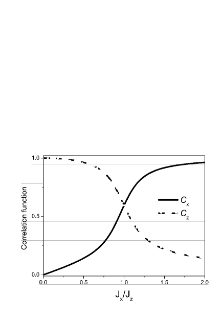
Figure 8: (Color online) The nearest-neighbor correlation functions $\mathcal{C}_{x}$ and $\mathcal{C}_{z}$ with respect to $J_{x}/J_{z}$ for $N=16$ square lattice. Two curves cross at $J_{x}/J_{z}$=1.

In addition, the NN two-point correlation functions $\mathcal{C}_{\alpha}$ can be calculated using the Feymann-Hellmann Theorem

$$\mathcal{C}_{\alpha}=-\frac{4}{N}\frac{\partial E_{0}}{\partial J_{\alpha}},$$ (22)

where $\alpha=x,z$ means $x$-type and $z$-type bond respectively.

The reduced fidelity $F_{\textrm{r}}$ is defined as the overlap between $\rho_{\alpha}(\mathbf{i},\mathbf{j})$ and $\rho^{\prime}_{\alpha}(\mathbf{i},\mathbf{j})$, i.e.

$$F_{\textrm{r}}(\rho_{\alpha}(\mathbf{i},\mathbf{j}),\rho^{\prime}_{\alpha}(\mathbf{i},\mathbf{j}))=\mathbf{Tr}\sqrt{\rho_{\alpha}^{1/2}\rho_{\alpha}^{\prime}\rho_{\alpha}^{1/2}}.$$ (23)

The prime means a different reduced density matrix induced by the tiny changes of driving parameters in the Hamiltonian. By Eqs. (20) and (21), it is obvious that $\rho_{\alpha}$ commutes with $\rho^{\prime}_{\alpha}$, and we can easily evaluate the reduced fidelity

$$F_{\textrm{r}}(\rho_{\alpha}(\mathbf{i},\mathbf{j}),\rho^{\prime}_{\alpha}(\mathbf{i},\mathbf{j})) = \frac{1}{2}\left(\sqrt{(1+\mathcal{C}_{\alpha})(1+\mathcal{C}^{\prime}_{\alpha})}\right.$$ (24)

$$+ \left.\sqrt{(1-\mathcal{C}_{\alpha})(1-\mathcal{C}^{\prime}_{\alpha})}\right).$$

The two-site RFS $\chi_{\textrm{r}}$ could also be obtained straightforwardly,

$$\chi_{\textrm{r}}^{\alpha\beta} = \lim_{\delta J_{\beta}\to 0}\frac{-2\ln F_{\textrm{r}}}{(\delta J_{\beta})^{2}}=\frac{(\partial_{J_{\beta}}\mathcal{C}_{\alpha})^{2}}{4(1-\mathcal{C}_{\alpha}^{2})},$$ (25)

in which $J_{\beta}$ ($\beta$=$x$,$z$) is the driving parameter for the QPT. According to Eqs. (22) and (25), we observe that the numerator of $\chi_{\textrm{r}}^{\alpha\alpha}$ is proportional to the square of the second derivative of GS energy and the denominator is finite in unpolarized state. The second power in the numerator indicates that the two-site RFS is more effective than the second derivative of the GS energy in measuring QPTs Xiong-PRB-2009 . We compare the RFS of two NN sites with the second derivative of GS energy of $N=18$ square lattice (see Fig. 1) displayed in Fig. 9, and find that they indeed present cusp-shaped peaks, but the former is more sensitive to phase transition than the latter. The pronounced maxima of peaks arise at $J_{x}/J_{z}=1$.

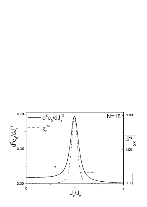
Figure 9: (Color online) The second derivative of ground state energy (solid line) and reduced fidelity susceptibility (dash line) of $N=18$ square lattice as a function of $J_{x}/J_{z}$.

Fig. 10 unveils the results from ED on various 2D square lattices with PBC. As the coupling $J_{x}$ changes, both FS and RFS of two NN sites exhibit peaks around $J_{x}=J_{z}$. With increasing system size, the peaks of $\chi_{\textrm{F}}$ (or $\chi_{\textrm{r}}$) become more pronounced and pseudocritical points seemingly converge toward the real critical point $J_{x}=J_{z}$ quickly. We plot the maximum fidelity $\chi_{\textrm{F}}^{\textrm{max}}$ and maximum reduced fidelity susceptibility $\chi_{\textrm{r}}^{\textrm{max}}$ against the system size $N$ in Fig. 10(d). The scaling of the peaks reveals approximately exponential divergences at criticality instead of power-law divergences, which indicates the occurrence of non-second-order phase transition.

As is argued in Eqs. (8) - (10), the approximately exponential divergence of FS and RFS hints an exponentially small gap at the critical point and thus a first-order phase transition. For two next-nearest-neighbor (NNN) sites, we calculate the RFS according to Eq. (25). We observe a similar behavior of the RFS with respect to $J_{x}/J_{z}$, and find that the RFS of NNN pair is a bit larger than the RFS of NN bond. This is illustrated in Fig. 11. In a word, the two-site RFS can serve as a signature for the QPTs in the 2D compass model.

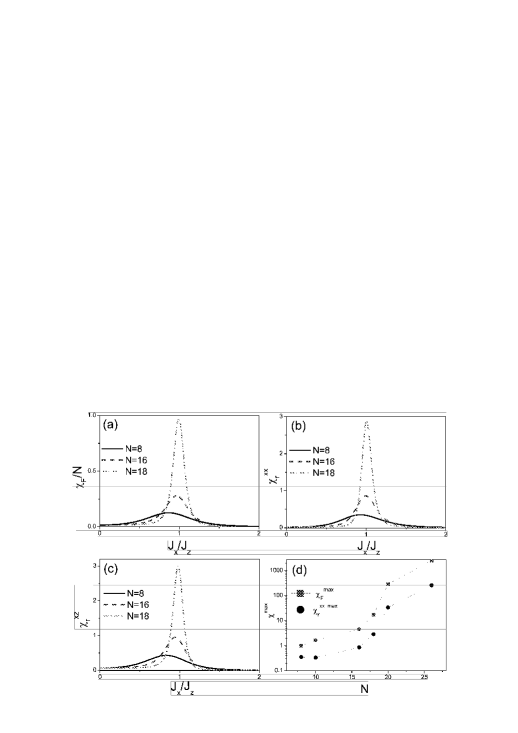
Figure 10: (Color online) (a) The fidelity susceptibility and (b) the reduced fidelity susceptibility of $x$-bond and (c) $z$-bond in the ground state of the 2D compass model on a square lattice as a function of $J_{x}/J_{z}$. The curves correspond to different lattice sizes $N$=8, 16 and 18, respectively. (d) The log-linear plot of maximum fidelity susceptibility and maximum reduced fidelity susceptibility against the system size $N$.

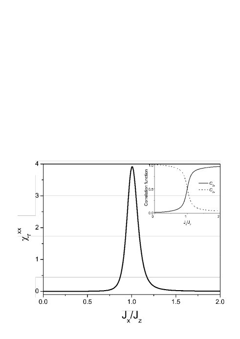
Figure 11: (Color online) The reduced fidelity susceptibility of two next-nearest-neighbor sites for $N=18$ square lattice with respect to $J_{x}/J_{z}$. Inset shows the next-nearest-neighbor correlation functions verse $J_{x}/J_{z}$.

VI Summary and Discussion

Motivated by recent theoretical and experimental work on orbital degree of freedom in Mott insulators, we have studied the QPTs in various 2D spin-orbit models using FS and RFS. The numerical analysis is performed on 2D clusters with the Lanczos algorithm. The spin-orbit model hosts plentiful phases, including phase transitions within and beyond the framework of Landau-Ginzburg paradigm. For the 2D XXZ model with DMI, with increasing driving parameters, the system undergoes a second-order phase transition from AFM state along $x$-$y$ plane to AFM state along $z$ direction. We compare FS with second derivative of GS energy, and find both of them exhibit similar peaks. The FSS demonstrates that FS per site should diverge in the thermodynamic limit at pseudocritical point, and the locations of extreme points approach QCPs accordingly. The power-law divergence of FS at criticality indicates the quantum phase transition is of second order and the critical exponent $\nu$ is obtained. Analogously, as the exchange coupling changes, the ground state of 2D Kitaev-Heisenberg model evolves from Néel AFM state to stripy AFM state, and to Kitaev spin liquid. The QCPs could be signaled by the peaks of both FS and second derivative of GS energy. The nonlocal symmetries in 2D AFM QCM guarantee that the RFS can be written in an analytical form as a function of the correlation functions. Peaks of FS and two-site RFS take place around $J_{x}$=$J_{z}$. The quasicritical point develops into critical point quickly with increasing the system size. Scaling of the peaks reveals an exponential divergence at criticality, which suggests that a first-order phase transition happens. In conclusion, the FS and RFS are effective tools in detecting diverse QPTs in 2D spin-orbit models, and their scaling behaviors may hint the orders of phase transitions.

VII ACKNOWLEDGMENTS

We acknowledge useful discussions with Wing-Chi Yu and J. Sirker. Wen-Long You acknowledges the support of the Natural Science Foundation of Jiangsu Province under Grant No. 10KJB140010 and the National Natural Science Foundation of China under Grant No. 11004144. Yu-Li Dong acknowledges the support of the Specialized Research Fund for the Doctoral Program of Higher Education (Grant No. 20103201120002), Special Funds of the National Natural Science Foundation of China (Grant No. 11047168) and the National Natural Science Foundation of China (Grant No. 11074184).

References

- (1) J. Zaanen, G. A. Sawatzky, and J.W. Allen, Phys. Rev. Lett. 55, 418 (1985).
- (2) Y. Tokura, and N. Nagaosa, Science. 288, 462 (2000).
- (3) S. W. Cheong, Nature Mater. 6, 927 (2007).
- (4) Anup Mishra, Michael Ma, Fu-Chun Zhang, Siegfried Guertler, Lei-Han Tang and Shaolong Wan, Phys. Rev. Lett. 93, 207201(2004).
- (5) K. I. Kugel and D. I. Khomskii, Sov. Phys. -JETP 37, 725 (1973).
- (6) Z. Nussinov and E. Fradkin, Phys. Rev. B 71, 195120 (2005).
- (7) J. Dorier, F. Becca, and F. Mila, Phys. Rev. B 72, 024448 (2005).
- (8) H.-D. Chen, C. Fang, J.-P. Hu, and H. Yao, Phys. Rev. B 75, 144401 (2007).
- (9) Román Orús, Andrew C. Doherty and Guifré Vidal, Phys. Rev. Lett. 102, 077203 (2009).
- (10) Sandro Wenzel and Wolfhard Janke, Phys. Rev. B 78, 064402 (2008).
- (11) Wojciech Brzezicki, Andrzej M. Oleś, Phys. Rev. B 80, 014405 (2009).
- (12) Ke-Wei Sun, Yu-Yu Zhang and Qing-Hu Chen, Phys. Rev. B 79, 104429 (2009).
- (13) W. Brzezicki, J. Dziarmaga, and A. M. Oleś, Phys. Rev. B 75, 134415 (2007).
- (14) Wen-Long You and Guang-Shan Tian, Phys. Rev. B 78, 184406 (2008).
- (15) B. Douçot, M. V. Feigel’man, L. B. Ioffe, and A. S. Ioselevich, Phys. Rev. B 71, 024505 (2005).
- (16) P. Milman, W. Maineult, S. Guibal, L. Guidoni, B. Douot, L. Ioffe, and T. Coudreau, Phys. Rev. Lett. 99, 020503 (2007).
- (17) G. Jackeli and G. Khaliullin, Phys. Rev. Lett. 102, 017205 (2009).
- (18) Wen-Long You, Guang-Shan Tian and Hai-Qing Lin, Phys. Rev. B 75, 195118 (2007).
- (19) Congjun Wu, Phys. Rev. Lett. 100, 200406 (2008).
- (20) A. Kitaev, Ann. Phys. (N.Y.) 321, 2 (2006).
- (21) S. Sachdev, Quantum Phase Transitions, (Cambridge University Press, Cambridge, UK, 2000)
- (22) Xiao-Yong Feng, Guang-Ming Zhang, and Tao Xiang, Phys. Rev. Lett. 98, 087204 (2007).
- (23) H. T. Quan, Z. Song, X. F. Liu, P. Zanardi, and C. P. Sun, Phys. Rev. Lett. 96, 140604 (2006).
- (24) P. Zanardi and N. Paunkovic, Phys. Rev. E 74, 031123 (2006).
- (25) Shi-Jian Gu, Int. J. Mod. Phys. B 24, 4371 (2010).
- (26) Wen-Long You, Ying-Wai Li and Shi-Jian Gu, Phys. Rev. E 76, 022101 (2007).
- (27) N. Paunkovic, P. D. Sacramento, P. Nogueira, V. R. Vieira, V. K. Dugaev, Phys. Rev. A 77 052302 (2008).
- (28) J. Ma, L. Xu, H. N. Xiong and X. Wang, Phys. Rev. E 78, 051126 (2008).
- (29) H. M. Kwok, C. S. Ho, S. J. Gu, Phys. Rev. A 78, 062302 (2008).
- (30) Wen-Long You and Wen-Long Lu, Phys. Lett. A 373, 1444 (2009) .
- (31) Zhi Wang, Tianxing Ma, Shi-Jian Gu, and Hai-Qing Lin,Phys. Rev. A 81, 062350 (2010).
- (32) Erik Eriksson and Henrik Johannesson, Phys. Rev. A 79, 060301(R)(2009).
- (33) H. M. Kwok, W. Q. Ning, S. J. Gu and H. Q. Lin, Phys. Rev. E 78, 032103 (2008).
- (34) Wing-Chi Yu, Ho-Man Kwok, Junpeng Cao, and Shi-Jian Gu, Phys. Rev. E 80, 021108 (2009).
- (35) S. J. Gu, H. M. Kwok, W. Q. Ning and H. Q. Lin, Phys. Rev. B 77, 245109 (2008).
- (36) M. A. Continentino, Quantum Scaling in Many-Body Systems (World Scientific Publishing, Singapore, 2001).
- (37) David Schwandt, Fabien Alet, and Sylvain Capponi, Phys. Rev. Lett. 103, 170501 (2009).
- (38) C. De Grandi, V. Gritsev, and A. Polkovnikov, Phys. Rev. B 81, 012303 (2010); Phys. Rev. B 81, 224301 (2010).
- (39) Marek M. Rams, Bogdan Damski, arXiv:1104.4104 (unpublished).
- (40) Silvano Garnerone, N. T. Jacobson, Stephan Haas, and Paolo Zanardi, Phys. Rev. Lett. 102, 057205 (2009).
- (41) N. T. Jacobson, Silvano Garnerone, Stephan Haas, and Paolo Zanardi, Phys. Rev. B 79, 184427 (2009).
- (42) L. Campos Venuti and P. Zanardi, Phys. Rev. Lett. 99, 095701 (2007).
- (43) Paolo Zanardi, Matteo G. A. Paris, and Lorenzo CamposVenuti, Phys. Rev. A 78, 042105 (2008).
- (44) Albuquerque, A. Fabricio and Alet, Fabien and Sire, Clément and Capponi, Sylvain, Phys. Rev. B 81, 064418 (2010).
- (45) C. De Grandi, A. Polkovnikov, A. W. Sandvik, arXiv:1106.4078 (unpublished).
- (46) Michael Kolodrubetz, David Pekker, Bryan K. Clark, Krishnendu Sengupta, arXiv:1106.4031 (unpublished).
- (47) Kurt Binder, Rep. Prog. Phys. 50, 783 (1987).
- (48) R. Schützhold, J. Low temp. Phys. 153, 228 (2008).
- (49) T. Jörg, F. Krzakala, J.Kurchan, A.C. Maggs and J. Pujos, EPL, 89, 40004 (2010).
- (50) O. F. Schirmer, A. Forster, H. Hesse, M. Wohleeke and S. Kapphan, J. Phys. C: Solid. State Phys. 17, 1321 (1984).
- (51) G. Cao, J. Bolivar, S. McCall, J. E. Crow, and R. P. Guertin, Phys. Rev. B 57, R11039 (1998).
- (52) S. J. Moon, M. W. Kim, K. W. Kim, Y. S. Lee, J.-Y. Kim, J.-H. Park, B. J. Kim, S.-J. Oh, S. Nakatsuji, Y. Maeno, I. Nagai, S. I. Ikeda, G. Cao, and T. W. Noh, Phys. Rev. B 74, 113104 (2006).
- (53) B. J. Kim, Hosub Jin, S. J. Moon, J.-Y. Kim, B.-G. Park, C. S. Leem, Jaejun Yu, T. W. Noh, C. Kim, S.-J. Oh, J.-H. Park, V. Durairaj, G. Cao, and E. Rotenberg, Phys. Rev. Lett. 101, 076402 (2008).
- (54) I. Dzyaloshinsky, J. Phys. Chem. Solids 4, 241 (1958).
- (55) T. Moriya, Phys. Rev 4, 288 (1960).
- (56) I. A. Sergienko and E. Dagotto, Phys. Rev. B 73, 094434 (2006).
- (57) Shuai Dong, Kunihiko Yamauchi, Seiji Yunoki, Rong Yu, Shuhua Liang, Adriana Moreo, J.-M. Liu, Silvia Picozzi, and Elbio Dagotto, Phys. Rev. Lett. 103, 127201 (2009).
- (58) Kh. Zakeri, Y. Zhang, J. Prokop, T.-H. Chuang, N. Sakr, W. X. Tang, and J. Kirschner, Phys. Rev. Lett. 104, 137203 (2010).
- (59) Thomas Michael and Steffen Trimper, Phys. Rev. B 82, 052401 (2010).
- (60) J. Honolka, T. Y. Lee, K. Kuhnke, A. Enders, R. Skomski, S. Bornemann, S. Mankovsky, J. Minár, J. Staunton, H. Ebert, M. Hessler, K. Fauth, G. Schütz, A. Buchsbaum, M. Schmid, P. Varga, and K. Kern, Phys. Rev. Lett. 102, 067207 (2009).
- (61) M. F. Yang, Phys. Rev. B 76, 180403(R) (2007).
- (62) Bo Wang, Mang Feng, and Ze-Qian Chen, Phys. Rev. A 81, 064301 (2010).
- (63) S. Chen, L.Wang, Y. Hao, and Y. Wang, Phys. Rev. A 77, 032111 (2008).
- (64) G. S. Tian and H. Q. Lin, Phys. Rev. B 67, 245105 (2003).
- (65) T. Kennedy, E. H. Lieb and B. S. Shastry, Phys. Rev. Lett. 61, 2582 (1988).
- (66) J. H. H. Perk and H. W. Capel, Phys. Lett. A 58 115 (1976).
- (67) D. N. Aristov and S. V. Maleyev, Phys. Rev. B 62, 751(R) (2000).
- (68) F. C. Alcaraz and W. F. Wreszinski, J. Stat. Phys. 58, 45 (1990).
- (69) Jiří Chaloupka, George Jackeli, and Giniyat Khaliullin, Phys. Rev. Lett. 105, 027204 (2010).
- (70) Hong-Chen Jiang, Zheng-Cheng Gu, Xiao-Liang Qi, and Simon Trebst, Phys. Rev B, 83, 245104 (2011).
- (71) Fabien Trousselet, Giniyat Khaliullin and Peter Horsch, Phys. Rev B, 84, 054409 (2011).
- (72) C. Xu and J. E. Moore, Phys. Rev. Lett. 93, 047003 (2004).
- (73) Julien Vidal, Ronny Thomale, Kai Philip Schmidt, and Sébastien Dusuel, Phys. Rev. B 80, 081104(R) (2009).
- (74) Wojciech Brzezicki and Andrzej M. Oleś, Phys. Rev. B 82, 060401(R) 2010.
- (75) W.-L. You, G.-S. Tian, and H.-Q. Lin, J. Phys. A 43, 275001 (2010).
- (76) Heng-Na Xiong,Jian Ma, Zhe Sun, and Xiaoguang Wang, Phys. Rev. B 79, 174425 (2009).