Optimal Eviction Policies for Stochastic Address Traces

Abstract

The eviction problem for memory hierarchies is studied for the Hidden Markov Reference Model (HMRM) of the memory trace, showing how miss minimization can be naturally formulated in the optimal control setting. In addition to the traditional version assuming a buffer of fixed capacity, a relaxed version is also considered, in which buffer occupancy can vary and its average is constrained. Resorting to multiobjective optimization, viewing occupancy as a cost rather than as a constraint, the optimal eviction policy is obtained by composing solutions for the individual addressable items.

This approach is then specialized to the Least Recently Used Stack Model (LRUSM), a type of HMRM often considered for traces, which includes $V-1$ parameters, where $V$ is the size of the virtual space. A gain optimal policy for any target average occupancy is obtained which (i) is computable in time $O(V)$ from the model parameters, (ii) is optimal also for the fixed capacity case, and (iii) is characterized in terms of priorities, with the name of Least Profit Rate (LPR) policy. An $O(\log C)$ upper bound (being $C$ the buffer capacity) is derived for the ratio between the expected miss rate of LPR and that of OPT, the optimal off-line policy; the upper bound is tightened to $O(1)$, under reasonable constraints on the LRUSM parameters. Using the stack-distance framework, an algorithm is developed to compute the number of misses incurred by LPR on a given input trace, simultaneously for all buffer capacities, in time $O(\log V)$ per access.

Finally, some results are provided for miss minimization over a finite horizon and over an infinite horizon under bias optimality, a criterion more stringent than gain optimality.

Keywords: Eviction policies, Paging, Online problems, Algorithms and data structures, Markov chains, Optimal control, Multiobjective optimization.

1 Introduction to Eviction Policies for the Memory Hierarchy

The storage of most computer systems is organized as a hierarchy of levels (currently, half a dozen), for technological and economical reasons [27] as well as due to fundamental physical constraints [13]. Memory hierarchies have been investigated extensively, in terms of hardware organization [22, 44, 27], operating systems [46], compiler optimization [3, 56, 26], models of computation [45], and algorithm design [1]. A central issue is the decision of which data to keep in which level. It is customary to focus on two levels (see Fig. 1), respectively called here the buffer and the backing storage, the extension to multiple levels being generally straightforward. (We adopt the neutral names used in the seminal paper of Mattson et al. [37], since the concepts introduced have application at each level of the memory hierarchy: register allocation, CPU caching, memory paging, web caching, etc.) We assume that an engine generates a sequence of access requests $a_{1},a_{2}\ldots,a_{t},\ldots$ for items (equally sized blocks of data) stored in the hierarchy. A request is called a hit if the requested item is in the buffer and a miss otherwise. Upon a miss, the item must be brought into the buffer, a costly operation. If the buffer is full, the requested item will replace another item. We are interested in an eviction policy that selects the items to be replaced so as to minimize subsequent misses.

The MIN policy of Belady [7] and the OPT policy of Mattson, Gecsei, Sluts, and Traiger [37], minimize the number of misses in an off-line setting. Since, in practical situations, the address trace unfolds with the computation, eviction decisions must be made on-line. Dozens of on-line policies have been proposed and implemented in hardware or within operating systems. Somewhat schematically, we can say that implemented policies have evolved mostly experimentally, by benchmarking plausible proposals against relevant workloads [44]. Most of these policies are variants of the Least Recently Used (LRU) policy. Departure from pure LRU is motivated to a large extent by its high implementation cost. However, several authors have also explored variants of LRU that incur fewer misses, at least on some workloads [38].

Figure 1: Two-level memory hierarchy.

Theoretical investigations have focused mostly on two objectives: (a) to “explain” the practical success of LRU-like policies and (b) to explore the existence of better policies. One major question is how to model the input traces (i.e., the lists of requested memory references). An interesting perspective, proposed by Koutsoupias and Papadimitriou [31], is to model traces by a class of stochastic processes, all to be dealt with by the same policy. For a given stochastic model, two metrics help assess the quality of a policy: (i) the expected number of misses and (ii) its ratio with the expected number of misses incurred by OPT, called the competitive ratio. The competitive ratio of a policy with respect to a class of stochastic processes is defined in a worst-case sense, maximizing over the class.

Competitive analysis was proposed by Sleator and Tarjan [47] for the class of all possible traces (all stochastic processes), for which they showed that the competitive ratio of any on-line policy is at least the buffer capacity $C$, a value actually achieved by, e.g., LRU and FIFO. While theoretically interesting, this results shed little light on what is experimentally known. For example, if we restrict the possible traces to the ones which actually emerge in practical applications, the miss ratio between LRU and OPT is much smaller than $C$, being typically around 2 and seldom exceeding 4. Borodin et al. [15] restrict the class of possible traces to be consistent with an underlying “access graph” that models the program locality (nodes correspond to items and legal traces correspond to walks); a heuristic policy based on this model has been developed by Fiat and Rosen [21] and has been shown to perform better than LRU, relative to some benchmarks.

Albers et al. [2] propose a trace restriction based on Denning’s working set concept [17]: for a given function $f(n)$, the (average or maximum) number of distinct items referenced in $n$ consecutive steps is at most $f(n)$. LRU is proved to be optimal in both the average and maximum cases.

Koutsoupias and Papadimitriou [31] have considered the class $\Delta_{\epsilon}$ ($0<\epsilon\leq 1$) of stochastic processes such that, given any prefix of the trace, the probability to be accessed next is at most $\epsilon$ for any item. A combinatorially rich development establishes that LRU achieves minimum competitive ratio, for each value of $\epsilon$. A careful analysis of how the competitive ratio depends upon both $\epsilon$ and $C$ has been provided by Young [59]: in particular, the competitive ratio increases with $\epsilon$. Qualitatively speaking, buffering is more efficient exactly when the items in the buffer are more likely to be referenced than those outside the buffer. Hence, for traces where LRU (or any policy) exhibits good performance (that is, few misses), $\epsilon$ must be correspondingly high. Then, the $\Delta_{\epsilon}$ competitive ratio is also high, unlike what observed in practice. For a more quantitative appraisal of the issue, consider that, at any level of the memory hierarchy of real systems, the average miss ratio is typically below 1/4 (even well below 1% in main memory). Let then $C_{1/2}$ be the buffer capacity at which the miss rate would be 1/2. It is easy to see that it must be $\epsilon C_{1/2}\geq 1/2$. The actual buffer capacity $C$ is typically considerably larger than $C_{1/2}$, say $C\geq 4C_{1/2}$, by the rule of thumb that quadrupling the cache capacity halves the miss ratio [44]. Then, $\epsilon C\geq 2$. By the bounds of Young [59], the $\Delta_{\epsilon}$ competitive ratio of LRU is at least $C/2$, which is not much more informative than the value $C$ of [47].

To “explain” both the low miss rate and the low competitive ratio of LRU in practical cases, the approach of [31] requires some restriction to the class of stochastic processes, in order to capture temporal locality of the reference trace, while essentially assigning low the probability to those traces for which OPT vastly outperforms LRU. The model and results of Becchetti [6] can be viewed as an exploration of this direction.

Following what could be viewed as an extreme case of the approach outlined above, a number of studies have focused on specific stochastic processes (the class is a singleton), with the objective of developing (individually) optimal policies for such processes. In [23], the address trace $a_{1},a_{2},\ldots,a_{t},\ldots$ is taken to be a sequence of mutually independent random variables, a scenario known as the Independent Reference Model (IRM). While attractive for its simplicity, the IRM does not capture the cornerstone property that memory hierarchies relay upon: the temporal locality of references. To avoid this drawback, the LRU-Stack Model (LRUSM) of the trace [40, 50] has been widely considered in the literature [55, 19, 30] and is the focus of much attention in this paper. Here, the trace is statistically characterized by the probability $s(j)$ of accessing the $j$-th most recently referenced item. The values of $j$ for different accesses are assumed to be statistically independent. Throughout, we assume that the items being referenced belong to a finite virtual space of size $V$. If $s$ is monotonically decreasing, LRU is optimal [50] (for an infinite trace); in general, the optimal policy varies with $s$ and can differ from LRU, as shown by Woof, Fernandez and Lang[57, 58]. Smaragdakis, Kaplan, and Wilson[48, 49] introduced the EELRU policy as a heuristic inspired by the LRUSM. The model of Becchetti [6] mentioned above is similar to LRUSM, essentially dropping the assumption of independence, while restricting the form of the conditional distribution of accessing the $j$-th most recent item, given the value of the past trace. LRU is compared to OPT under this model.

A different generalization of the IRM model is the Markov Reference Model (MRM), already suggested by [37], where the address trace is a finite Markov chain. A wealth of results are obtained by Karlin, Phillips, and Raghavan [29] for MRM, including the Commute Algorithm, a remarkable policy computable from the transition probabilities of the chain in polynomial time, whose expected miss rate is within a constant factor of optimum. We underscore that MRM and LRUSM are substantially different models; in general, while the MRM trace is itself a Markov process with $V$ states, the LRUSM trace is a function of a Markov process with $V!$ states.

Paper outline

In this work, we further the study of the LRUSM, deriving new results and strengthening its understanding. Some methodological aspects of our investigation, however, can be of interest for a wider class of models of the reference trace, hence they will be presented in a more general context.

A first methodological aspect we explore is the possibility as well as the fruitfulness of casting miss minimization as a problem of optimal control theory (or, equivalently, as a Markov Decision Problem [33]). In Section 2, we show as this is possible whenever the trace is a hidden Markov process, a scenario which we call the Hidden Markov Reference Model (HMRM). The IRM, the MRM, and the LRUSM are all special cases of the HMRM. We refer to the classical optimal control theory framework as presented, for instance, in the textbook of Bertsekas [11]. In the dynamical system to be controlled, the state encodes the content of the buffer and some information on the past trace. The disturbance input models the uncertainty in the address trace, while the control input encodes the eviction decisions available to the memory manager. The cost per step is one if a miss is incurred and zero otherwise. We modify the standard assumption that the control is a function only of the state and allow it to depend on the disturbance as well: $u_{t}=\mu_{t}(x_{t},w_{t})$. This modification is necessary since eviction decisions are actually taken with full knowledge of the current access. The Bellman equation characterizing the optimal policies has to be modified accordingly. The technicalities of this adaptation are dealt with in the Appendix.

A second methodological aspect we explore is a generalization of the buffer management problem where rather than imposing the capacity as a fixed constraint, we let the number of buffer positions vary dynamically, under the control of the management policy. The average buffer occupancy becomes a second cost, in addition to the miss rate, and the tradeoff between the two costs is of interest. This problem could have practical applications. For example, in a time-shared environment, processes could be charged for their average use of main memory and hence be interested in utilizing more memory in phases where this can result in significant page-fault reduction and less memory in other phases. In addition, the study of the average occupancy problem sheds significant light even on the solution of the fixed capacity problem. In particular, for the LRUSM, an optimal policy for the case of a fixed buffer can be simply obtained from optimal policies for the average occupancy case. In Section 3, the average buffer occupancy problem is studied for the HMRM, exploiting techniques of multi-objective optimization and optimal control. A key advantage lies in the possibility of composing a global policy from policies tailored to the individual items in the virtual space. Furthermore, the approach naturally lends itself to the efficient management of a buffer shared among different processes. Throughout this section, the notion of optimality of the policies under consideration is that of gain optimality over an infinite horizon.

In Section 4, the framework and the results developed in the two previous sections are applied to the LRUSM. After reviewing the LRU stack model, a class of optimal policies is derived, for an arbitrary distribution $s$, for the average occupancy problem. It is then shown that this class of policies includes some that use a buffer of fixed capacity $C$. More specifically, it is shown that the minimum miss rate under a constraint on the average occupancy can be attained with fixed capacity. A buffer of capacity $C$ is optimally managed by a $\operatorname{K-L}$ policy [57, 58], which can be specified by two parameters, denoted as $K=K(C)$ and $L=L(C)$. $\operatorname{K-L}$ policies include, as special cases, LRU ($K=C$, $\forall L$) and Most Recently Used (MRU) ($K=1$, $L=V$). Our derivation of the optimal policy has a number of advantages. (i) The optimality is established for the more general setting of average occupancy. (ii) The policy is naturally described in terms of a system of priorities for the eviction of items. As a corollary of a result of [37], it follows that the policy does satisfy the inclusion property: if an item is in a given buffer, then it is also in all buffers of larger capacity. The inclusion property rules out the so-called Belady anomaly [8] and enables more efficient algorithms for its performance evaluation. (iii) By linking the eviction priorities to the (planar) convex hull of the Pareto optimal points of the average occupancy problem and by adapting Graham’s scan, an algorithm is derived for a linear time computation of the values $K(C)$ and $L(C)$ for all relevant values of $C$. (Previously known properties of the $\operatorname{K-L}$ policy lead to a straightforward cubic algorithm.) (iv) Finally, the priorities can be shown to correspond to a suitable notion of profit rate of an item, informally capturing the best achievable ratio between expected hits and the expected occupancy for that item, leading to the concept of Least Profit Rate (LPR) policy. The LPR policy can be defined for models different from the LRUSM for which, while not necessarily optimal, it may yield a good heuristic.

In Section 5, we show that the ratio $\chi$ between the expected miss rate of the optimal on-line policy, LPR, and that of OPT is $O(\log C)$. Moreover, for the class of stack access distributions $s$ for which the miss rate of LPR is lower bounded by some constant $\beta>1/C$, we have $\chi\leq 2\ln(2/\beta)\in O(1)$.

The ability to efficiently compute the number of misses for buffers of various capacities when adopting a given policy for benchmark traces is of key interest in the design of hardware as well as software solutions for memory management [12, 52, 54]. In Section 6, we develop an algorithm to compute the LPR misses for all buffer capacities in time $O(\log V)$ per access, providing a rather non trivial generalization of an analogous result for LRU [9, 4].

In the remainder of the paper, we explore alternate notions of optimality. In Section 7, we consider optimization over a finite interval, or horizon. Technically, the optimal control problem is considerably harder. As an indication, even if the system dynamics, its cost function, and the statistics of the disturbance are all time invariant, the optimal control policy is in general time-dependent. We show that, for any monotonically non increasing stack distribution $s$, LRU is an optimal policy for any finite horizon, whereas MRU is optimal if the stack distribution is non decreasing. While these results appear symmetrical and highly intuitive, their proofs are substantially different and all but straightforward. The standard approach based on the Bellman equation, which requires “guessing” the optimal cost as a function of the initial state, does not seem applicable, lacking a closed form for such function. We have circumvented this obstacle by establishing an inductive invariant on the relative values of the cost for select pairs of states. This approach may have applicability to other optimal-control problems. Some of the results are derived for a considerably more general version of the LRUSM, which does not assume the statistical independence of stack distances at different steps.

Finally, in Section 8, we take a preliminary look at bias optimality, a property stronger than gain optimality, but also considerably more difficult to deal with. As an indication of the obstacles to be faced, we prove that, in some simple cases of LRUSM, no bias-optimal policy satisfies the useful inclusion property. We also develop a closed-form solution for the simplest non-trivial case of buffer capacity, that is, $C=2$. The derivation as well as the results are not completely straightforward, suggesting that the solution for arbitrary buffer capacity may require considerable ingenuity.

We conclude the paper with a brief discussion of directions for further research.

The main notation introduced and used throughout this work is summarized in Table 1.

Symbol	Description
$\operatorname{OPT}$	The (off-line) optimal replacement policy
$\operatorname{LRU}$	The Least Recently Used replacement policy
$\operatorname{LPR}$	The Least Profit Rate replacement policy
$V$	Size of the high-latency memory
$C$	Size of the low-latency buffer
$a_{t}$	Address of the item accessed at time $t$
$\Lambda_{t},d_{t}$	The $\operatorname{LRU}$ stack at time $t$ and $\operatorname{LRU}$ stack depth of item accessed at time $t+1$ ($\Lambda_{t}(d_{t})=a_{t+1}$)
$s(j)$	Probability of accessing the $j$-th most recently referenced item
$S(j)$	Cumulative probability distribution of $s$: $S(j)=\sum_{i=1}^{j}s(i)$
$\chi$	Stochastic competitive ratio
$x_{t}$	State at time $t$ (dynamical systems)
$w_{t}$	Disturbance at time $t$ (dynamical systems)
$u_{t}=\mu_{t}(x_{t},w_{t})$	Control at time $t$ (dynamical systems)
$x_{t+1}=f(x_{t},u_{t},w_{t})$	State transition (dynamical systems)
$g(x_{t},w_{t})$	Cost (dynamical systems)
$J^{*}_{t}(x_{0})$	Optimal cost starting from state $x_{0}$ with a time horizon of $t$ steps (dynamical systems)

Table 1: Main notation used throughout the paper

2 Optimal Control Formulation of Eviction for the Hidden Markov Reference Model

In the typical problem of optimal control [11], one is given a dynamical system described by a state-transition equation of the form

$$x_{t+1}=f(x_{t},u_{t},w_{t})\operatorname{\enspace,}$$ (1)

where $x_{t}$ is the state at time $t$, while both $u_{t}$ and $w_{t}$ are inputs, with crucially different roles. Input $u_{t}$, called the control, can be chosen by whoever operates the system. In contrast input $w_{t}$, historically called the disturbance, is determined by the environment and modeled as a stochastic process. At each step $t$, a cost is incurred, given by some function $g(x_{t},u_{t},w_{t})$. The objective of optimal control is to find a control policy $u_{t}=\mu_{t}(x_{t})$ so as to minimize the total cost

$$\operatorname{\mathbb{E}}_{w}\left[\sum_{t\in I}g(x_{t},u_{t},w_{t})\right]\operatorname{\enspace,}$$ (2)

where $I$ is a time interval of interest. A key premise of most optimal control theory is the assumption of past-independent disturbances (PID): given the current state $x_{t}$, the current disturbance $w_{t}$ is statistically independent of past disturbances $\{w_{\tau}:~{}\tau<t\}$.

In this section, we define a dynamical system whose optimal control corresponds to the minimization of the number of misses when the reference trace can be expressed as a function $a_{t}=r(z_{t})$ of a Markov chain $z_{t}$ with a finite state space $Z$. We call this scenario the Hidden Markov Reference Model (HMRM). In the following we assume the system to be unichain, i.e., under any stationary policy the Markov chain associated with the system evolution has only a single recurrent class. This hypothesis guarantees that the average cost in infinite horizon does not depend on the initial state and that there is always a solution to the Bellman equation (e.g., a Markov chain with two non communicating classes is not unichain).

To cast eviction as a problem in optimal control, the state of our dynamical system will model both the Markov chain underlying the trace and the content of the buffer:

$$x_{t}\mathrel{\mathop{:}}=(z_{t},b_{t})\operatorname{\enspace,}$$ (3)

where $b_{t}\in\{0,1\}^{V}$ is a Boolean vector such that, for $j=1,\ldots,V$,

$$b_{t}(j)\mathrel{\mathop{:}}=\begin{cases}1&j\text{ is in the buffer},\\ 0&\text{otherwise}.\end{cases}$$ (4)

Toward formulating the transition function governing the evolution of $x_{t}$, let us first observe that any Markov chain can be written as

$$z_{t+1}=\phi(z_{t},w_{t})\operatorname{\enspace,}$$ (5)

where $w_{t}\in W$ is a sequence of equally distributed random variables, independent of each other and of the initial state $z_{0}$ [32]. Furthermore, $W$ is a finite set with $|W|\leq|Z|(|Z|-1)$. We take $w_{t}$ to be the “disturbance” in (1). We let the control input $u_{t}\in\{0,1,\ldots,V\}$ encode the eviction decisions with $0$ denoting no eviction (the only admissible control in case of a hit) and $j>0$ denoting the eviction of the item $j$ (an admissible control only when a miss occurs and the item $j$ is in the buffer, i.e., $b_{t}(j)=1$). We can then write:

$$b_{t+1}=\psi(b_{t},u_{t})\operatorname{\enspace,}$$ (6)

where the transition function $\psi$ is specified as

$$b_{t+1}(j)\mathrel{\mathop{:}}=\begin{cases}1&j=a_{t}=r(z_{t})\operatorname{\enspace,}\\ 0&j=u_{t}\operatorname{\enspace,}\\ b_{t}(j)&\text{otherwise}\operatorname{\enspace.}\end{cases}$$ (7)

Finally, we have:

$$x_{t+1}=(z_{t+1},b_{t+1})=(\phi(z_{t},w_{t}),\psi(b_{t},u_{t}))=f(x_{t},u_{t},w_{t})\operatorname{\enspace.}$$ (8)

The instantaneous cost function $g$ is simply

$$g(x_{t},w_{t})\mathrel{\mathop{:}}=\begin{cases}1&\text{if a miss occurred}\operatorname{\enspace,}\\ 0&\text{otherwise}\operatorname{\enspace.}\end{cases}$$ (9)

Finally, we assume that a policy can set the control $u_{t}$ with knowledge of both the state and the disturbance: $u_{t}=\mu_{t}(x_{t},w_{t})$. This requires adaptation of some results derived in the control theory literature typically assuming $u_{t}=\mu_{t}(x_{t})$.

Consider a policy $\pi=\left(\mu_{1},\mu_{2},\ldots,\mu_{\tau}\right)$ applied to our system during the time interval $\left[1,\tau\right]$, so that, for $t$ in this interval, we have

$$x_{t+1}=f\left(x_{t},\mu_{t}\left(x_{t},w_{t}\right),w_{t}\right)\operatorname{\enspace.}$$ (10)

We define the cost of $\pi$, starting from state $x_{0}$, with time horizon $\tau$ as

$$J_{\tau}^{\pi}\left(x_{0}\right)\mathrel{\mathop{:}}=\operatorname{\mathbb{E}}_{\mathchoice{\mbox{\boldmath$\displaystyle w$}}{\mbox{\boldmath$\textstyle w$}}{\mbox{\boldmath$\scriptstyle w$}}{\mbox{\boldmath$\scriptscriptstyle w$}}}\left[\sum_{t=0}^{\tau-1}g\left(x_{t},w_{t}\right)\right],\quad\text{where }\mathchoice{\mbox{\boldmath$\displaystyle w$}}{\mbox{\boldmath$\textstyle w$}}{\mbox{\boldmath$\scriptstyle w$}}{\mbox{\boldmath$\scriptscriptstyle w$}}=\left[w_{0},w_{1},\ldots,w_{\tau-1}\right]\operatorname{\enspace,}$$ (11)

where the $x_{t}$’s are subject to (10) and the expected value averages over disturbances $w_{t}$. For our system, this is the expected number of misses in $\tau$ steps. The optimal cost is

$$J^{*}_{\tau}(x_{0})\mathrel{\mathop{:}}=\min_{\pi}J_{\tau}^{\pi}\left(x_{0}\right)\operatorname{\enspace.}$$ (12)

The optimal cost satisfies the following dynamic-programming recurrence (analogous to Eq. 1.6 in Vol. 1 of [11])

$$\begin{split}J^{*}_{\tau}(x_{0})=\operatorname{\mathbb{E}}_{w}\left[\min_{u\in U(x_{0},w)}\left\{g(x_{0},w)+J^{*}_{\tau-1}\left(f\left(x_{0},u,w\right)\right)\right\}\right]\operatorname{\enspace,}\end{split}$$ (13)

where $U(x_{0},w)$ denotes the set of controls admissible when the state is $x_{0}$ and the disturbance is $w$. Introducing a vector $\mathchoice{\mbox{\boldmath$\displaystyle J$}}{\mbox{\boldmath$\textstyle J$}}{\mbox{\boldmath$\scriptstyle J$}}{\mbox{\boldmath$\scriptscriptstyle J$}}^{*}$ whose components are the values $J^{*}_{\tau}(x)$, in some chosen order of the states, (13) can be concisely rewritten as

$$\mathchoice{\mbox{\boldmath$\displaystyle J$}}{\mbox{\boldmath$\textstyle J$}}{\mbox{\boldmath$\scriptstyle J$}}{\mbox{\boldmath$\scriptscriptstyle J$}}^{*}_{\tau}=\operatorname{T}\mathchoice{\mbox{\boldmath$\displaystyle J$}}{\mbox{\boldmath$\textstyle J$}}{\mbox{\boldmath$\scriptstyle J$}}{\mbox{\boldmath$\scriptscriptstyle J$}}^{*}_{\tau-1}\operatorname{\enspace,}$$ (14)

where $\operatorname{T}$ is the (non-linear) optimal-cost update operator.

In applications where the temporal horizon of interest is long and perhaps not known a priori, one is interested in policies that are optimal over an infinite horizon; an added benefit is that such policies are provably stationary, under very mild conditions. Usually, the cost defined in (11) diverges as $\tau\rightarrow\infty$, thus alternate definitions of optimality are considered [11, 33, 5, 14], like gain and bias optimality.

Gain Optimality

refers to a policy $\mu^{*}$ that achieves the lowest average cost (that can be shown to be independent of $x$): $\mu^{*}=\arg\min_{\mu}\lim_{\tau\rightarrow\infty}{J^{\mu}_{\tau}(x)}/{\tau}$ .

Bias Optimality

refers to a policy $\mu^{*}$ that is as good as any other stationary policy for $\tau$ long enough, i.e., $\forall x\;\lim_{\tau\rightarrow\infty}J^{\mu}_{\tau}(x)-J^{\mu^{*}}_{\tau}(x)\geq 0$. (Note that a bias optimal policy is also gain optimal.)

In this work we mostly concentrate on the standard gain optimality concept (which corresponds to the miss rate minimization), but we also give some particular results for the stronger concept of bias optimality in Section 8. In Sections 3 and 8 we will use the classical Bellman equation, which characterizes optimal control policies in infinite horizon as solutions of a fixed point equation [11]. We show in A that the result holds in our model as well:

Proposition 1.

Let $\Delta$ be a dynamical system, with state space $X$, whose control $u_{t}$ can be chosen with knowledge of the disturbance $w_{t}$. If $\exists\lambda\,\exists\mathchoice{\mbox{\boldmath$\displaystyle h$}}{\mbox{\boldmath$\textstyle h$}}{\mbox{\boldmath$\scriptstyle h$}}{\mbox{\boldmath$\scriptscriptstyle h$}}:\quad\lambda\mathchoice{\mbox{\boldmath$\displaystyle 1$}}{\mbox{\boldmath$\textstyle 1$}}{\mbox{\boldmath$\scriptstyle 1$}}{\mbox{\boldmath$\scriptscriptstyle 1$}}+\mathchoice{\mbox{\boldmath$\displaystyle h$}}{\mbox{\boldmath$\textstyle h$}}{\mbox{\boldmath$\scriptstyle h$}}{\mbox{\boldmath$\scriptscriptstyle h$}}=\operatorname{T}\mathchoice{\mbox{\boldmath$\displaystyle h$}}{\mbox{\boldmath$\textstyle h$}}{\mbox{\boldmath$\scriptstyle h$}}{\mbox{\boldmath$\scriptscriptstyle h$}}$, then $\lambda$ is the optimal average cost of $\Delta$ and $\textstyle h$ is the vector of the differential costs of the states, i.e.

$$\forall x,y\in X\quad\lim_{\tau\rightarrow+\infty}J_{\tau}^{*}(x)-J_{\tau}^{*}(y)=h(x)-h(y)\operatorname{\enspace.}$$ (15)

In the rest of the paper devoted to infinite horizon, since the costs will be independent of the initial state $x_{0}$, we will simplify (and abuse a little) the notation by setting $J^{\mu}(x_{0})=J(\mu)$.

3 The Average Occupancy Eviction Problem

The classical form of the eviction problem, as reviewed in the Introduction, is based on the assumption of a fixed capacity buffer: when the buffer is full, an eviction is required every time a miss occurs, otherwise no eviction is performed. In this section, we consider a relaxed version of the eviction problem where the buffer is of potentially unlimited capacity ($C=V$ is actually sufficient) and a variable portion of it can be occupied at different times. The requirement that the item being referred must be kept in the buffer or brought in if not already there is retained. However, after an access (whether a hit or a miss), any item in the buffer, except for the one just accessed, can be evicted. In this relaxed buffer management scenario, in addition to the miss rate, an interesting cost metric is the average occupancy of the buffer. We call average occupancy eviction problem the minimization of the miss rate, given a target value for the average occupancy. This problem has direct applications, as mentioned in the Introduction. However, the study of average occupancy also sheds light on the fixed capacity version, as we will see in particular in the next section for the LRUSM. A key advantage of the average capacity problem is that its solution can be obtained by combining policies for the individual items considered in isolation.

3.1 The Single Item Problem

In this section we study eviction policies for single items from a multiobjective perspective [20, 39], i.e., we are not interested in optimizing a single objective, but in obtaining all the “good” policies.

When focusing on a single item, say $\omega$, a first simplification arises from the fact that the state of the buffer, denoted $\beta_{\omega}$, is just a binary variable, set to $1$ when the item is kept in the buffer and to $0$ otherwise. One also can restrict attention to the $\omega$-trace $a_{\omega,t}$, defined as $1$ when the item is referenced ($a_{t}=\omega$) and to $0$ otherwise. Clearly, if the full trace $a_{t}$ is a hidden Markov process, so is also the $\omega$-trace. However, in some cases, the $\omega$-trace can be described with fewer states, forming a set $Z_{\omega}$. For example, the reduction is dramatic for the LRUSM, where $|Z|=V!$ while $|Z_{\omega}|=V$, for every item $\omega$. In general, we can write

$$a_{\omega,t}=r_{\omega}(z_{\omega,t}),\quad\text{with }z_{\omega,t+1}=\phi_{\omega}(z_{\omega,t},w_{\omega,t})\operatorname{\enspace.}$$ (16)

Process $z_{\omega,t}$ is called the Characteristic Generator (CG) of item $\omega$. The control input $u_{\omega,t}\in\{0,1\}$ determines whether $\omega$ is evicted from the buffer ($u_{\omega,t}=1$), which is admissible only when the item is in the buffer at time $t$ ($\beta_{\omega,t}=1$) and it is not currently accessed ($a_{\omega,t}=0$). This amounts to specifying the function $\psi_{\omega}$ such that

$$\beta_{\omega,t+1}=\psi_{\omega}(\beta_{\omega,t},u_{\omega,t})\operatorname{\enspace.}$$ (17)

The overall state of the control system is then $x_{\omega}=(z_{\omega},\beta_{\omega})$, evolving as

$$x_{\omega,t+1}=f_{\omega}(x_{\omega,t},u_{\omega,t},w_{\omega,t})\operatorname{\enspace.}$$ (18)

We are interested into two types of cost: buffer occupancy and misses. Correspondingly, we introduce two instantaneous cost functions:

$$g_{\operatorname{oc},\omega}(x_{\omega,t},w_{\omega,t}) =\beta_{\omega,t} g_{\operatorname{ms},\omega}(x_{\omega,t},w_{\omega,t}) =\begin{cases}1,&\beta_{\omega,t}=0\;\wedge\;a_{\omega,t}=1\quad\text{(miss)}\\ 0,&\text{otherwise}\operatorname{\enspace.}\end{cases}$$ (19)

Obviously, there is a tradeoff between the two costs, occupancy being minimized by evicting the item as soon as possible and misses being minimized by never evicting it. The set of “good” solutions to multiobjective optimization problems is the Pareto set, i.e., the set of all policies whose costs are not dominated by the costs of other policies (Pareto points are also known as Efficient Points, EPs).

A peculiarity of multiobjective optimization problems is that, since we are studying tradeoffs among the costs, sometimes we can usefully introduce Randomized Mixtures of Policies (RMoPs) to obtain more points in the costs space. E.g., consider the problem of choosing a route every day from home to work between two possible routes $\mu_{1}$ and $\mu_{2}$, with costs $\mathchoice{\mbox{\boldmath$\displaystyle J$}}{\mbox{\boldmath$\textstyle J$}}{\mbox{\boldmath$\scriptstyle J$}}{\mbox{\boldmath$\scriptscriptstyle J$}}(\mu)$ defined by the driving time and gas used. If $\mathchoice{\mbox{\boldmath$\displaystyle J$}}{\mbox{\boldmath$\textstyle J$}}{\mbox{\boldmath$\scriptstyle J$}}{\mbox{\boldmath$\scriptscriptstyle J$}}(\mu_{1})=(20\text{ minutes},10\$)$ and $\mathchoice{\mbox{\boldmath$\displaystyle J$}}{\mbox{\boldmath$\textstyle J$}}{\mbox{\boldmath$\scriptstyle J$}}{\mbox{\boldmath$\scriptscriptstyle J$}}(\mu_{2})=(30\text{ minutes},5\$)$ by choosing every day with the same probability $\mu_{1}$ or $\mu_{2}$ we have long-run average costs equal to $(25\text{ minutes},7.50\$)$, which cannot be obtained by choosing always the same route. To properly define an RMoP for the average occupancy problem for a single item, we observe that there always exists a “hit” state $x^{*}=(z^{*},1)$ (with $r_{\omega}(z^{*})=1$) which is recurrent in the system evolution (otherwise the item frequency would be zero and there would not be need to buffer it). If we call $t_{1},t_{2},\ldots$ the times at which the system enters the recurrent state, then the problems of choosing an eviction policy in the intervals $[t_{i}+1,t_{i+1}]$ are independent; by randomly choosing for each interval between two policies we can obtain all the convex combinations of the costs of the original non-mixture policies (see Fig. 2). In more detail, if policies $\mu^{\prime}$ and $\mu^{\prime\prime}$ exist with $J_{\operatorname{oc}}(\mu^{\prime})=\eta^{\prime}$ and $J_{\operatorname{oc}}(\mu^{\prime\prime})=\eta^{\prime\prime}$ such that $C=\gamma\eta^{\prime}+(1-\gamma)\eta^{\prime\prime}$ for some $\gamma\in[0,1]$, we write $\mu=\operatorname{rand}_{\gamma}\left(\mu^{\prime},\mu^{\prime\prime}\right)$ to mean that $\mu$ is an RMoP that chooses $\mu^{\prime}$ with probability $\gamma$ and $\mu^{\prime\prime}$ with probability $1-\gamma$ (the random choice being made every time the system leaves the state $x^{*}$). Note that an analog equation holds also for the miss rate cost: $J_{\operatorname{ms}}(\mu)=\gamma J_{\operatorname{ms}}(\mu^{\prime})+(1-\gamma)J_{\operatorname{ms}}(\mu^{\prime\prime})$.

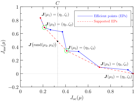
Figure 2: A Randomized Mixture of Policies (RMoP). Achieving $C$ as average buffer occupancy using a probabilistic combination of $\mu_{2}$ and $\mu_{3}$.

Since any point in the costs space between two policies can be obtained by an appropriate RMoP, the set of “good” policies in this context maps into the set $\cal{S}$ of Supported EPs (SEPs, also known as Pareto-convex points) which have costs not dominated by any convex combination of the costs of other policies. The set of SEPs can in general be of size exponential in $|Z_{\omega}|$ and thus it is interesting to find a polynomial approximation $\hat{\cal{S}}$ of $\cal{S}$. More specifically, for every point $(J_{1},J_{2})$ in $\cal{S}$ we want two points $({\hat{J}}_{1}^{\prime},{\hat{J}}_{2}^{\prime})$ and $({\hat{J}}_{1}^{\prime\prime},{\hat{J}}_{2}^{\prime\prime})$ in $\hat{\cal{S}}$ and a real number $0\leq\gamma\leq 1$ such that, for $q=1,2$, we have $J_{q}(1+\epsilon)\geq\gamma{\hat{J}}_{q}^{\prime}+(1-\gamma){\hat{J}}_{q}^{\prime\prime}$.

A necessary and sufficient condition [43, 18] to get a Polynomial Time Approximation Scheme (PTAS) to construct $\hat{\cal{S}}$ is the availability of a PTAS for solving the single-objective scalarized problem (Scal) which has the following cost:

$$G_{\omega,\theta}(x_{\omega},w_{\omega})=\cos(\theta)g_{\operatorname{oc},\omega}(x_{\omega},w_{\omega})+\sin(\theta)g_{\operatorname{ms},\omega}(x_{\omega},w_{\omega})\operatorname{\enspace.}$$ (20)

The PTAS to build $\hat{\cal{S}}$ runs in time polynomial in both $|Z_{\omega}|$ and $(1/\epsilon)$. (Note that any relative weight between the two costs can be achieved by a suitable choice of $\theta\in\left[0,\pi/2\right]$.) While Scal is interesting in its own right, here we are considering it mainly as a tool to find a polynomial approximation of the set of SEPs. For the single item problem the optimal policy solution of Scal can be obtained by solving the following Bellman equation [11], in the unknowns $\lambda_{\omega,\theta}\in\mathbb{R}$ and $h_{\omega,\theta}:X_{\omega}\rightarrow\mathbb{R}$, where $X_{\omega}=Z_{\omega}\times\{0,1\}$:

$$\lambda_{\omega,\theta}+h_{\omega,\theta}(x)=\operatorname{\mathbb{E}}_{w_{\omega}}\left[G_{\omega,\theta}(x_{\omega},w_{\omega})+\min_{u_{\omega}}\left\{h_{\omega,\theta}\left(f_{\omega}(x_{\omega},u_{\omega},w_{\omega})\right)\right\}\right]\operatorname{\enspace.}$$ (21)

The solution can be computed in time polynomial in $|Z_{\omega}|$ (the problem is P-complete [42]). The optimal policy can be obtained as $\mu_{\omega,\theta}(x_{\omega},w_{\omega})=\arg\min_{u_{\omega}}\left\{h_{\omega,\theta}\left(f_{\omega}(x_{\omega},u_{\omega},w_{\omega})\right)\right\}$. From the general theory, the cost of the optimal policy $\mu_{\omega,\theta}$ (for the instantaneous cost $G_{\omega,\theta}$) is $J_{\omega,\theta}=\lambda_{\omega,\theta}$. Standard methods permit the polynomial time computation of the values $J_{\operatorname{oc},\omega}$ and $J_{\operatorname{ms},\omega}$ of the same policy for the instantaneous costs $g_{\operatorname{oc},\omega}$ and $g_{\operatorname{ms},\omega}$, respectively.

3.2 The Average Occupancy of All Items

The solution for the average occupancy problem of all items can be obtained by choosing, for each item $\omega$, an appropriate solution (given in general by an RMoP) to the single item problem. In fact, let $\mu$ be an optimal policy for the all items problem, then $\mu$ induces an occupancy cost $J_{\operatorname{oc},\omega}(\mu)$ and a miss rate cost $J_{\operatorname{ms},\omega}(\mu)$ for each item $\omega$. Now consider the single item problem of finding a policy $\mu_{\omega}$ which minimizes $J_{\operatorname{ms},\omega}(\mu_{\omega})$ while achieving occupancy $J_{\operatorname{oc},\omega}(\mu_{\omega})=J_{\operatorname{oc},\omega}(\mu)$: then we must necessarily have $J_{\operatorname{ms},\omega}(\mu_{\omega})=J_{\operatorname{ms},\omega}(\mu)$, otherwise either $\mu$ or $\mu_{\omega}$ would be suboptimal. Because of this relationship between single and all items optimal policies, the average occupancy problem for all items reduces to a convex resource allocation problem, which can be solved efficiently [51, 53, 24], once we have the approximation of the set of SEPs for each single item.

A quantity of pivotal importance is the marginal gain $\rho_{\omega}$ of policy $\mu_{\omega}^{\prime}$ w.r.t. to policy $\mu_{\omega}$ defined, as

$$\rho_{\omega}\mathrel{\mathop{:}}=-\frac{J_{\operatorname{ms},\omega}(\mu_{\omega}^{\prime})-J_{\operatorname{ms},\omega}(\mu_{\omega})}{J_{\operatorname{oc},\omega}(\mu_{\omega}^{\prime})-J_{\operatorname{oc},\omega}(\mu_{\omega})}\operatorname{\enspace.}$$ (22)

The solution can be obtained in a greedy fashion by increasingly allocating buffer capacity to the item which provides a larger marginal gain. This greedy procedure takes time polynomial in $\sum_{\omega}|Z_{\omega}|$; a more sophisticated, asymptotically optimal algorithm can be found in [24]. Note that we can obtain the global miss rate $M$ and buffer occupancy $C$ just adding up the equivalent quantities for the single items:

$$M =\sum_{\omega}J_{\operatorname{ms},\omega}\operatorname{\enspace,} C =\sum_{\omega}J_{\operatorname{oc},\omega}\operatorname{\enspace.}$$ (23)

Theorem 1.

Let $\mathchoice{\mbox{\boldmath$\displaystyle J$}}{\mbox{\boldmath$\textstyle J$}}{\mbox{\boldmath$\scriptstyle J$}}{\mbox{\boldmath$\scriptscriptstyle J$}}(\mu^{1}_{\omega})=(\eta^{1}_{\omega},\zeta^{1}_{\omega}),\,\mathchoice{\mbox{\boldmath$\displaystyle J$}}{\mbox{\boldmath$\textstyle J$}}{\mbox{\boldmath$\scriptstyle J$}}{\mbox{\boldmath$\scriptscriptstyle J$}}(\mu^{2}_{\omega})=(\eta^{2}_{\omega},\zeta^{2}_{\omega}),\,\ldots$ be the list, with $\eta^{i}_{\omega}<\eta^{i+1}_{\omega}$, of the SEPs for the generic item $\omega$. The optimal policies $\mu_{\omega}$ (given for each item) are obtained applying Algorithm 1.

1$\forall\omega\;c[\omega]\leftarrow 1$ ;

2 $B\leftarrow 1$ ;

3 while $B<C$ do

4      

      // choose the policy improvement with maximum marginal gain

5       $\displaystyle\phi\leftarrow\arg\max_{\omega}\left\{-\frac{\zeta_{\omega}^{c[\omega]+1}-{\zeta_{\omega}^{c[\omega]}}}{\eta_{\omega}^{c[\omega]+1}-{\eta_{\omega}^{c[\omega]}}}\right\}$ ;

6       $B\leftarrow B+\eta_{\phi}^{c[\phi]+1}-{\eta_{\phi}^{c[\phi]}}$ ;

7       $c[\phi]\leftarrow c[\phi]+1$ ;

8      

9$\forall\omega\not=\phi\quad\mu_{\omega}\leftarrow\mu_{\omega}^{c[\omega]}$ ;

10 $\gamma\leftarrow\text{such that }B-\sum_{\omega\not=\phi}\eta_{\omega}^{c[\omega]}=\gamma\eta_{\phi}^{c[\phi]-1}+(1-\gamma)\eta_{\phi}^{c[\phi]}$ ;

11 $\mu_{\phi}\leftarrow\operatorname{rand}_{\gamma}\left(\mu_{\phi}^{c[\omega]-1},\mu_{\phi}^{c[\omega]}\right)$ ;

Algorithm 1 Obtaining the optimal algorithm for multiple items.

Remark 1.

Algorithm 1 will produce a non-mixture eviction policy for each item except for one, for which an RMoP may be needed in order to use the entire buffer space assigned to it. Note that, given a target value $C$ for the buffer occupancy, there exist a global policy made only of single item non-mixture policies which has average buffer occupancy $C-1<C^{\prime}\leq C$ and is optimal for that value of the occupancy.

3.3 Buffer Partitioning

An interesting application of the previous algorithm arises when we want to partition a buffer of capacity $C$ among $n$ independent processes, each described by a different HMRM. We assume that the $i$-th process accesses a private address space size $V_{i}$, at each step the $i$-th process has probability $\pi_{i}$ ($\sum_{i=1}^{n}\pi_{i}=1$) to be the one to run. We want to determine the capacity $C_{i}$ to devote to process $i$ (with $\sum_{i=1}^{n}C_{i}=C$) so as to minimize the global miss rate over an infinite temporal horizon, under the hypothesis that each process is using the optimal eviction policy.

It is straightforward to see that this problem is equivalent to building the global policy from single items with the cost $J_{\operatorname{ms}}$ of the items accessed by the $i$-th process rescaled by a factor $\pi_{i}$.

4 Optimal Policies for the LRUSM

In this section, we focus on stack optimal policies for the LRU Stack Model. After first reviewing the LRUSM (§4.1), we derive the optimal policy in the average occupancy framework (§4.2); due to the strong LRUSM structure many simplifications apply to the general procedure built in the previous section leading to a very efficient way of computing the optimal policy (linear in $V$). In §4.3 we focus on the fixed occupancy eviction problem and, by linking its solution to the average occupancy one, we are able to provide a stack eviction policy (Least Profit Rate, LPR) which is optimal for the LRUSM. Furthermore, we can fully characterize LPR behavior using a priority function based on a notion of profit which might be also of interest for other memory reference models.

4.1 The LRU Stack Model

Mattson et al. [37] observed that a number of eviction policies of interest, including LRU, MRU, and OPT, satisfy the following property.

Definition 1.

Given an eviction policy $\mu$ defined for all buffer capacities, let $B_{t}^{\mu}(C)$ be the content of the buffer of capacity $C$ at time $t$, after processing references $a_{1},\ldots,a_{t}$. We say that the inclusion property holds at time $t$ if, for any $C>1$, $B_{t}^{\mu}(C-1)\subseteq B_{t}^{\mu}(C)$, with equality holding whenever the bigger buffer is not full ($\left|B_{t}^{\mu}(C)\right|<C$). We say that $\mu$ is a stack policy if it satisfies the inclusion property at all times for all address traces, assuming that inclusion holds for the initial buffers $B_{0}^{\mu}(C)$, with $1\leq C\leq V$ (this is trivially verified if we assume, as we do, the initial buffers to be empty).

The optimal on-line policy LPR, developed in this section, is a stack policy. Inclusion protects from Belady’s anomaly [8] (i.e., increasing the buffer capacity cannot lead to a worse miss ratio, as can happen with, e.g., FIFO) and enables a compact representation of the content of the buffers of all capacities by the stack of the policy, an array $\Lambda^{\mu}_{t}$ whose first $C$ components yield the buffer of capacity $C$ as

$$B_{t}^{\mu}(C)=\left[\Lambda^{\mu}_{t}(1),\ldots,\Lambda^{\mu}_{t}(C)\right]\operatorname{\enspace.}$$ (24)

The stack depth $d_{t}$ of an access $a_{t+1}$ is defined as its position in the policy stack at time $t$, so that

$$a_{t+1}=\Lambda^{\mu}_{t}(d_{t})\operatorname{\enspace.}$$ (25)

Upon an access of depth $d$, a buffer incurs a miss if and only if $C<d$. Thus, computing the stack depth is an efficient way to simultaneously track the performance of all buffer capacities.

Figure 3: LRU stack update.

In the LRU stack, which we shall denote just by $\Lambda$ (i.e., $\Lambda=\Lambda^{\operatorname{LRU}}$), the items are ordered according to the time of their most recent access; in particular, $\Lambda_{t+1}(1)=a_{t+1}$. Upon an access at depth $d_{t}$, the LRU stack is updated by a downward, unit cyclic shift of its prefix of length $d_{t}$, as illustrated in Fig. 3. The LRU stack has inspired an attractive stochastic model for the address trace [40, 50, 55, 19, 30], where the access depths $d_{1},d_{2},\ldots$ are independent and identically distributed random variables, specified by the distribution

$$s(j)\mathrel{\mathop{:}}=\operatorname{Pr}[a_{t+1}=\Lambda_{t}(j)]=\Pr[d_{t}=j],\quad j=1,\ldots,V\enspace,$$ (26)

or, equivalently, by the cumulative sum

$$S(j)\mathrel{\mathop{:}}=\sum_{i=1}^{j}s(i),\quad j=1,\ldots,V\operatorname{\enspace.}$$ (27)

We assume that an “initial” LRU stack is given. W.l.o.g., $s(V)\not=0$ ($s(V)=0$ implies that the last page in the stack is never accessed and can therefore be ignored).

For example, the case where $s(j)$ decreases with $j$ captures a strict form of temporal locality, where the probability of accessing an item strictly decreases with the time elapsed from its most recent reference. It is simple to see that the actual trace $a_{1},a_{2},\ldots$ can be uniquely recovered from the stack-depth sequence $d_{1},d_{2},\ldots$, given the initial stack $\Lambda_{0}$.

To summarize, in the notation of Section 2, the state underlying the trace is the LRU stack ($z_{t}=\Lambda_{t}$) and the disturbance is the stack distance ($w_{t}=d_{t}$). We have a HMRM, since $a_{t+1}=r(\Lambda_{t+1})=\Lambda_{t+1}(1)$. The transition function $\phi$ for the trace state (such that $\Lambda_{t+1}=\phi(\Lambda_{t},d_{t})$) corresponds to the right unit cyclic shift of the the prefix of length $d_{t}$ of stack $\Lambda_{t}$. The control input $u_{t}$, the buffer state $b_{t}$, and the action of the former on the latter ($b_{t+1}=\phi(b_{t},u_{t})$) are according to the general definitions given in Section 2.

4.1.1 $\operatorname{K-L}$ Eviction Policies

A first optimal policy for the LRUSM was given by Wood, Fernandez and Lang in [57, 58]. They introduced the $\operatorname{K-L}$ eviction policy, defined as follows, in terms of LRU stack distance, for given integers $K$ and $L$ that $1\leq K<C\leq L\leq V$. If access $a_{t+1}$ results in a miss, then

• evict $\Lambda_{t+1}(L+1)$, if it is in buffer $B_{t}(C)$;

• otherwise evict $\Lambda_{t+1}(K+1)$, which is always in $B_{t}(C)$ if the policy is consistently applied starting from an empty buffer.

Here, $\Lambda$ denotes the LRU stack, while $B(C)$ denotes the content of the buffer under the $\operatorname{K-L}$ policy. Eviction is specified in terms of the LRU stack immediately after the rotation due to access $a_{t+1}$. Special cases are LRU ($K=C$, $\forall L$) and MRU ($K=1$, $L=V$). It has been shown in [57, 58] that, under the LRUSM, for any $C$, there exist values $K(C)$ and $L(C)$ for which the $\operatorname{K-L}$ policy is (gain) optimal. It is easily shown that, in the steady state, the items in the top $K$ positions of the LRU stack are always in the buffer, the items in the bottom $V-L$ positions are always outside the buffer, and $C-K$ of the $L-K$ items between position $K+1$ and $L$ are in the buffer. (Technically, the $\operatorname{K-L}$ policy is not specified for a buffer containing neither $\Lambda_{t+1}(L+1)$ nor $\Lambda_{t+1}(K+1)$. However, if the least recently used item is evicted in such case, one can show that the same steady state is reached, with probability 1.) It turns out that the miss rate of the $\operatorname{K-L}$ policy for a given distribution $s$ is

$$M^{\operatorname{K-L}}[s]=1-\frac{S(K)(L-C)+S(L)(C-K)}{L-K}\operatorname{\enspace.}$$ (28)

Finding, for each $C$, the optimal parameters $K(C)$ and $L(C)$ can be then accomplished in time $\Theta(V^{3})$, by evaluating the miss ratio for all possible $(K,L)$ pairs. In general, for a given $C$, the miss rate can be minimized by different $(K,L)$ pairs. Smaragdakis et al. [48, 49] proved that, for any given $s$, $K(C)$ and $L(C)$ can be chosen so that the resulting $\operatorname{K-L}$ policy does satisfy the inclusion property.

In the next subsection, we derive the optimal eviction policy in the average occupancy framework developed in Section 3 and highlight its deep structure. In §4.3 we derive a stack policy which is optimal in the fixed buffer model. By exploiting its similarity with the average occupancy optimal, we develop an algorithm that computes the two $K$ and $L$ parameters for all $C\in\{1,V\}$ in linear time, whereas a straightforward computation that does not exploit the stack policy characterization takes cubic time (a first speedup from cubic to quadratic is obtained exploiting the inclusion property, while the improvement from quadratic to linear derives from algorithmic refinements).

4.2 Average Occupancy Problem

The general procedure described in the previous section can be specialized for the LRUSM as follows. For each item $\omega$ the associated CG is a Markov chain $z_{\omega,t}$ with states $Z_{\omega}=\{1,\ldots,V\}$. The state encodes the position of the item in the LRU stack, thus satisfying the following transition probabilities:

$$\forall i\quad \operatorname{Pr}[z_{\omega,t+1}=1|z_{\omega,t}=i]=s(i)$$ (29)

$$\forall i\neq 1\quad \operatorname{Pr}[z_{\omega,t+1}=i|z_{\omega,t}=i]=S(i-1)$$ (30)

$$\forall i\neq V\quad \operatorname{Pr}[z_{\omega,t+1}=i+1|z_{\omega,t}=i]=1-S(i)\operatorname{\enspace.}$$ (31)

We also have $r_{\omega}(1)=1$ and, $\forall i\neq 1,\quad r_{\omega}(i)=0$. Thus, in the LRUSM the statistical description of the CGs is the same for all the items. The stationary eviction policies for the single item are binary vectors of size $V$ which say, for each LRU stack depth, if an item arriving at that position should be evicted. The “hit” state $x^{*}\mathrel{\mathop{:}}=(z^{*}=1,\beta=1)$, in which the item is at the top of the LRU stack and in the buffer, is recurrent and hence will be used to define RMoPs in the LRUSM: we assume an RMoP will choose a SEP policy each time the system leaves the state $x^{*}$. In the following we call lifetime the time between two consecutive $x^{*}$. A lifetime ends when the item is accessed. Thus, at the beginning of a new lifetime, an item is always at the top of the stack and in the buffer. If evicted from the buffer, the item will re-enter only at the beginning of the next lifetime.

We define $\operatorname{EV}_{k}$ as the policy which keeps the item in the buffer while at stack depth $i\leq k$ and evicts it if $i>k$. Note that, in steady state, any policy $\mu$ is equivalent to an appropriate $\operatorname{EV}_{k}$, where $k+1$ is the smallest depth at which the policy $\mu$ evicts (this is because, after the item is first accessed, it will always get evicted at depth $k+1$; it can only get evicted once at a different depth). Hence, w.l.o.g., we can limit our study to $\operatorname{EV}_{k}$ policies. To provide a close form for both the occupancy and the miss cost of $\operatorname{EV}_{k}$, we first need to establish some properties of the Markov chain $z_{\omega}$.

Proposition 2.

Let $t^{j}_{j+h}$ be the expected time spent by an item in position $j+h$ ($h\geq 0$) conditioned to the fact the item surely arrives in position $j$ without getting accessed. Then

$$t^{j}_{j+h}=\frac{1}{1-S(j-1)}\operatorname{\enspace.}$$ (32)

(Note that the expected time does not depend on $h$.)

Proof.

For $h=0$ we easily have that

$$t_{j}^{j}=1+S(j-1)t_{j}^{j}\quad\Rightarrow\quad t_{j}^{j}=\frac{1}{1-S(j-1)}\operatorname{\enspace.}$$ (33)

The event that an item starting from position $j$ does not arrive in position $j+1$ is the disjoint union of the events that there are exactly $h$ accesses with depth smaller than $j$ followed by one at depth $j$. So the probability for an item in position $j$ to arrive to position $j+1$ is

$$P_{j+1}^{j}=1-s(j)\sum_{h=0}^{+\infty}\left[S(j-1)\right]^{h}=\frac{1-S(j)}{1-S(j-1)}\operatorname{\enspace,}$$ (34)

and hence the expected time spent in position $j+1$ is

$$t_{j+1}^{j}=P_{j+1}^{j}t_{j+1}^{j+1}=\frac{1-S(j)}{1-S(j-1)}\frac{1}{1-S(j)}=t_{j}^{j}\operatorname{\enspace.}$$ (35)

Furthermore

$$t_{j+h}^{j}=P_{j+1}^{j}P_{j+2}^{j+1}\cdots P_{j+h}^{j+h-1}t_{j+h}^{j+h}=t_{j}^{j}\operatorname{\enspace.}$$ (36)

∎

As a special case, if we know that an item starts from position 1 (in which it is going to spend exactly one time step in the current lifetime) then it is going to spend an expected time $t_{j}^{1}=1$ in each position on the LRU stack in its lifetime and hence a lifetime has an expected length of $V$ timesteps. Under policy $\operatorname{EV}_{k}$, the item is buffered on average for $k$ timesteps per lifetime and hence the occupancy cost is given by

$$J_{\operatorname{oc}}(\operatorname{EV}_{k})=\frac{k}{V}\operatorname{\enspace.}$$ (37)

As for the miss rate, since the each position at depth $j>k$ contributes with a probability $s(j)$ to the misses, we have that

$$J_{\operatorname{ms}}(\operatorname{EV}_{k}) =\frac{1-S(k)}{V}\operatorname{\enspace.}$$ (38)

A direct application of Algorithm 1 would provide optimal policies $\mu_{\omega}$ identical for all the items except for on one (which, in general, will be managed by a RMoP). Actually, we can take a slightly different approach to exploit the CGs symmetry: by forcing the eviction policy to be the same for exactly all the items the global problem is reduced to the single-item one, with just a rescale of the costs $J_{\operatorname{oc}}$ and $J_{\operatorname{ms}}$ by a factor of $V$. The optimal policy is then an RMoP (the same for all the items) which mixes two eviction points corresponding to SEPs, causing each item to be evicted only at two possible stack depths. The next theorem summarizes the preceding discussion.

Theorem 2.

Let $q_{1}=1<q_{2}<\ldots<q_{l}=V$ be the values of $k$ such that $\operatorname{EV}_{k}$ is a SEP (i.e., a Pareto-convex) policy and let $q_{i}<C^{\prime}\leq q_{i+1}$, so that $C^{\prime}=\gamma^{\prime}q_{i}+(1-\gamma^{\prime})q_{i+1}$ for some $\gamma^{\prime}\in(0,1]$. Then, the RMoP that, for each item, mixes policies $\operatorname{EV}_{q_{i}}$ and $\operatorname{EV}_{q_{i+1}}$ with probability $\gamma^{\prime}$ and $(1-\gamma^{\prime})$, respectively, achieves optimal miss rate for average occupancy $C^{\prime}$.

It is a simple exercise to show that, if $s$ is monotonically decreasing, then $l=V$ and $q_{i}=i$. Instead, if $s$ is monotonically increasing, then $l=2$, $q_{1}=1$, and $q_{2}=V$.

4.3 Fixed Occupancy Problem

We have just shown that the optimal eviction policy in the average occupancy model is characterized by two eviction points in the LRU stack (let us call them $K^{\prime}(C)$ and $L^{\prime}(C)$). It is natural to investigate what happens by applying a $\operatorname{K-L}$ policy in the fixed occupancy model with $K=K^{\prime}(C)$ and $L=L^{\prime}(C)$. Under the $\operatorname{K-L}$ policy each lifetime is managed either by policy $\operatorname{EV}_{K}$ or $\operatorname{EV}_{L}$ and thus its occupancy $C$ and miss rate $M$ can be written as

$$C =\gamma J_{\operatorname{oc}}(\operatorname{EV}_{K})+(1-\gamma)J_{\operatorname{oc}}(\operatorname{EV}_{L}) M =\gamma J_{\operatorname{ms}}(\operatorname{EV}_{K})+(1-\gamma)J_{\operatorname{ms}}(\operatorname{EV}_{L})\operatorname{\enspace.}$$ (39)

A set of similar equations holds for the average occupancy setting:

$$C^{\prime} =\gamma^{\prime}J_{\operatorname{oc}}(\operatorname{EV}_{K^{\prime}})+(1-\gamma^{\prime})J_{\operatorname{oc}}(\operatorname{EV}_{L^{\prime}}) M^{\prime} =\gamma^{\prime}J_{\operatorname{ms}}(\operatorname{EV}_{K^{\prime}})+(1-\gamma^{\prime})J_{\operatorname{ms}}(\operatorname{EV}_{L^{\prime}})\operatorname{\enspace.}$$ (40)

Since $C=C^{\prime}$, $K=K^{\prime}$ and $L=L^{\prime}$ we must have the $\gamma^{\prime}=\gamma$. Then, we also have $M=M^{\prime}$, i.e., the miss rate achieved by the $\operatorname{K-L}$ policy for $K=K^{\prime}(C)$ and $L=L^{\prime}(C)$ is the same achieved by the average occupancy optimal. Since the optimal miss rate for average occupancy $C$ is obviously a lower bound for miss rate under fixed occupancy $C$, the choice $K=K^{\prime}(C)$ and $L=L^{\prime}(C)$ parameters yields an optimal policy under fixed capacity.

Based on these observations and on Theorem 2, we can compute, for each positive integer $C\leq V$, values $K(C)$ and $L(C)$ for a gain optimal, fixed capacity policy.

Corollary 1.

Given a stack-distance distribution $s$, the corresponding values $q_{1},q_{2},\ldots,q_{l}$ can be computed in time $\Theta(V)$ by Algorithm 2, a specialization of the Graham scan [25] to obtain the convex hall of planar sets of points. The same algorithm also computes optimal $K(C)$ and $L(C)$ for all (integer) buffer capacities $1\leq C\leq V$, uniquely determined from the $q_{i}$’s by the relation

$$K(C)=q_{i}<C\leq q_{i+1}=L(C)\operatorname{\enspace.}$$ (41)

Remark 2.

Because of costs (37) and (38) finding the SEPs is equivalent to find the convex hull of the set $\{(1,0)\}\cup\{(j,S(j))\}_{j}\cup\{(V,0)\}$. Since these points are already ordered along the first coordinate we can directly apply the linear phase of Graham scan, skipping the initial sorting. Finally, being the points equally spaced along the first coordinate, the algorithm reduces to finding, for each point $j$, the next point $i$ which maximizes the difference quotient:

$$\frac{S(i)-S(j)}{j-i+1}=\frac{\sum_{k=j}^{i}s(k)}{j-i+1}\operatorname{\enspace.}$$ (42)

This particular specialization of the Graham scan is studied in more detail in [10, 35].

// Graham scan specialization

1 $\nu[1]\leftarrow 1$;     $\pi[1]\leftarrow s(1)$;     $\Delta[1]\leftarrow 1$;

2 $\pi[V+1]\leftarrow 0$;     $\Delta[V+1]\leftarrow 1$;

3 for $j\leftarrow V$ downto $2$ do

4       $\nu[j]\leftarrow j$;     $\pi[j]\leftarrow s[j]$;

5       $\Delta[j]\leftarrow 1$;     $n\leftarrow\nu[j]+1$;

6       while $\pi[j]/\Delta[j]\leq\pi[n]/\Delta[n]$ do

7             $\nu[j]\leftarrow\nu[n]$;

8             $\pi[j]\leftarrow\pi[j]+\pi[n]$;

9             $\Delta[j]\leftarrow\Delta[j]+\Delta[n]$;

10             $n\leftarrow\nu[j]+1$;

11            

12      

// Print segmentation and priorities

13 $j\leftarrow 1$;     $i\leftarrow 1$;

14 while $j\leq V$ do

15       print “$q_{i}=\;$” , $\nu[j]$;

16       $j\leftarrow\nu[j]+1$;     $i\leftarrow i+1$;

17      

18$j\leftarrow 2$;

19 while $j\leq V$ do

20       print “$\xi(j)=\;$” , $\pi[j]/\Delta[j]$;

21       $j\leftarrow j+1$;

22      

Algorithm 2 Computing $K(C)$ and $L(C)$ and Profit Rates priorities – Linear algorithm. $K(C)=q_{i}<C\leq q_{i+1}=L(C)$ for some $i$.

4.3.1 The Least Profit Rate Eviction Policy

In this subsection we define a new stack policy, called Least Profit Rate ($\operatorname{LPR}$), by means of suitable priorities. We will see that, for any $C$, in steady state, the LPR policy becomes the same as the $K(C)$-$L(C)$ policy, and is therefore optimal.

Definition 2.

We define $\bar{s}(i,j)$ as the average of $s$ between $i$ and $j$:

$$\bar{s}(i,j)\mathrel{\mathop{:}}=\sum_{k=i}^{j}\frac{s(k)}{j-i+1}\operatorname{\enspace.}$$ (43)

Furthermore $\bar{s}(i)$ will indicate the moving average of $s$:

$$\bar{s}(i)\mathrel{\mathop{:}}=\bar{s}(1,i)\operatorname{\enspace.}$$ (44)

Definition 3.

Let $\omega$ be an item identified by its stack depth $i$ (i.e., $\Lambda(i)=\omega$). We define its profit rate $\xi$ as

$$\forall i\neq 1\quad\xi(i)\mathrel{\mathop{:}}=\max_{j}\bar{s}(i,j)\operatorname{\enspace.}$$ (45)

(The profit rate of the last accessed item $\Lambda(1)$ is not defined, since it cannot be evicted.)

Definition 4 (Least Profit Rate).

The $\operatorname{LPR}$ policy evicts the item $i^{*}$ in the buffer such that

$$i^{*}\mathrel{\mathop{:}}=\arg\min_{i}\xi(i)=\arg\min_{i}\max_{j}\bar{s}(i,j)\operatorname{\enspace.}$$ (46)

(If more items achieve the minimum, then the closest to the top of the stack is chosen.)

Next, we can state the main results of this section:

Theorem 3.

The $K(C)$-$L(C)$ eviction policies (for the various $C$) are uniquely determined by the LPR (whose definition does not depend on $C$).

Lemma 1.

Let $s$ be a function from natural to positive real numbers: $s:\mathbb{N}\rightarrow\mathbb{R}^{+}$. Let $\lambda$ be the point of maximum for $\bar{s}$. Then for each $q\leq\lambda$ we have

$$\bar{s}(\lambda)\leq\bar{s}(q,\lambda)\operatorname{\enspace.}$$ (47)

Proof.

We can rewrite $\bar{s}(\lambda)$ as

$$\bar{s}(\lambda)= \sum_{j=1}^{\lambda}\frac{s(j)}{\lambda}=\frac{q-1}{\lambda}\sum_{j=1}^{q-1}\frac{s(j)}{q-1}$$ (48)

$$+\frac{\lambda-q+1}{\lambda}\sum_{j=q}^{\lambda}\frac{s(j)}{\lambda-q+1}=$$ (49)

$$= \frac{q-1}{\lambda}\bar{s}(q)+\frac{\lambda-q+1}{\lambda}\bar{s}(q,\lambda)\operatorname{\enspace.}$$ (50)

Being $\bar{s}(\lambda)$ a convex combination of $\bar{s}(q)$ and $\bar{s}(q,\lambda)$ the following inequality holds:

$$\min\left\{\bar{s}(q),\bar{s}(q,\lambda)\right\}\leq\bar{s}(\lambda)\leq\max\left\{\bar{s}(q),\bar{s}(q,\lambda)\right\}\operatorname{\enspace.}$$ (51)

Since for hypothesis we have $\bar{s}(\lambda)\geq\bar{s}(q)$ we must have

$$\bar{s}(q)\leq\bar{s}(\lambda)\leq\bar{s}(q,\lambda)\operatorname{\enspace.}$$ (52)

∎

Lemma 2.

Let $s$ be a function from natural to positive real numbers: $s:\mathbb{N}\rightarrow\mathbb{R}^{+}$. Let $\lambda$ be the point of maximum for $\bar{s}$. Then for each $r>\lambda$ we have

$$\bar{s}(\lambda+1,r)\leq\bar{s}(\lambda)\operatorname{\enspace.}$$ (53)

Proof.

We have the following convex combination:

$$\bar{s}(r)=\frac{\lambda}{r}\bar{s}(\lambda)+\frac{r-\lambda}{r}\bar{s}(\lambda+1,r)\operatorname{\enspace,}$$ (54)

with $\bar{s}(\lambda)\geq\bar{s}(r)$ so we must have

$$\bar{s}(\lambda+1,r)\leq\bar{s}(r)\leq\bar{s}(\lambda)\operatorname{\enspace.}$$ (55)

∎

Remark 3.

Lemmas 1 and 2 highlight the following useful properties of the sequence $(q_{1},q_{2},\ldots,q_{l})$ obtained by Algorithm 2:

1. The average value of $s$ is strictly decreasing between segments: $\bar{s}(1+q_{i},q_{i+1})>\bar{s}(1+q_{i+1},q_{i+2})$

2. Within each segment the average of any prefix is smaller or equal to that of any suffix: $\forall k\in[1+q_{i},q_{i+1}]$, then $\bar{s}(1+q_{i},k)\leq\bar{s}(1+q_{i},q_{i+1})\leq\bar{s}(k,q_{i+1})$

Proof of Thm. 3.

Starting with an empty buffer we evict the first time when the top $C$ position of the LRU stack are filled. The position $i^{*}=\arg\min_{i}\max_{j}\bar{s}(i,j)$ is exactly $K+1$ (as can be seen applying Lemmas 1 and 2). The following position $l$ that has $\max_{j}\bar{s}(l,j)<\max_{j}\bar{s}(i^{*},j)$ is $L+1$, so each time an item reaches that position it is evicted (it can reach it only after a miss, since the positions after $L$ are not in the buffer). ∎

Below, we give a general formulation of the concepts of profit and of profit rate in the HMRM. For the definition we adopt the single item average occupancy model. Given an item $\omega$ and a time $t$, consider a single item eviction policy $\mu$ to determine, for any underlying state $z$ of the CG, whether $\omega$ is kept in the buffer or evicted upon reaching that state. We call $\mu$-profit of $\omega$ the probability $\pi^{\mu}$ that $\omega$ is referenced before it is evicted, which is a measure of how useful it would be to keep $\omega$ in the buffer under the policy. Let then $t+\Delta$, with $\Delta>0$, be the earliest time after $t$ such that $\omega$ is either referenced or evicted at time $t+\Delta$. Clearly, $\operatorname{\mathbb{E}}^{\mu}[\Delta]$ is a measure of the storage investment made on $\omega$ to reap that profit. Therefore, the quantity $\pi^{\mu}/\operatorname{\mathbb{E}}^{\mu}[\Delta]$ is a measure of profit per unit time, under policy $\mu$. Finally, we call profit rate of $\omega$ the maximum profit rate achievable for $\omega$, as a function of $\mu$. (It ought to be clear that profits and profit rates depend upon the current underlying state $z$ of the CG, although this dependence has not been reflected in the notation, for simplicity.)

As for the LRUSM, let consider a buffered item at position $i$ in the LRU stack. If we choose to keep it in the buffer until it goes past position $j$, then the item is going to spend on average the same time in each position between $i$ and $j$ and hence its profit per unit time will be $\bar{s}(i,j)$. This function has a maximum for some value of $j$ that defines the item profit rate, as shown above.

The Least Profit Rate (LPR) policy evicts, upon a miss, a page in the buffer with minimum profit rate. Profit rates are independent of buffer capacity, hence can be viewed as priorities. If ties are resolved consistently for all buffer capacities, LPR satisfies the inclusion property. In general, LPR is a reasonable heuristic, but not necessarily an optimal policy in the fixed occupancy model.

5 On-line vs. Off-line Optimality

Intuitively, the optimal off-line policy makes the best possible use of the complete knowledge of the future address trace, whereas the optimal on-line has only a statistical knowledge of the future. We compare these two information conditions via the stochastic competitive ratio, defined as the following functional of the distribution $s$:

$$\chi[s]\mathrel{\mathop{:}}=\frac{M^{\operatorname{LPR}}[s]}{M^{\operatorname{OPT}}[s]}\operatorname{\enspace,}$$ (56)

where $M^{\operatorname{LPR}}[s]$ and $M^{\operatorname{OPT}}[s]$ denote the expected miss rates (technically, the limit of the expected number of misses per step over an interval of diverging duration, as considered in gain optimality). The next theorem states the key result of this section.

Theorem 4.

For any stack access distribution $s$ and buffer capacity $C$, $\chi[s]=O(\ln C)$. If $M^{\operatorname{LPR}}[s]\geq\frac{1}{C}$, then the bound can be tightened as $\chi[s]\in O\left(\ln\frac{1}{M^{\operatorname{LPR}}[s]}\right)$.

To gain some perspective on the $O(\ln C)$ bound for LPR, we observe that the stochastic competitive ratio of LRU can be as high as $C$, (take $s:s(C+1)=1$). We also remark that, for classes of distributions where the miss rate of LPR is bounded from below by a constant, the competitive ratio is bounded from above by a corresponding constant.

Theorem  4 is established through several intermediate results:

1. A lower bound $L^{\operatorname{OPT}}[s]$ is developed for the (difficult to evaluate) quantity $M^{\operatorname{OPT}}[s]$, which yields a manageable upper bound to $\chi[s]$ (Prop. 3). (An analog lower bound for the deterministic case can be found in [41].)

2. An upper bound to the competitive ratio is evaluated for a quasi uniform distribution, which is analytically tractable (Prop. 4).

3. Finally, the analysis of the stochastic competitive ratio of an arbitrary distribution $s$ is reduced to that of a related, quasi uniform distribution $s^{\prime}$ (Prop. 5).

Steps 1 and 3 lead to the following chain of inequalities:

$$\chi[s]=\frac{M^{\operatorname{LPR}}[s]}{M^{\operatorname{OPT}}[s]}\leq\frac{M^{\operatorname{LPR}}[s]}{L^{\operatorname{OPT}}[s]}\leq\frac{M^{\operatorname{LPR}}[s^{\prime}]}{L^{\operatorname{OPT}}[s^{\prime}]}\operatorname{\enspace.}$$ (57)

Proposition 3.

Under the LRUSM, the miss rate of OPT is bounded from below as $M^{\operatorname{OPT}}[s]\geq L^{\operatorname{OPT}}[s]$, where, for $G\in\{1,\ldots,V-C\}$,

$$L^{\operatorname{OPT}}_{G}[s]\mathrel{\mathop{:}}=G\left(\sum_{j=0}^{C+G-1}\frac{1}{1-S(j)}\right)^{-1}\operatorname{\enspace,} L^{\operatorname{OPT}}[s]\mathrel{\mathop{:}}=\max_{G\in\{1,\ldots,V-C\}}L^{\operatorname{OPT}}_{G}[s]\operatorname{\enspace.}$$ (58)

Proof.

For a given value of $G$, we consider a partition of the trace $a_{1},a_{2},\ldots$ into consecutive segments, each minimal under the constraint that it contains exactly $C+G$ distinct references. Let $\tau_{i}$ denote the number of steps in the $i$-th such segment. The random variables $\tau_{1},\tau_{2},\ldots$ are statistically independent and identically distributed. Any one of them, generically denoted $\tau$, can be decomposed as

$$\tau\mathrel{\mathop{:}}=\sum_{j=0}^{C+G-1}\phi_{j}\operatorname{\enspace,}$$ (59)

where $\phi_{j}$ is the minimum number of steps, starting at some fixed time, to observe the first access with stack distance greater than $j$. It can be easily seen that $\phi_{j}$ is a geometric random variable, with parameter $p_{j}=1-S(j)$, $\operatorname{Pr}[\phi_{j}=k]=(1-p_{j})^{k-1}p_{j}$, expected value $1/p_{j}$, and finite variance. By linearity of expectation we have:

$$\operatorname{\mathbb{E}}[\tau]=\sum_{j=0}^{C+G-1}\frac{1}{1-S(j)}\operatorname{\enspace.}$$ (60)

Under any policy, including OPT, in each of the intervals of durations $\tau_{1},\tau_{2},\ldots$, there occur at least $G$ misses, since at most $C$ of the referenced items could be initially in the buffer. Therefore, we can write the following chain of relations:

$$\begin{split}M^{OPT}[s]\geq&\lim_{q\rightarrow\infty}\operatorname{\mathbb{E}}\left[\frac{qG}{\sum_{i=1}^{q}\tau_{i}}\right]=G\lim_{q\rightarrow\infty}\operatorname{\mathbb{E}}\left[\frac{1}{\bar{\tau}_{q}}\right]=G\operatorname{\mathbb{E}}\left[\frac{1}{\lim_{q\rightarrow\infty}\bar{\tau}_{q}}\right]=\frac{G}{\operatorname{\mathbb{E}}[\tau]}=L^{\operatorname{OPT}}_{G}[s]\operatorname{\enspace,}\end{split}$$ (61)

where $\bar{\tau}_{q}\mathrel{\mathop{:}}=\sum_{i=1}^{q}\frac{\tau_{i}}{q}$. The interchange between limit and expectation is justified because (i) by the law of large numbers, $\bar{\tau}_{q}$ converges in distribution to the delta peaked at $\operatorname{\mathbb{E}}[\tau]$ and (ii) the function $1/x$ is continuous and bounded within the support of $\bar{\tau}_{q}$ (which equals $\{x\in\mathbb{Z}:x\geq C+G\}$ since, for each $i$, $\tau_{i}\geq C+G$) [36]. ∎

Proposition 4.

Let $s^{\prime}$ be the distribution defined as

$$s^{\prime}(j)\mathrel{\mathop{:}}=\begin{cases}\sigma&j=1\\ \eta&j\in\{2,\ldots,V-1\}\\ \eta^{\prime}&j=V\end{cases}\operatorname{\enspace.}$$ (62)

Then the following lower bound for OPT miss rate holds:

$$M^{\operatorname{OPT}}[s^{\prime}]\geq L^{\operatorname{OPT}}[s^{\prime}]\geq\frac{V-C}{2}\left[1+\frac{1}{\eta}\ln\left(\frac{(V-2)\eta+\eta^{\prime}}{\left(\frac{V-2-C}{2}\right)\eta+\eta^{\prime}}\right)\right]^{-1}\operatorname{\enspace.}$$ (63)

Proof.

Applying Prop. 3 we can write

$$L^{\operatorname{OPT}}_{G}[s^{\prime}] =G\left[1+\sum_{j=1}^{C+G-1}\frac{1}{1-S(j)}\right]^{-1}=G\left[1+\sum_{j=1}^{C+G-1}\frac{1}{\eta^{\prime}+(V-j-1)\eta}\right]^{-1}$$ (64)

$$=G\left[1+\sum_{k=V-C-G}^{V-2}\frac{1}{\eta^{\prime}+k\eta}\right]^{-1}\geq G\left[1+\frac{1}{\eta}\ln\left(\frac{(V-2)\eta+\eta^{\prime}}{(V-C-G-1)\eta+\eta^{\prime}}\right)\right]^{-1}\operatorname{\enspace.}$$ (65)

By setting $G=\frac{V-C}{2}$ the thesis follows. ∎

Lemma 3.

If $\forall j\;S_{1}(j)\geq S_{2}(j)$ then $L^{\operatorname{OPT}}[s_{1}]\leq L^{\operatorname{OPT}}[s_{2}]$.

Proof.

From the definition of $L^{\operatorname{OPT}}$ we can see that it is decreasing with $\sum_{g=0}^{C+G-1}\frac{1}{1-S(g)}$, and hence decreasing with each $S(j)$. ∎

Proposition 5.

Let $s$ be an LRU stack access distribution, $C$ the buffer capacity and $\operatorname{LPR}$ its associated optimal online policy. Consider $s^{\prime}$ defined as follows:

$$s^{\prime}(j)=\begin{cases}\sigma&j=1\\ \eta&j\in\{2,\ldots,L+D\}\\ \eta^{\prime}&j=L+D+1\\ 0&j>L+D+1\end{cases}\operatorname{\enspace,}$$ (66)

where $\eta\mathrel{\mathop{:}}=\bar{s}(K+1,L)$, $\sigma\mathrel{\mathop{:}}=S(K)-(K-1)\eta$, $D\mathrel{\mathop{:}}=\left\lceil\frac{1-S(L)}{\eta}\right\rceil-1$, $\eta^{\prime}\mathrel{\mathop{:}}=1-S(L)-D\eta$ (note that $0<\eta^{\prime}\leq\eta$), then $s^{\prime}$ is a valid distribution and $L^{\operatorname{OPT}}[s^{\prime}]\leq L^{\operatorname{OPT}}[s]$ and $M^{\operatorname{LPR}}[s^{\prime}]=M^{\operatorname{LPR}}[s]$.

Proof.

We begin by observing (due to Lemmas 1 and 2) $\bar{s}(2,K)>\bar{s}(K+1,L)>\bar{s}(L+1,V)$. The transformation from $s$ to $s^{\prime}$ can be intuitively described as follows.

• We first “flatten” to $\eta=\bar{s}(K+1,L)$ the access distribution within the segment $[K+1,L]$ (in this operation no probability mass is moved outside the segment).

• We set $s(j)=\eta$ in the interval $[2,K]$. Since $\bar{s}(2,K)>\bar{s}(K+1,L)$ some probability mass is removed from $[2,K]$.

• We add to $s(1)$ the probability removed during the previous step.

• We redistribute the probability mass $1-S(L)$ at positions starting from $L+1$, assigning $\eta$ per position, possibly followed by a leftover $\eta^{\prime}$. This is possible because $\bar{s}(K+1,L)>\bar{s}(L+1,V)$.

After all these movements total probability mass is preserved and no position has a negative value, hence $s^{\prime}$ is still a valid distribution. Because of Lemmas 1 and 2 the transformation yields $\forall j\;S^{\prime}(j)\geq S(j)$ and hence, because of Lemma 3, $L^{\operatorname{OPT}}[s^{\prime}]\leq L^{\operatorname{OPT}}[s]$. As for LPR miss rate we have

$$M^{\operatorname{LPR}}[s]=1-S(L)+(L-C)\eta=(L+D-C)\eta+\eta^{\prime}=M^{\operatorname{LPR}}[s^{\prime}]\operatorname{\enspace.}$$ (67)

∎

Proof of Thm. 4.

Because of Prop. 5, given a distribution $s$ we can obtain a quasi uniform distribution $s^{\prime}$ (with a narrowed memory space $W\mathrel{\mathop{:}}=L+D+1\leq V$) such that

$$\chi[s]\leq\frac{M^{\operatorname{LPR}}[s^{\prime}]}{L^{\operatorname{OPT}}[s^{\prime}]}=\frac{\eta^{\prime}+(W-1-C)\eta}{W-C}\left[2+\frac{2}{\eta}\ln\left(\frac{(W-2)\eta+\eta^{\prime}}{\left(\frac{W-2-C}{2}\right)\eta+\eta^{\prime}}\right)\right]\mathrel{\mathop{:}}=\tilde{\chi}[s^{\prime}]\operatorname{\enspace.}$$ (68)

To simplify the analysis of $\chi[s]$ we can assume $C\gg 1$ and $W-C>2$ (the complementary case is easy to deal with). Equation (68) reduces to

$$\chi[s]\leq O(1)+2\ln\left(\frac{2(W-1)}{W-2-C}\right)\in O\left(\ln C\right)\operatorname{\enspace.}$$ (69)

Finally, since $M^{\operatorname{LPR}}[s]\leq(W-C)\eta$ and $\eta\leq\frac{1}{W-2}$ (since $s(1)+\eta^{\prime}+\eta(W-2)=1$) we have $M^{\operatorname{LPR}}[s]\leq\frac{W-C}{W-2}$, implying

$$\chi[s]\in O\left(\ln\frac{1}{M^{\operatorname{LPR}}[s]}\right)\operatorname{\enspace,}$$ (70)

which, for $M^{\operatorname{LPR}}[s]>\frac{1}{C}$, provides a more descriptive bound than (69). ∎

6 Fast Simulation of the LPR Policy

In experimental studies it is important to simulate eviction policies on sets of benchmark traces. From the stack distances, the number of misses for all buffer capacities can be easily derived in time $O(V)$. Previous work [9, 4] has shown how to compute the stack distance for the LRU policy in time $O(\log V)$ per access. We derive an analogous result for the more complex LPR policy.

Theorem 5.

Given any stack-distance distribution $s$, the number of misses incurred by the corresponding optimal LPR policy on an arbitrary trace of $N$ references, can be computed, simultaneously for all capacities, in time $O(V+N\log V)$.

The algorithm proposed to prove the preceding result exploits some relations between the LPR stack and the LRU stack and achieves efficiency by means of fast data structures.

Proposition 6.

Let $s$ be a stack-distance distribution and let $(q_{1},q_{2},\ldots,q_{l})$ be the (increasing) sequence associated with $s$ as in Theorem 2. Let $\Lambda$ be the LRU stack and let $\Pi$ be the LPR stack corresponding to $s$, both assumed initially equal. In either stack, let the $i$-th segment be the set of positions in interval $Q_{i}\mathrel{\mathop{:}}=[q_{i}+1,q_{i+1}]$. Finally, for $j\in\{1,2,\ldots,V\}$, let $\rho_{t}(j)$ denote the position in the LPR stack $\Pi_{t}$ of the item that is in position $j$ of the LRU stack $\Lambda_{t}$, i.e., $\Pi_{t}(\rho_{t}(j))$=$\Lambda_{t}(j)$. Then, we have:

1. Segment equivalence. At any time $t$, segment $Q_{i}$ contains the same items in both stacks, that is, $j\in Q_{i}$ if and only if $\rho_{t}(j)\in Q_{i}$.

2. Relative update. Upon an access $a_{t}$ at LRU stack depth $d_{t}$, if $d_{t}=1$, then the map $\rho$ between the two stacks is unchanged. Otherwise ($d_{t}>1$), $\rho$ is updated as follows. For any $t$, any segment $Q_{i}$, with $i=1,\ldots,l-1$, and any $h\in\{0,q_{i+1}-q_{i}-1\}$, (so that $(q_{i}+1+h)\in Q_{i}$), we have:

   $$\rho_{t+1}(q_{i}+1+h)=\begin{cases}\rho_{t}(q_{i}+1+h)&d_{t}<q_{i}+1+h\\ \rho_{t}\left(q_{i}+1+\left((h-1)\bmod(d_{t}-q_{i})\right)\right)&q_{i}+1+h\leq d_{t}\leq q_{i+1}\\ \rho_{t}\left(q_{i}+1+\left((h-1)\bmod(q_{i+1}-q_{i})\right)\right)&q_{i+1}<d_{t}\operatorname{\enspace.}\\ \end{cases}$$ (71)

   In other words, (a) below the LRU point of access, $\rho$ does not change; (b) within the prefix of the segment including the access up to the point of access itself, as well as (c) within those segments that are entirely above the point of access, $\rho$ incurs a unit, right cyclic shift.

Proof.

Segment equivalence. We begin by observing that, for buffer sizes in the set $\{q_{1},q_{2},\ldots,q_{l}\}$, the LPR policy coincides with LRU, whence $B_{t}^{LPR}(q_{i})=B_{t}^{LRU}(q_{i})$. In fact, for a $\operatorname{K-L}$ policy, the buffer content is a subset of the first $L$ positions of the LRU stack. From Corollary 1, if $C=q_{i}$, then $L(C)=q_{i}$, hence the LPR buffer content must equal that of the first $q_{i}$ positions of the LRU stack which, by definition of stack, is also the content of the LRU buffer of capacity $q_{i}$. The segment equivalence property follows since, for any stack policy, the content of the stack in a segment $Q_{i}$ equals (by definition) the set theoretic difference between $B(q_{i+1})$ and $B(q_{i})$.

Relative update. If $d_{t}=1$, then neither stack changes, therefore $\rho_{t+1}=\rho_{t}$. Otherwise, let $d_{t}\in Q_{a}$, that is, let $Q_{a}$ be the segment capturing the access and consider the following cases.

(i) For all buffer sizes $C>q_{a+1}$, the access is a hit both for the LRU and for the LPR policy, hence both stacks, and consequently the $\rho$ map, remain unchanged at positions greater than $q_{a+1}$. This is a subcase of case (a) in the statement and applies to all segments with $i>a$ (hence $1+q_{i}+h>q_{a+1}$).

(ii) For buffer sizes $C\in Q_{a}$ the situation is as follows. Under LRU, there is a miss for $C<d_{t}$, so that in the LRU stack: the items in positions smaller than $d_{t}$ shift down by one position, the item at $d_{t}$ goes at the top of the stack, and all other items retain their position. Under LPR, let $C_{a}$ be the smallest capacity of a buffer containing the referenced item, $a_{t+1}$. Then, all the buffers with $C<C_{a}$ will evict item $\Lambda_{t}(q_{a})$, which will go to position $C_{a}$ of the LPR stack, the item previously at $C_{a}$ will go to the top of the stack, while all remaining items in segment $Q_{a}$ will retain their position. Consequently, for $h=(d_{t}+1)-(q_{a}+1),\ldots,q_{a+1}-(q_{a}+1)$, we have $\rho_{t+1}(q_{a}+1+h)=\rho_{t}(q_{a}+1+h)$, still a subcase of case (a) in the statement. Furthermore, $\rho_{t+1}(q_{a}+1)=\rho_{t}(d_{t})$ and, for $h=1,\ldots,d_{t}-(q_{a}+1)$, $\rho_{t+1}(q_{a}+1+h)=\rho_{t}(q_{a}+1+h-1)$, which establishes case (b) in the statement.

(iii) For segments $Q_{i}$ with $i<a$, the argument is a straightforward adaptation of that developed for case (ii) and establishes case (c) of the statement.
∎

We are now ready to provide the algorithm for LPR stack-distance computation and its analysis.

Proof of Thm. 5.

The work of [9, 4] has provided a procedure that, given the initial LRU stack $\Lambda_{0}$ and the prefix $a_{1},\dots,a_{t}$ of the input trace, will output the LRU stack distances $d_{0},\ldots,d_{t-1}$, in time $O(V+t\log V)$. Below, we develop a representation of the map $\rho$ between the LRU and the LPR stack, which can be updated and queried in time $O(\log V)$ per access. Then the LPR stack distance of access $a_{t+1}$ can be obtained as $\rho(d_{t})$.

By Proposition 6, we can represent $\rho$ by a separate sequence $(\rho(q_{i}+1),\ldots,\rho(q_{i+1}))$ for each segment. On such a sequence, we need to perform cyclic shifts of an arbitrary prefix and to access element $\rho(q_{i}+1+h)$, given an $h\in[0,q_{i+1}-(q_{i}+1)]$. Any of the well-known dynamic balanced trees (AVL, 2-3, red-black, …) [16] can be easily adapted to perform each of the required operations in time $O(1+\log(q_{i+1}-q_{i}))=O(\log V)$. Hereafter, we denote by $R_{i}$ the data structure for segment $Q_{i}$.

The number of segments where the map $\rho$ can change in one step can be $\theta(V)$, in the worst case. Therefore, we adopt a lazy update strategy whereby only the segment $Q_{a}$ capturing the access is actually updated; for the other segments, record is taken that a shift should be applied to the sequence, without performing the shift itself. It is sufficient to increment a counter storing the amount of shift that has to be applied to the sequence and then perform just one global rotation when the segment is accessed. Still, individually incrementing each segment counter could lead to work proportional to $V$, per step. Instead, we maintain an auxiliary tree $T$ of counters which collectively serve the segments and where at most logarithmically many counters need updating in a given step. A further field in the auxiliary tree will enable quick identification of segment $Q_{a}$.

More specifically, the auxiliary tree is a static, balanced tree with $l-1$ leaves corresponding, from left to right, to segments $Q_{1},\ldots Q_{l-1}$. In each internal node, a search field contains the maximum right boundary of any segment associated with a descendant of that node. In each node, a counter field will be maintained so that, at the end of a step, the sum of the counters over the ancestors of the $i$-th leaf represent the amount of shift to be applied to $\rho$-sequence in segment $Q_{i}$.

With the above data structures in place, the algorithm to process one access $a_{t+1}$ is outlined next.

1. From the LRU procedure, obtain the LRU stack distance $d_{t}$.

2. In the auxiliary tree $T$, with the help of the search field, traverse the path $\cal P$ from the root to the leaf corresponding to the segment $Q_{a}$ which contains $d_{t}$.

3. While traversing $\cal P$, increment by one the counter of a left child $\nu$ of a visited node whenever $\nu$ itself is not on ${\cal P}$. (This operation corresponds to incrementing the shift count for all the segments to the left of $Q_{a}$, as required by Proposition 6.)

4. While traversing $\cal P$, add the counters of the visited nodes and apply a shift of the resulting amount to $R_{a}$. Subtract such amount from the counter of the leaf for $Q_{a}$.

5. Read $\rho_{t}(d_{t})$ from the $(d_{t}-q_{a})$-th position of sequence $R_{a}$ and output this value as the LPR stack distance of $a_{t+1}$.

6. Apply a unit right cyclic shift to the prefix of length $(d_{t}-q_{a})$ of sequence $R_{a}$.

Each step in the outlined procedure can be accomplished in time $O(\log V)$, so that the overall time for processing $N$ accesses is $O(V+N\log V)$, where the term $V$ accounts for the initial set up of the data structures.

To avoid that the counter in a node $\nu$ of the auxiliary tree grow unbounded, we observe that it is sufficient to maintain its value modulo the minimum common multiple of the lengths of the segments associated with the descendant leaves of $\nu$. ∎

7 On Finite Horizon

In practice, when dealing with sufficiently long traces, a policy that is optimal over an infinite horizon is likely to achieve near optimal performance. For shorter traces, transient effects may play a significant role, whence the interest in optimal policies over a finite horizon. In principle, the optimal policy can be computed by a dynamic-programming algorithm based on (13), but the exponential number of states makes this approach of rather limited applicability. An alternate, often successful route consists in guessing a closed form characterization of a policy $\pi$ and its corresponding optimal cost function $J^{\pi}_{\tau}(\cdot)$. Under very mild conditions, if the guess satisfies (13), then $\pi$ is an optimal policy. Unfortunately, we have been unable to find a tractable form for the optimal cost. Ultimately, we have circumvented this obstacle for monotone stack-depth distributions, by realizing that what is really needed to make an optimal choice between two states is not the absolute value of their costs, but rather their relative value.

Theorem 6.

Let $s$ be non increasing, i.e., $s(j)\geq s(j+1)$ for $j\in\{1,V-1\}$. Then, for any finite horizon $\tau\geq 1$ and any initial buffer content, LRU is an optimal eviction policy.

Theorem 7.

Let $s$ be non decreasing, i.e., $s(j)\leq s(j+1)$ for $j\in\{1,V-1\}$. Then, for any finite horizon $\tau\geq 1$ and any initial buffer content, MRU is an optimal eviction policy.

Thus, for monotone stack-depth distributions, the finite horizon optimal policy is time invariant, hence it is also optimal over an infinite horizon. This property does not hold for arbitrary distributions. In spite of the symmetry between the above two theorems, their proofs, given in §7.1 and §7.2, require significantly different ideas.

We have extended Thm. 6 to the case of (non increasing) dependent stack depth distribution, where, given a prefix trace $\zeta$, the next stack distance is described by the following distribution, assumed to be non increasing for all $\zeta$:

$$s_{\zeta}(i)=\operatorname{Pr}\left[d_{t}=i|\zeta\right]\operatorname{\enspace.}$$ (72)

The details are given in §7.1.1, Thm. 8. For the case of initially empty buffer a result similar to Thm. 8, but based on a stronger notion of optimality, is derived by Hiller and Vredeveld [28], using different techniques. This generalization of the LRUSM has also been studied by Becchetti [6], who provides sufficient conditions on $s_{\zeta}$ and $C/V$ for the stochastic competitive ratio of LRU against OPT to be $O(1)$.

7.1 Non-Increasing Access Distribution

For the purposes of this section, the state description for the LRUSM developed in §4.1 can be simplified, by unifying the representation of the LRU stack and of the buffer in a vector $x$ of $V$ binary components, where $x_{t}(j)=1$ when the item at depth $j$ in the LRU stack is in the buffer at time $t$ and $x_{t}(j)=0$ otherwise. The disturbance is still the LRU depth of the access ($w_{t}=d_{t}$), while the control $u_{t}$ specifies the LRU depth of the item to be evicted. Denoting by $f$ the state transition function, we have:

$$x_{t+1}=f(x_{t},d_{t},u_{t})\operatorname{\enspace.}$$ (73)

With this representation, the well-known LRU policy amounts to evicting the item in the deepest position of the (resulting) stack, among those that are in the buffer:

Definition 5.

Let $R_{d}(x)$ denote the state resulting by applying a unit right cyclic shift to the prefix of length $d$ of $x$; (strictly speaking, if $x(d)=0$ then $R_{d}(x)$ is a pseudo-state, as it is not in the admissible state set). The Least Recently Used (LRU) policy is defined (for a miss, $x(d)=0$) by

$$\operatorname{LRU}(x,d)=\max\{j:~{}y(j)=1,\;\text{ where }y=R_{d}(x)\}\operatorname{\enspace.}$$ (74)

Definition 6.

We say that two states $y$ and $z$ are form a critical pair and write $y<_{c}z$ if their structure is related as follows, where $\nu,\iota$ are arbitrary and $\sigma\in 0^{*}$:

$$\begin{split}y&=1\nu 1\iota 0\sigma\operatorname{\enspace,}\\ z&=1\nu 0\iota 1\sigma\operatorname{\enspace.}\end{split}$$ (75)

We also write $y\leq_{c}z$ when $y=z$ or $y<_{c}z$.

Remark 4.

A critical pair represents a choice between what would the LRU policy do (obtaining $y$) and what would a different eviction policy do (obtaining $z$), when choosing the item to evict after the stack rotation.

Lemma 4.

The evolution of a critical pair under LRU preserves its criticality and order:

$$\forall y\,\forall z\,:\,y<_{c}z\quad\forall d\quad y^{\prime}=f^{\operatorname{LRU}}(y,d)\leq_{c}z^{\prime}f^{\operatorname{LRU}}(z,d)\operatorname{\enspace.}$$ (76)

where $f^{\operatorname{LRU}}(x,d)=f(x,d,\operatorname{LRU}(x,d))$.

Proof.

We analyze the four possible cases:

• Hit for both $y$ and $z$. The two stacks rotate and produce a critical pair with $y^{\prime}<_{c}z^{\prime}$.

• Miss for both $y$ and $z$. The two evictions in the last filled positions make the states equal if $\iota\in 0^{*}$, otherwise they yield $y^{\prime}<_{c}z^{\prime}$.

• Hit for $y$ and miss for $z$. The eviction in $z$ yields $y^{\prime}=z^{\prime}$.

• Miss for $y$ and hit for $z$. The eviction in $y$ brings $y^{\prime}=z^{\prime}$ if $\iota\in 0^{*}$ and $y^{\prime}<_{c}z^{\prime}$ otherwise.

∎

Proposition 7.

Let $s$ be monotonic non decreasing, then LRU is the optimal eviction policy for every time horizon $\tau$ and any initial buffer content. Furthermore:

$$\forall\tau\;\forall y\,\forall z\,:\,y\leq_{c}z\quad J^{*}_{\tau}(y)\leq J^{*}_{\tau}(z)\operatorname{\enspace.}$$ (77)

Proof (by induction on $\tau$).

Base case. For $\tau=1$ we have

$$\forall x\quad J^{*}_{1}(x)=\operatorname{\mathbb{E}}_{d}\left[g(x,d)\right]\mathrel{\mathop{:}}=\bar{g}(x)\operatorname{\enspace,}$$ (78)

which, using the monotonicity of $s$, yields

$$\forall y\,\forall z\,:\,y\leq_{c}z\quad J^{*}_{1}(y)\leq J^{*}_{1}(z)\operatorname{\enspace.}$$ (79)

Induction. Assuming now that the statement holds for all $t<\tau$, we obtain

$$\begin{split}\forall x\quad J^{*}_{\tau}(x)&=\bar{g}(x)+\operatorname{\mathbb{E}}_{d}\left[\min_{u}J^{*}_{\tau-1}\left(f(x,d,u)\right)\right]\\ &=\bar{g}(x)+\operatorname{\mathbb{E}}_{d}\left[J^{*}_{\tau-1}\left(f^{\operatorname{LRU}}(x,d)\right)\right]\operatorname{\enspace.}\end{split}$$ (80)

Since $\bar{g}(y)\leq\bar{g}(z)$ and since, by the inductive hypothesis and Lemma 4,

$$J^{*}_{\tau-1}\left(f^{\operatorname{LRU}}(y,d)\right)\leq J^{*}_{\tau-1}\left(f^{\operatorname{LRU}}(z,d)\right)\operatorname{\enspace,}$$ (81)

we finally obtain $J^{*}_{\tau}(y)\leq J^{*}_{\tau}(z)$. ∎

Proof of Thm. 6.

Thm. 6 follows directly from Prop. 7. ∎

7.1.1 Generalization to Dependent Processes

Let $\mathcal{V}\mathrel{\mathop{:}}=\{1,2,\ldots,V\}$, $\mathcal{V}^{0}\mathrel{\mathop{:}}=\{\epsilon\}$ ($\epsilon$ being the null trace), $\mathcal{V}_{L}=\cup_{i=0}^{L}\mathcal{V}^{i}$ be the set of traces of size no greater than $L$, and $X$ the state space (boolean vectors on the LRU stack). We consider stochastic processes generating a trace of length $L$, such that, after having generated a partial trace $\zeta$ of length $t-1=|\zeta|$, the probability distribution of the next access is specified by

$$s_{\zeta}(i)=\operatorname{Pr}\left[a_{t+1}=\Lambda_{t}(i)\right|\zeta]=\operatorname{Pr}\left[d_{t}=i\right|\zeta]\operatorname{\enspace.}$$ (82)

The optimal cost achievable for such a process, given a partial trace $\zeta$ is $\forall x\in X$,

$$J^{*}_{L}(\zeta,x)=\operatorname{\mathbb{E}}_{d}\left[\min_{u}\left\{g(x,d)+J^{*}_{L}\left(\zeta d,f(x,d,u)\right)\right\}|\zeta\right]$$ (83)

where the probability distribution of $d$ is a function of $\zeta$ as given in (82).

Theorem 8.

If $\forall\zeta$ $s_{\zeta}$ is a non-increasing function, then LRU is optimal for any initial buffer content:

$$\forall L\;\forall\zeta\in\mathcal{V}_{L}\;\forall y,z\in X:y\leq_{c}z\quad J_{L}^{*}(\zeta,y)\leq J_{L}^{*}(\zeta,z)\operatorname{\enspace.}$$ (84)

Proof.

Let $L$ be given. For a trace $\zeta$ we define $\tau_{\zeta}\mathrel{\mathop{:}}=L-|\zeta|$. The proof is by induction on $\tau_{\zeta}$.

Base case.

$$\forall\zeta:\tau_{\zeta}=1\;\forall x\in X\quad J^{*}_{L}(\zeta,x)=\operatorname{\mathbb{E}}_{d}\left[g(x,d)\right|\zeta]$$ (85)

$$\Rightarrow\quad \forall y\leq_{c}z\quad J^{*}_{L}(\zeta,y)\leq J^{*}_{L}(\zeta,z)\operatorname{\enspace.}$$ (86)

Induction. Since by inductive hypothesis we assume that $\forall\theta:\tau_{\theta}<\tau$

$$\forall y\leq_{c}z\quad J^{*}_{L}(\theta,y)\leq J^{*}_{L}(\theta,z)\operatorname{\enspace,}$$ (87)

we obtain, $\forall x\in X$,

$$J^{*}_{L}(\zeta,x) =\operatorname{\mathbb{E}}_{d}\left[\min_{u}\left\{g(x,d)+J^{*}_{L}\left(\zeta d,f(x,d,u)\right)\right\}|\zeta\right]$$ (88)

$$=\operatorname{\mathbb{E}}_{d}\left[g(x,d)|\zeta\right]+E_{d}\left[J^{*}_{L}\left(\zeta d,f^{\operatorname{LRU}}(x,d)\right)|\zeta\right]\operatorname{\enspace.}$$ (89)

Let $\theta\mathrel{\mathop{:}}=\zeta d$, since $\forall y\leq_{c}z\quad J^{*}_{L}(\theta,y)\leq J^{*}_{L}(\theta,z)$ and, by the inductive hypothesis and Lemma 4,

$$J^{*}_{L}\left(\theta,f^{\operatorname{LRU}}(y,d)\right)\leq J^{*}_{L}\left(\theta,f^{\operatorname{LRU}}(z,d)\right)\operatorname{\enspace,}$$ (90)

we finally obtain $J^{*}_{L}(\zeta,y)\leq J^{*}_{L}(\zeta,z)$. ∎

7.2 Non-Decreasing Access Distribution

In this subsection we prove that MRU is the optimal eviction policy for non-decreasing $s$ for any time horizon. The proof will be by induction: by assuming the optimal policy to be MRU for $t\leq\tau$ we will be able to prove its optimality for the time horizon $\tau+1$ (more precisely, a strengthened inductive hypothesis will be used).

In order to compare costs under MRU for different initial states we introduce a useful partition of the misses. Imagine to place an observer on every out-of-buffer item, following the item going down the LRU stack during the system evolution; every time an out-of-buffer item is accessed its observer moves to the item evicted by the policy $\mu$. Thus the set $\Psi$ of the observers remains constant during the evolution.

Let $d_{t}$ be the access depth at time $t$, let $\psi$ be an observer and $l_{t}^{\mu}\left(\psi,x_{0},d_{t^{\prime}<t}\right)$ its LRU stack depth at time $t$. We are interested in the event the item observed by $\psi$ is accessed at time $t$: $d_{t}=l_{t}^{\mu}\left(\psi,x_{0},d_{t^{\prime}<t}\right)$. We can partition the misses occurring in $\tau$ steps attributing each miss to the observer $\psi\in\Psi$ on the item currently accessed:

$$J_{\tau}^{\mu}(x_{0})=\sum_{t=0}^{\tau-1}\operatorname{Pr}_{\operatorname{MISS}}(t)=\sum_{t=0}^{\tau-1}\sum_{\psi\in\Psi}\operatorname{Pr}[d_{t}=l_{t}^{\mu}(\psi,x_{0},d_{t^{\prime}<t})]=\sum_{\psi\in\Psi}\sum_{t=0}^{\tau-1}\operatorname{Pr}[d_{t}=l_{t}^{\mu}(\psi,x_{0},d_{t^{\prime}<t})]\operatorname{\enspace.}$$ (91)

Let $\psi_{j}$ be the observer which is at depth $j$ at time 0. Under MRU the evolution of an observer $\psi_{j}$ does not depend on $x_{0}$ but only on the initial position of the observed item (i.e., $l_{t}^{\operatorname{MRU}}(\psi_{j},x_{0},d_{t^{\prime}<t})=l_{t}^{\operatorname{MRU}}(\psi_{j},d_{t^{\prime}<t})=l_{t}(\psi_{j})$ for brevity). If we have two states $x^{\prime}$ and $x^{\prime\prime}$ which differ for only two observers $\psi_{i}$ and $\psi_{j}$ we can write their costs $\Gamma^{\prime}$ and $\Gamma^{\prime\prime}$ as:

$$\begin{split}\Gamma^{\prime}&=\sum_{\psi\in\Psi\setminus\{\psi_{i}\}}\sum_{t=0}^{\tau-1}\operatorname{Pr}[d_{t}=l_{t}(\psi)]+\sum_{t=0}^{\tau-1}\operatorname{Pr}[d_{t}=l_{t}(\psi_{i})]\operatorname{\enspace,}\\ \Gamma^{\prime\prime}&=\sum_{\psi\in\Psi\setminus\{\psi_{j}\}}\sum_{t=0}^{\tau-1}\operatorname{Pr}[d_{t}=l_{t}(\psi)]+\sum_{t=0}^{\tau-1}\operatorname{Pr}[d_{t}=l_{t}(\psi_{j})]\operatorname{\enspace.}\\ \end{split}$$ (92)

where the first term is equal in both the costs, because it is due to observers which start in the same position for both states, and thus:

$$\begin{split}\Gamma^{\prime}-\Gamma^{\prime\prime}=\sum_{t=0}^{\tau-1}\operatorname{Pr}[d_{t}=l_{t}(\psi_{i})]-\sum_{t=0}^{\tau-1}\operatorname{Pr}[d_{t}=l_{t}(\psi_{j})]=\gamma_{\tau}(i)-\gamma_{\tau}(j)\operatorname{\enspace,}\end{split}$$ (93)

having defined $\gamma_{\tau}(i)\mathrel{\mathop{:}}=\sum_{t=0}^{\tau-1}\operatorname{Pr}[d_{t}=l_{t}(\psi_{i})]$. Thus, the difference in the costs depends only on the items observed by the different observers. Quantity $\gamma_{\tau}(i)$ represents the contribution to the total cost due to items observed by $\psi_{i}$, the observer that at time zero is in position $i$ (not in the buffer).

To prove that MRU is optimal for a time horizon of $\tau+1$ under the hypothesis that it is optimal for any $t\leq\tau$ it is sufficient to prove that $\gamma_{\tau}(i)\leq\gamma_{\tau}(j)$ if $i<j$:

Proposition 8.

Let $s$ be non decreasing: $\forall j\in\{1,V-1\}\;\;s(j)\leq s(j+1)$. If

$$\begin{split}\forall t\leq\tau\quad\forall i\,\forall j:i<j\qquad\gamma_{t}(2)\leq\gamma_{t}(i)\leq\gamma_{t}(j)\leq 1+\gamma_{t}(2)\operatorname{\enspace,}\end{split}$$ (94)

then

$$\begin{split}\forall i\,\forall j:i<j\qquad\gamma_{\tau+1}(2)\leq\gamma_{\tau+1}(i)\leq\gamma_{\tau+1}(j)\leq 1+\gamma_{\tau+1}(2)\operatorname{\enspace.}\end{split}$$ (95)

Proof.

Base case. For $t=1$ we have $\forall k\;\;\gamma_{t}(k)=s(k)$, and hence

$$\gamma_{t}(2)\leq\gamma_{t}(i)\leq\gamma_{t}(j)\operatorname{\enspace.}$$ (96)

Furthermore we have that

$$\gamma_{t}(k)=s(k)\leq 1\leq 1+\gamma_{t}(2)\operatorname{\enspace.}$$ (97)

Induction.

$$\begin{split}\gamma_{\tau+1}(i)&=s(i)(1+\gamma_{\tau}(2))+S(i-1)\gamma_{\tau}(i)+(1-S(i))\gamma_{\tau}(i+1)\\ &\leq s(i)(1+\gamma_{\tau}(2))+(1-s(i))\gamma_{\tau}(i+1)\\ &\leq s(i)(1+\gamma_{\tau}(2))+(1-s(i))\gamma_{\tau}(j)\\ &=s(i)(1+\gamma_{\tau}(2))+s(j)\gamma_{\tau}(j)+(1-s(i)-s(j))\gamma_{\tau}(j)\operatorname{\enspace,}\end{split}$$ (98)

$$\begin{split}\gamma_{\tau+1}(j)&=s(j)(1+\gamma_{\tau}(2))+S(j-1)\gamma_{\tau}(j)+(1-S(j))\gamma_{\tau}(j+1)\\ &\geq s(j)(1+\gamma_{\tau}(2))+(1-s(j))\gamma_{\tau}(j)\\ &=s(j)(1+\gamma_{\tau}(2))+s(i)\gamma_{\tau}(j)+(1-s(i)-s(j))\gamma_{\tau}(j)\\[14.22636pt] &\Rightarrow\gamma_{\tau+1}(i)\leq\gamma_{\tau+1}(j)\operatorname{\enspace.}\end{split}$$ (99)

Finally under MRU we have

$$\begin{split}\gamma_{\tau+1}(k)&=s(k)(1+\gamma_{\tau}(2))+S(k-1)\gamma_{\tau}(k)+(1-S(k))\gamma_{\tau}(k+1)\\ &\geq\min\left\{1+\gamma_{\tau}(2),\gamma_{\tau}(k),\gamma_{\tau}(k+1)\right\}\\ &=\gamma_{\tau}(k)\operatorname{\enspace,}\end{split}$$ (100)

and

$$\begin{split}\gamma_{\tau+1}(k)&=s(k)(1+\gamma_{\tau}(2))+S(k-1)\gamma_{\tau}(k)+(1-S(k))\gamma_{\tau}(k+1)\\ &\leq\max\left\{1+\gamma_{\tau}(2),\gamma_{\tau}(k),\gamma_{\tau}(k+1)\right\}\\ &=1+\gamma_{\tau}(2)\operatorname{\enspace,}\end{split}$$ (101)

and therefore

$$\gamma_{\tau+1}(k)\leq 1+\gamma_{\tau+1}(2)\operatorname{\enspace.}$$ (102)

∎

Proof of Thm. 7.

Thm. 7 follows directly from Prop. 8. ∎

8 On Bias Optimality

Bias optimality is a stronger property than average (gain) optimality, since it also takes into account the cost minimization in transient states of the dynamical system (whereas average costs are insensible to policy changes in transient states, provided the set of recurrent states stays unchanged). Bias optimal policies are characterized as solutions of the Bellman equation (see Prop. 1). In this section we provide evidence of the hardness of the general solution of the Bellman equation in two ways:

• We prove that bias-optimal policies in general do not satisfy the inclusion property (the same result also applies to optimal policies in a finite horizon).

• We derive the complex solution of the Bellman equation for the relatively simple case of $C=2$.

Theorem 9.

There are systems for which the unique optimal policy over some finite horizon and bias-optimal over infinite horizon is not a stack policy.

Proof.

We will exhibit a counterexample of a distribution $s$ that has optimal policies not induced by a priority (and hence not a stack policy). In more detail we first obtain by dynamic programming (executed by a computer program) the finite horizon optimal policies for two different buffer capacities $C^{\prime}$ and $C^{\prime\prime}$ (being $C^{\prime}<C^{\prime\prime}$). Starting with buffers that satisfy the inclusion ($B_{0}(C^{\prime})\subseteq B_{0}(C^{\prime\prime})$) we show that there exists a temporal horizon $\tau$ and state positions $j^{\prime}$ and $j^{\prime\prime}$ such that, when in a state with both positions filled, for $C=C^{\prime}$ the optimal policy evicts at $j^{\prime}$, whereas for $C=C^{\prime}$ it evicts at $j^{\prime\prime}$. By solving (by a computer program) the Bellman equation associated to the system we also prove that a similar situation applies to the infinite horizon case, implying that the unique bias-optimal policy in infinite horizon does not have the inclusion property.

Consider the following $s$ distribution, with $V=8$ and $\beta=\frac{1}{16}$.

$s(j)$:	$\beta$	$3\beta$	$3\beta$	$0$	$4\beta$	$0$	$0$	$5\beta$
$j\in[1,V]$	1	2	3	4	5	6	7	8

We are given an initial LRU stack $\Lambda_{0}$ and we consider the following initial buffers $B_{0}(2)$ and $B_{0}(3)$, satisfying the inclusion property $B_{0}(2)\subset B_{0}(3)$:

$$B_{0}(2) =\left[\Lambda_{0}(1),\Lambda_{0}(4)\right]\operatorname{\enspace,} B_{0}(3) =\left[\Lambda_{0}(1),\Lambda_{0}(4),\Lambda_{0}(7)\right]\operatorname{\enspace.}$$ (103)

If an access arrives at $x_{0}=\Lambda_{0}(8)$ a miss occurs in both buffers, and hence an eviction is needed. By computing the optimal policy for a time horizon of $T=5$ we see that

• for $C=2$ the (unique) optimal eviction is at depth 2 ($\Lambda_{0}(1)$),

• for $C=3$ the (unique) optimal eviction is at depth 5 ($\Lambda_{0}(4)$).

After the optimal evictions the two buffers become

$$B_{1}(2) =\left[\Lambda_{0}(8),\Lambda_{0}(4)\right]=\left[\Lambda_{1}(1),\Lambda_{1}(5)\right]\operatorname{\enspace,}$$ (104)

$$B_{1}(3) =\left[\Lambda_{0}(8),\Lambda_{0}(1),\Lambda_{0}(7)\right]=\left[\Lambda_{1}(1),\Lambda_{1}(2),\Lambda_{1}(8)\right]\operatorname{\enspace,}$$ (105)

hence violating the inclusion property. The same eviction choice is given by the solution of the Bellman equation in infinite horizon, proving that bias-optimal policies are not, in general, stack policies. (Intuitively, the inclusion property violations happens because having in the buffer $\Lambda(8)$ decreases the “profit” of having $\Lambda(5)$: in fact a possible subsequent access to $\Lambda(8)$ brings to a new state with high instant cost $g$, since it has in the buffer the low profit item $\Lambda(6)$; whereas when $C=2$ the same access causes a miss, thus enabling the eviction of the poorly profitable $\Lambda(6)$.) ∎

8.1 The Bias-Optimal Policy for $C=2$

When $C=2$, the state of our dynamical system can be identified by the unique index $j\in\{2,\ldots,V\}$ such that the buffer contains the items in positions $1$ and $j$ of the LRU stack. The Bellman equation becomes

$$h(j)=1-s(j)+h(2)-\lambda+S(j-1)\min\left\{0,h(j)-h(2)\right\}+(1-S(j))\min\left\{0,h(j+1)-h(2)\right\}\operatorname{\enspace.}$$ (106)

The $h(j)$’s are defined up to an additive constant, so we can set $h(2)=0$ to simplify the equation:

$$h(j)=1-s(j)-\lambda+S(j-1)\min\left\{0,h(j)\right\}+(1-S(j))\min\left\{0,h(j+1)\right\}\operatorname{\enspace.}$$ (107)

The solutions will satisfy $h(j)=h(j)-h(2)=\lim_{\tau\rightarrow+\infty}J_{\tau}^{*}(j)-J_{\tau}^{*}(2)$. We now “guess” the rather complex form of the solutions, in terms of the auxiliary functions

$$\begin{split}\beta(j)&\mathrel{\mathop{:}}=\max_{l\geq 1}\bar{s}(j,j+l-1)\operatorname{\enspace,}\\ \Phi(j)&\mathrel{\mathop{:}}=\Big{\{}l\geq 1:\forall k\in\left\{0,\dots,l-1\right\}\bar{s}(j+k,j+l-1)\geq\beta(2)\Big{\}}\cup\big{\{}0\big{\}}\operatorname{\enspace,}\\ \phi(j)&\mathrel{\mathop{:}}=\max\,\Phi(j)\operatorname{\enspace,}\hskip 28.45274pt\rho(j)\mathrel{\mathop{:}}=\begin{cases}\bar{s}(j,j+\phi(j)-1)-\beta(2)&\phi(j)\not=0\operatorname{\enspace,}\\ \beta(j)-\beta(2)&\phi(j)=0\operatorname{\enspace.}\\ \end{cases}\end{split}$$ (108)

where $\Phi(j)$ is the subsequence of items that are visited when applying the policy induced using $\beta$ as a priority and $\phi(j)$ the length of this subsequence.

Proposition 9.

Bellman equation (107) is solved using the following $\lambda$ and $h(j)$:

$$\begin{split}\lambda&=1-\beta(2)\operatorname{\enspace,}\\ h(j)&=\beta(2)-s(j)-\frac{S(j-1)}{1-S(j-1)}\phi(j)\rho(j)-\phi(j+1)\rho(j+1)\operatorname{\enspace.}\\ \end{split}$$ (109)

Proof.

Let $\psi(j)\mathrel{\mathop{:}}=\frac{1}{1-S(j-1)}$, then

$$\begin{split}h(j)&=\begin{cases}-\psi(j)\rho(j)\phi(j)&\rho(j)>0\left(\Rightarrow\phi(j)>0\right)\\ \beta(2)-s(j)-\phi(j+1)\rho(j+1)&\rho(j)<0\left(\Rightarrow\phi(j)=0\right)\end{cases}\end{split}\operatorname{\enspace.}$$ (110)

This implies $\min\left\{0,h(j)\right\}=-\psi(j)\rho(j)\phi(j)$. Using this term we can see that the chosen $\lambda$ and $h(j)$ satisfies (107). ∎

9 Conclusions

In this paper, we have revisited the classical eviction problem, relating it to optimal control theory and introducing the average occupancy variant, which provides solutions and insights even for the classical, fixed occupancy version of the problem.

A number of interesting and challenging issues remain open in the area of eviction policies for the memory hierarchy. One objective is the search for optimal policies (or policies with good performance guarantees), with fixed occupancy, for general HMRM traces. In this context, it may be worthwhile to investigate the Least Profit Rate policy beyond the LRUSM model.

Within the LRUSM, we have considered policy design assuming a known stack-depth distribution: what performance guarantees can be achieved if the distribution is not known a priori, but perhaps estimated on-line, is another intriguing question, whose answer may have practical value for memory management in general purpose systems, where different applications are likely to conform to different distributions.

In this work, we have also explored forms of optimality different from gain optimality. However, even within the LRUSM, we lack general solutions for a finite horizon as well as for infinite horizon, if we insist on bias optimality.

A question underlying the entire area of eviction policies remains the choice of an appropriate stochastic model for the trace. While the LRUSM captures temporal locality in a reasonable fashion, it completely misses spatial locality, a property critically exploited in hardware and software systems. Spatial locality implies that certain subsets of the addressable items occur more frequently in short intervals of the trace than other subsets. On the contrary, the LRUSM is invariant under arbitrary permutations of the items. The Markov Reference Model can capture some level of temporal and space locality, for example if the transition graph contains regions where outward transitions have low probability, thus corresponding to a sort of working set. However, in real programs, the same item tends to occur in different working sets at different times, that is, the same item can be accessed in different states of the trace, so that the state cannot be identified with the last item that has been accessed, as in the MRM (see also [34] for evidence on the limitations of Markov models). Suitable hidden Markov models do not necessarily suffer from this limitation, which motivates further investigations of optimal policies for the general HMRM.

Acknowledgments

We wish to express our gratitude to Prof. Augusto Ferrante who has kindly provided valuable expert advise on optimal control theory at many critical junctures of this research.

Appendix A Bellman Equation

Let $\Delta$ be a discrete dynamical system and $X$, $W$ and $Q$ denote respectively its state, disturbance and control spaces; let $\mathcal{P}$ be the set of all the admissible policies to control the system.

Definition 7.

A system is said to be of type 1 (the standard model) if the policies are allowed to choose the control $u$ at time $t$ only as a function of the state at the same time:

$$u_{t}=\mu\left(x_{t}\right)\in U\left(x_{t}\right)\operatorname{\enspace,}$$ (111)

where

$$U:\quad X\rightarrow\mathscr{P}(Q)\operatorname{\enspace,}$$ (112)

and

$$\mu\in\mathcal{P}:\quad X\rightarrow Q\operatorname{\enspace.}$$ (113)

Definition 8.

A system is said to be of type 2 (our model) if the policies are allowed to choose the control $u$ at time $t$ as a function of the state and the disturbance at the same time:

$$u_{t}=\mu\left(x_{t},w_{t}\right)\in U\left(x_{t},w_{t}\right)\operatorname{\enspace,}$$ (114)

where

$$U:\quad X\times W\rightarrow\mathscr{P}(Q)\operatorname{\enspace,}$$ (115)

and

$$\mu\in\mathcal{P}:\quad X\times W\rightarrow Q\operatorname{\enspace.}$$ (116)

Definition 9.

A system $\Delta=\left(X,W,Q,g,f,U(\cdot,\cdot)\right)$ of type 2 is said to be equivalent to a system $\Delta^{\prime}=\left(X^{\prime},W^{\prime},Q^{\prime},g^{\prime},f^{\prime},U^{\prime}(\cdot)\right)$ of type 1 if and only if $X=X^{\prime}$, $W=W^{\prime}$, $g=g^{\prime}$ and

$$\begin{split}&\forall x\in X\quad\forall w\in W\\ &\exists u\in U(x,w):f(x,u,w)=y\quad\Longleftrightarrow\quad\exists u^{\prime}\in U^{\prime}(x):f^{\prime}(x,u^{\prime},w)=y\operatorname{\enspace.}\end{split}$$ (117)

Remark 5.

Given an initial state $x_{0}$ and a realization of $w_{t}$ for two equivalent systems $\Delta$ and $\Delta^{\prime}$, and a sequence of controls $u_{t}$ for system $\Delta$ is always possible to find $u^{\prime}_{t}$ such that the state trajectories $x_{t}$ (and hence the costs) of the two equivalent systems are the same.

Lemma 5.

For every system $\Delta$ of type 2 exists a system $\Delta^{\prime}$ of type 1 s.t. $\Delta$ and $\Delta^{\prime}$ are equivalent.

Proof.

The proof is obtained by choosing as controls for $\Delta^{\prime}$ the policies of $\Delta$. Let

$$X^{\prime}\mathrel{\mathop{:}}=X,\qquad W^{\prime}\mathrel{\mathop{:}}=W,\qquad g^{\prime} \mathrel{\mathop{:}}=g,\qquad Q^{\prime}\mathrel{\mathop{:}}=\mathcal{P},\qquad\forall x\in X\quad U^{\prime}(x)\mathrel{\mathop{:}}=\mathcal{P}$$ (118)

$$f^{\prime}\left(x,u^{\prime},w\right) \mathrel{\mathop{:}}=f\left(x,u^{\prime}(x,w),w\right),\qquad\text{(since $u^{\prime}\in\mathcal{P}$)}\operatorname{\enspace.}$$ (119)

Then $\forall x\in X,\quad\forall w\in W,$

• $\forall u\in U(x,w)$, let $y=f\left(x,u,w\right)$. If we set $u^{\prime}$ such that $u^{\prime}(x,w)=u$ we have

  $$f^{\prime}\left(x,u^{\prime},w\right)=f\left(x,u^{\prime}(x,w),w\right)=f\left(x,u,w\right)=y\operatorname{\enspace.}$$ (120)

• $\forall u^{\prime}\in U^{\prime}(x)$, let $y=f^{\prime}\left(x,u^{\prime},w\right)$. If we set $u=u^{\prime}(x,w)$ we have

  $$f\left(x,u,w\right)=f\left(x,u^{\prime}(x,w),w\right)=f^{\prime}\left(x,u^{\prime},w\right)=y\operatorname{\enspace.}$$ (121)

∎

Optimal cost update equations. Let $w_{t}$ be a random process with values in $W$, i.i.d. for different $t$’s. Let $\Delta$ be a system of type 2 and $\Delta^{\prime}$ an equivalent system of type 1. Then the cost update equation for $\Delta$ can be written as:

$$\begin{split}\forall x\in X\quad J^{*}_{\tau}(x)&=\operatorname{\mathbb{E}}_{w}\left[\min_{u\in U(x,w)}\left\{g(x,w)+J^{*}_{\tau-1}\left(f\left(x,u,w\right)\right)\right\}\right]\operatorname{\enspace,}\end{split}$$ (122)

$$\mathchoice{\mbox{\boldmath$\displaystyle J$}}{\mbox{\boldmath$\textstyle J$}}{\mbox{\boldmath$\scriptstyle J$}}{\mbox{\boldmath$\scriptscriptstyle J$}}^{*}_{\tau} =\operatorname{T}\mathchoice{\mbox{\boldmath$\displaystyle J$}}{\mbox{\boldmath$\textstyle J$}}{\mbox{\boldmath$\scriptstyle J$}}{\mbox{\boldmath$\scriptscriptstyle J$}}^{*}_{\tau-1}\operatorname{\enspace,}$$ (123)

whereas the same equation for $\Delta^{\prime}$ is:

$$\begin{split}\forall x\in X\quad J^{*}_{\tau}(x)&=\min_{u^{\prime}\in U^{\prime}(x)}\left\{\operatorname{\mathbb{E}}_{w}\left[g(x,w)+J^{*}_{\tau-1}\left(f^{\prime}\left(x,u^{\prime},w\right)\right)\right]\right\}\operatorname{\enspace,}\end{split}$$ (124)

$$\mathchoice{\mbox{\boldmath$\displaystyle J$}}{\mbox{\boldmath$\textstyle J$}}{\mbox{\boldmath$\scriptstyle J$}}{\mbox{\boldmath$\scriptscriptstyle J$}}^{*}_{\tau} =\operatorname{T}^{\prime}\mathchoice{\mbox{\boldmath$\displaystyle J$}}{\mbox{\boldmath$\textstyle J$}}{\mbox{\boldmath$\scriptstyle J$}}{\mbox{\boldmath$\scriptscriptstyle J$}}^{*}_{\tau-1}\operatorname{\enspace.}$$ (125)

Remark 6.

Since equivalent systems can reproduce each other’s state evolution, their optimal costs are the same, in particular

$$\operatorname{T}\mathchoice{\mbox{\boldmath$\displaystyle J$}}{\mbox{\boldmath$\textstyle J$}}{\mbox{\boldmath$\scriptstyle J$}}{\mbox{\boldmath$\scriptscriptstyle J$}}^{*}_{\tau-1}=\operatorname{T}^{\prime}\mathchoice{\mbox{\boldmath$\displaystyle J$}}{\mbox{\boldmath$\textstyle J$}}{\mbox{\boldmath$\scriptstyle J$}}{\mbox{\boldmath$\scriptscriptstyle J$}}^{*}_{\tau-1}\operatorname{\enspace.}$$ (126)

We recall the classical Bellman equation theorem:

Theorem 10 (Standard Bellman equation).

Given a dynamical system $\Delta^{\prime}$ of type 1, if $\exists\lambda$ and $\exists\mathchoice{\mbox{\boldmath$\displaystyle h$}}{\mbox{\boldmath$\textstyle h$}}{\mbox{\boldmath$\scriptstyle h$}}{\mbox{\boldmath$\scriptscriptstyle h$}}$ such that

$$\lambda\mathchoice{\mbox{\boldmath$\displaystyle 1$}}{\mbox{\boldmath$\textstyle 1$}}{\mbox{\boldmath$\scriptstyle 1$}}{\mbox{\boldmath$\scriptscriptstyle 1$}}+\mathchoice{\mbox{\boldmath$\displaystyle h$}}{\mbox{\boldmath$\textstyle h$}}{\mbox{\boldmath$\scriptstyle h$}}{\mbox{\boldmath$\scriptscriptstyle h$}}=\operatorname{T}\mathchoice{\mbox{\boldmath$\displaystyle h$}}{\mbox{\boldmath$\textstyle h$}}{\mbox{\boldmath$\scriptstyle h$}}{\mbox{\boldmath$\scriptscriptstyle h$}}\operatorname{\enspace,}$$ (127)

then $\lambda$ is the optimal average cost of $\Delta$ and $\textstyle h$ are the differential costs of the states, i.e.

$$\forall x,y\in X\quad\lim_{\tau\rightarrow+\infty}J_{\tau}^{*}(x)-J_{\tau}^{*}(y)=h(x)-h(y)\operatorname{\enspace.}$$ (128)

We are now ready to prove our version of the Bellman equation for a system $\Delta$ of type 2:

Proof of Prop. 1.

Consider a system $\Delta^{\prime}$ equivalent to $\Delta$. Applying Thm. 10 we have that, if we can solve Bellman equation for $\Delta^{\prime}$ then we have found its optimal average cost and differential costs vector. Since the two systems are equivalent this implies that they are also the corresponding costs of $\Delta$. Hence we have

$$\exists\lambda\,\exists\mathchoice{\mbox{\boldmath$\displaystyle h$}}{\mbox{\boldmath$\textstyle h$}}{\mbox{\boldmath$\scriptstyle h$}}{\mbox{\boldmath$\scriptscriptstyle h$}}:\lambda\mathchoice{\mbox{\boldmath$\displaystyle 1$}}{\mbox{\boldmath$\textstyle 1$}}{\mbox{\boldmath$\scriptstyle 1$}}{\mbox{\boldmath$\scriptscriptstyle 1$}}+\mathchoice{\mbox{\boldmath$\displaystyle h$}}{\mbox{\boldmath$\textstyle h$}}{\mbox{\boldmath$\scriptstyle h$}}{\mbox{\boldmath$\scriptscriptstyle h$}}=\operatorname{T}^{\prime}\mathchoice{\mbox{\boldmath$\displaystyle h$}}{\mbox{\boldmath$\textstyle h$}}{\mbox{\boldmath$\scriptstyle h$}}{\mbox{\boldmath$\scriptscriptstyle h$}}\quad\Rightarrow\;\text{$\lambda$ and $\mathchoice{\mbox{\boldmath$\displaystyle h$}}{\mbox{\boldmath$\textstyle h$}}{\mbox{\boldmath$\scriptstyle h$}}{\mbox{\boldmath$\scriptscriptstyle h$}}$ costs for }\Delta\operatorname{\enspace,}$$ (129)

but since $\operatorname{T}^{\prime}\mathchoice{\mbox{\boldmath$\displaystyle h$}}{\mbox{\boldmath$\textstyle h$}}{\mbox{\boldmath$\scriptstyle h$}}{\mbox{\boldmath$\scriptscriptstyle h$}}=\operatorname{T}\mathchoice{\mbox{\boldmath$\displaystyle h$}}{\mbox{\boldmath$\textstyle h$}}{\mbox{\boldmath$\scriptstyle h$}}{\mbox{\boldmath$\scriptscriptstyle h$}}$ we finally have

$$\exists\lambda\,\exists\mathchoice{\mbox{\boldmath$\displaystyle h$}}{\mbox{\boldmath$\textstyle h$}}{\mbox{\boldmath$\scriptstyle h$}}{\mbox{\boldmath$\scriptscriptstyle h$}}:\lambda\mathchoice{\mbox{\boldmath$\displaystyle 1$}}{\mbox{\boldmath$\textstyle 1$}}{\mbox{\boldmath$\scriptstyle 1$}}{\mbox{\boldmath$\scriptscriptstyle 1$}}+\mathchoice{\mbox{\boldmath$\displaystyle h$}}{\mbox{\boldmath$\textstyle h$}}{\mbox{\boldmath$\scriptstyle h$}}{\mbox{\boldmath$\scriptscriptstyle h$}}=\operatorname{T}\mathchoice{\mbox{\boldmath$\displaystyle h$}}{\mbox{\boldmath$\textstyle h$}}{\mbox{\boldmath$\scriptstyle h$}}{\mbox{\boldmath$\scriptscriptstyle h$}}\quad\Rightarrow\;\text{$\lambda$ and $\mathchoice{\mbox{\boldmath$\displaystyle h$}}{\mbox{\boldmath$\textstyle h$}}{\mbox{\boldmath$\scriptstyle h$}}{\mbox{\boldmath$\scriptscriptstyle h$}}$ costs for }\Delta\operatorname{\enspace.}$$ (130)

∎

References

- [1] Aggarwal, A., Alpern, B., Chandra, A. K., and Snir, M. A model for hierarchical memory. In STOC (1987), pp. 305–314.
- [2] Albers, S., Favrholdt, L. M., and Giel, O. On paging with locality of reference. J. Comput. Syst. Sci. 70, 2 (2005), 145–175.
- [3] Allen, R., and Kennedy, K. Optimizing compilers for modern architectures: a dependence-based approach. Morgan Kaufmann, 2002.
- [4] Almasi, G. S., Cascaval, C., and Padua, D. A. Calculating stack distances efficiently. In MSP/ISMM (2002), pp. 37–43.
- [5] Arapostathis, A., Borkar, V. S., Fernández-Gaucherand, E., Ghosh, M. K., and Marcus, S. I. Discrete-time controlled markov processes with average cost criterion: a survey. SIAM J. Control and Optimization 31, 2 (March 1993), 282–344.
- [6] Becchetti, L. Modeling Locality: A Probabilistic Analysis of LRU and FWF. In ESA (2004), S. Albers and T. Radzik, Eds., vol. 3221 of Lecture Notes in Computer Science, Springer, pp. 98–109.
- [7] Belady, L. A. A study of replacement algorithms for virtual-storage computer. IBM Systems Journal 5, 2 (1966), 78–101.
- [8] Belady, L. A., Nelson, R. A., and Shedler, G. S. An anomaly in space-time characteristics of certain programs running in a paging machine. Commun. ACM 12, 6 (1969), 349–353.
- [9] Bennett, B., and Kruskal, V. LRU stack processing. IBM Journal of Research and Development 19, 4 (1975), 353–357.
- [10] Bernholt, T., Eisenbrand, F., and Hofmeister, T. A geometric framework for solving subsequence problems in computational biology efficiently. In SCG ’07 (New York, NY, USA, 2007), ACM, pp. 310–318.
- [11] Bertsekas, D. P. Dynamic Programming and Optimal Control. Athena Scientific, 2000.
- [12] Bilardi, G., Ekanadham, K., and Pattnaik, P. Efficient stack distance computation for priority replacement policies. In Conf. Computing Frontiers (2011), p. 2.
- [13] Bilardi, G., and Preparata, F. P. Horizons of parallel computation. J. Parallel Distrib. Comput. 27, 2 (1995), 172–182.
- [14] Blackwell, D. Discrete dynamic programming. The Annals of Mathematical Statistics (1962), 719–726.
- [15] Borodin, A., Irani, S., Raghavan, P., and Schieber, B. Competitive paging with locality of reference. J. Comput. Syst. Sci. 50, 2 (1995), 244–258.
- [16] Cormen, T., Leiserson, C., Rivest, R., and Stein, C. Introduction to algorithms. MIT Press, 2004.
- [17] Denning, P. J. The working set model for program behaviour. Commun. ACM 11, 5 (1968), 323–333.
- [18] Diakonikolas, I., and Yannakakis, M. Succinct approximate convex pareto curves. In SODA (2008), pp. 74–83.
- [19] Effelsberg, W., and Härder, T. Principles of database buffer management. ACM Trans. Database Syst. 9, 4 (1984), 560–595.
- [20] Ehrgott, M. Multicriteria optimization. Springer, 2005.
- [21] Fiat, A., and Rosen, Z. Experimental studies of access graph based heuristics: Beating the LRU standard? In SODA (1997), pp. 63–72.
- [22] Fotheringham, J. Dynamic storage allocation in the atlas computer, including an automatic use of a backing store. Commun. ACM 4, 10 (1961), 435–436.
- [23] Franaszek, P. A., and Wagner, T. J. Some distribution-free aspects of paging algorithm performance. J. ACM 21, 1 (1974), 31–39.
- [24] Frederickson, G. N., and Johnson, D. B. The complexity of selection and ranking in x+y and matrices with sorted columns. J. Comput. Syst. Sci. 24, 2 (1982), 197–208.
- [25] Graham, R. L. An efficient algorithm for determining the convex hull of a finite planar set. Information Processing Letters 1, 4 (1972), 132–133.
- [26] Guo, J., Garzarán, M. J., and Padua, D. A. The power of belady’s algorithm in register allocation for long basic blocks. In Proc. 16th International Workshop on Languages and Compilers for Parallel Computing (2003), pp. 374–390.
- [27] Hennessy, J. L., and Patterson, D. A. Computer architecture: a quantitative approach. Morgan Kaufmann, 2006.
- [28] Hiller, B., and Vredeveld, T. Simple optimality proofs for least recently used in the presence of locality of reference. Research Memoranda 055, Maastricht : METEOR, Maastricht Research School of Economics of Technology and Organization, 2009.
- [29] Karlin, A. R., Phillips, S. J., and Raghavan, P. Markov paging. SIAM J. Comput. 30, 3 (2000), 906–922.
- [30] Kobayashi, M., and MacDougall, M. H. The stack growth function: Cache line reference models. IEEE Trans. Computers 38, 6 (1989), 798–805.
- [31] Koutsoupias, E., and Papadimitriou, C. H. Beyond competitive analysis. SIAM J. Comput. 30, 1 (2000), 300–317.
- [32] Levin, D., Peres, Y., and Wilmer, E. Markov chains and mixing times. American Mathematical Society, 2009, ch. 1.2.
- [33] Lewis, M. E., and Puterman, M. L. Bias optimality. In Handbook of Markov Decision Processes: Methods and Applications, E. A. Feinberg and A. Shwartz, Eds. Springer, 2002, pp. 89–111 (Chap. 3).
- [34] Liberatore, V. Empirical investigation of the markov reference model. In SODA (1999), pp. 653–662.
- [35] Lin, Y.-L., Jiang, T., and Chao, K.-M. Efficient algorithms for locating the length-constrained heaviest segments with applications to biomolecular sequence analysis. J. Comput. Syst. Sci. 65, 3 (2002), 570–586.
- [36] Loève, M. Probability Theory. Springer-Verlag, New York, 1977.
- [37] Mattson, R. L., Gecsei, J., Slutz, D. R., and Traiger, I. L. Evaluation techniques for storage hierarchies. IBM Systems Journal 9, 2 (1970), 78–117.
- [38] Megiddo, N., and Modha, D. S. Outperforming LRU with an adaptive replacement cache algorithm. IEEE Computer 37, 4 (2004), 58–65.
- [39] Miettinen, K. Nonlinear multiobjective optimization. Springer, 1999.
- [40] Oden, P. H., and Shedler, G. S. A model of memory contention in a paging machine. Commun. ACM 15, 8 (1972), 761–771.
- [41] Panagiotou, K., and Souza, A. On adequate performance measures for paging. In STOC (2006), pp. 487–496.
- [42] Papadimitriou, C., and Tsitsiklis, J. The complexity of markov decision processes. Mathematics of operations research (1987), 441–450.
- [43] Papadimitriou, C. H., and Yannakakis, M. On the approximability of trade-offs and optimal access of web sources. In FOCS ’00: Proceedings of the 41st Annual Symposium on Foundations of Computer Science (Washington, DC, USA, 2000), IEEE Computer Society, p. 86.
- [44] Przybylski, S. A. Cache and memory hierarchy design: a performance-directed approach. Morgan Kaufmann, 1990.
- [45] Savage, J. E. Models of computation: Exploring the power of computing. Addison-Wesley Longman Publishing Co., Inc. Boston, MA, USA, 1997.
- [46] Silberschatz, A., Galvin, P. B., and Gagne, G. Operating System Principles. Wiley India Pvt. Ltd., 2005.
- [47] Sleator, D. D., and Tarjan, R. E. Amortized efficiency of list update and paging rules. Commun. ACM 28, 2 (1985), 202–208.
- [48] Smaragdakis, Y., Kaplan, S. F., and Wilson, P. R. EELRU: Simple and effective adaptive page replacement. In SIGMETRICS (1999), pp. 122–133.
- [49] Smaragdakis, Y., Kaplan, S. F., and Wilson, P. R. The EELRU adaptive replacement algorithm. Perform. Eval. 53, 2 (2003), 93–123.
- [50] Spirn, J. R., and Denning, P. J. Experiments with program locality. In AFIPS ’72 (Fall, part I) (New York, NY, USA, 1972), ACM, pp. 611–621.
- [51] Stone, H. S., Turek, J., and Wolf, J. L. Optimal partitioning of cache memory. IEEE Trans. Comput. 41, 9 (1992), 1054–1068.
- [52] Sugumar, R. A., and Abraham, S. G. Efficient simulation of caches under optimal replacement with applications to miss characterization. In SIGMETRICS (1993), pp. 24–35.
- [53] Thiébaut, D., Stone, H. S., and Wolf, J. L. Improving disk cache hit-ratios through cache partitioning. IEEE Trans. Comput. 41, 6 (1992), 665–676.
- [54] Thompson, J. G., and Smith, A. J. Efficient (stack) algorithms for analysis of write-back and sector machines. ACM Trans. Comput. Syst. 7, 1 (1989), 78–116.
- [55] Turner, R., and Strecker, W. D. Use of the LRU stack depth distribution for simulation of paging behavior. Commun. ACM 20, 11 (1977), 795–798.
- [56] Wolfe, M. J., Shanklin, C., and Ortega, L. High performance compilers for parallel computing. Addison-Wesley Longman Publishing Co., Inc. Boston, MA, USA, 1995.
- [57] Wood, C., Fernández, E. B., and Lang, T. Minimization of demand paging for the LRU stack model of program behavior. IBM Los Angeles Scientific Center Reports G320, 2689 (July 1977).
- [58] Wood, C., Fernández, E. B., and Lang, T. Minimization of demand paging for the LRU stack model of program behavior. Inf. Process. Lett. 16, 2 (February 1983), 99–104.
- [59] Young, N. E. Bounding the diffuse adversary. In SODA (1998), pp. 420–425.