Diffractive Drell-Yan process: hard or soft?

Abstract

Single diffractive Drell-Yan reaction in hadron-hadron collisions is considered as an important source of information on the properties of soft QCD interactions. In particular, it provides an access to the dynamics of the QCD factorisation breaking due to the interplay between hard and soft interactions which leads to a nontrivial energy and scale dependence of the Drell-Yan observables. We study the process at forward rapidities in high energy proton-(anti)proton collisions in the color dipole approach. Predictions for the total and differential cross sections of the diffractive lepton pair production are given at different energies.

1 Introduction

Diffractive large rapidity gap processes in QCD constitute a noticeable fraction of all observed events. Depending on energy, it may vary from a fraction of percent in $pp$ up to $10$ % and more in $ep$ scattering. Generally, such processes are very sensitive to the soft and nonperturbative interactions despite the presence of a hard scale, which makes them extremely difficult to investigate from both the theoretical QCD and experimental points of view, and intrinsic uncertainties of existing phenomenological models are still quite large.

Diffractive Drell-Yan process at forward rapidities [1], as well as diffractive heavy flavor production [2], is one of such processes, which give us an immediate access to soft QCD evolution close to saturation regime. The understanding of the mechanisms of inelastic diffraction came with the pioneering works of Glauber [3], Feinberg and Pomeranchuk [4], Good and Walker [5]. If the incoming plane wave contains components interacting differently with the target, the outgoing wave will have a different composition, i.e. besides elastic scattering a new diffractive state will be created (for a detailed review on QCD diffraction, see Ref. [6]). In our case, such a new state is given by the deeply virtual photon radiation in the forward direction, which then can be seen as e.g. heavy $\mu^{+}\mu^{-}$ pair in a detector.

The single-diffractive Drell-Yan reaction in $pp$ collisions is characterized by a relatively small momentum transfer between the colliding protons, such that one of them, e.g. $p_{1}$, radiates a hard virtual photon $k^{2}=M^{2}\gg m_{p}^{2}$ and hadronizes into a hadronic system $X$ both moving in forward direction and separated by a large rapidity gap from the second proton $p_{2}$, which remains intact, i.e.

$$p_{1}+p_{2}\to\gamma^{*}(l^{+}l^{-})+X+(gap)+p_{2}$$ (1)

Both the di-lepton and $X$ stay in the forward fragmentation region. In this case, the virtual photon is predominantly emitted by the valence quarks of the proton $p_{1}$. We will refer to this as the diffractive Drell-Yan process at forward rapidities.

The dipole approach, previously applied to diffractive Drell-Yan reaction in Ref. [1], led to the QCD factorisation breaking, which manifests itself in specific features like a significant damping of the cross section at high $\sqrt{s}$ compared to the inclusive DY case. This is rather unusual, since a diffractive cross section, which is proportional to the dipole cross section squared, could be expected to rise with energy steeper than the total inclusive cross section, like it occurs in the diffractive DIS process. At the same time, the ratio of the DDY to DY cross sections was found in Ref. [1] to rise with the hard scale, $M^{2}$. This is also in variance with diffraction in DIS, which is associated with the soft interactions [7].

Long-range soft interactions between target and projectile particles, or the absorptive corrections affect differently the diagonal and off-diagonal terms in the hadronic current [8], in opposite directions, leading to an unavoidable breakdown of the QCD factorisation in processes with off-diagonal contributions only. Namely, the absorptive corrections enhance the diagonal terms at larger $\sqrt{s}$, whereas they strongly suppress the off-diagonal ones. In the diffractive DY process a new state, the heavy lepton pair, is produced, hence, the whole process is of entirely off-diagonal nature, whereas in the diffractive DIS contains both diagonal and off-diagonal contributions [6].

Another reason of the QCD factorisation breaking is more specific and concerns the interplay of soft and hard interactions in the DDY amplitude. In particular, this leads to the leading twist nature of the DDY process, whereas DDIS is of the higher twist [1]. Large and small size projectile fluctuations contribute to the diffractive DY process at the same footing, which further deepens the dramatic breakdown of the QCD factorisation in DDY. This work is devoted to a detailed study of consequences of such a breakdown in typical DY observables.

2 Diffractive Drell-Yan in dipole-target scattering

The hard part of the Drell-Yan process is given by the inelastic amplitude of $\gamma^{*}$ radiation by a projectile quark (valence or sea) due to its interaction with the target through a gluon exchange as shown in Fig. 1. It consists of two terms corresponding to interaction of two different Fock states with the target – a bare quark before the photon emission $|q\rangle$ ($s$-channel diagram), and a quark accompanied by a Weizäcker-Williams photon $|q\gamma^{*}\rangle$ ($u$-channel diagram).

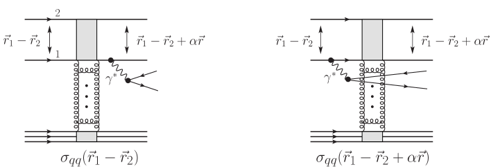
Figure 1: Leading order contribution to the diffractive Drell-Yan in the dipole-target collision.

Elastic dipole scattering depicted in Fig. 1 corresponds to forward scattering at small momentum transfers in the $t$-channel. In the leading order, the elastic scattering amplitude is given by one-loop diagram with two $t$-channel gluon exchanges. For on-shell intermediate spectators, corresponding four-dimensional loop integral can be reduced to two-dimensional one over the transverse momentum of one of the gluons

$$2i\mathrm{Im}\,F_{el}(\vec{\delta}_{\perp})=\int\frac{d^{2}k_{\perp}}{(2\pi)^{2}}\,A(\vec{k}_{\perp})A(\vec{\delta}_{\perp}-\vec{k}_{\perp}),\qquad\vec{\delta}_{\perp}\ll|\vec{k}_{\perp}|$$ (2)

where $A$ represents (inelastic) amplitude for one $t$-channel gluon exchange, and the last strong inequality guarantees that the proton target survives the scattering, hence, the elastic nature of the process. Then the convolution theorem of Fourier analysis leads to the optical theorem

$$\mathrm{Im}\,F_{el}(\vec{\delta})=\int d^{2}b\,e^{-i\vec{\delta}_{\perp}\cdot\vec{b}}\,\mathrm{Im}\,f_{el}(\vec{b}),\qquad 2i\mathrm{Im}\,f_{el}(\vec{b})=|\tilde{A}(\vec{b})|^{2}$$ (3)

In the case of multiple elastic rescattering, this relation leads to eikonalization of the bare elastic amplitude which then correctly takes into account gap survival effects. However, if one uses the elastic amplitude $f_{el}$ fitted to soft data, it must already contain the soft unitarity corrections, and one should include them twice as is sometimes done in the literature.

Straightforward calculations lead to $\bar{q}q$ dipole scattering amplitudes for $s$ and $u$-channel photon emission, respectively,

$$M^{(1)s}_{\bar{q}q}(\vec{b},\vec{r}_{p},\vec{r},\alpha) = -2ip_{i}^{0}\,\sqrt{4\pi}\,\frac{\sqrt{1-\alpha}}{\alpha^{2}}\,\Psi^{\mu}_{\gamma^{*}q}(\alpha,\vec{r})$$

$$\times\frac{1}{N_{c}}\sum_{X}\sum_{c_{f}c_{i}}\left(\big{|}V_{q}(\vec{b})-V_{q}(\vec{b}+\vec{r_{p}})\big{|}^{2}-\big{|}V_{q}(\vec{b}+\vec{r_{p}})\big{|}^{2}\right),$$

$$M^{(1)u}_{\bar{q}q}(\vec{b},\vec{r}_{p},\vec{r},\alpha) = 2ip_{i}^{0}\,\sqrt{4\pi}\,\frac{\sqrt{1-\alpha}}{\alpha^{2}}\,\Psi^{\mu}_{\gamma^{*}q}(\alpha,\vec{r})$$

$$\times\frac{1}{N_{c}}\sum_{X}\sum_{c_{f}c_{i}}\left(\big{|}V_{q}(\vec{b})-V_{q}(\vec{b}+\vec{r_{p}}+\alpha\vec{r})\big{|}^{2}-\big{|}V_{q}(\vec{b}+\vec{r_{p}}+\alpha\vec{r})\big{|}^{2}\right),$$

where the last terms subtract the contributions from diagrams corresponding to the situation when none of the gluons couple to the same quark line with the hard photon. Then, implied the fact that all fields disappear at infinite separations, i.e. $V_{q}(\vec{b})\to 0$ when $|\vec{b}|\to\infty$, we have due to antisymmetry of the integrand

$$\int d^{2}b\,e^{-i\vec{\delta}_{\perp}\cdot\vec{b}}\Big{[}\big{|}V_{q}(\vec{b}+\vec{r_{p}})\big{|}^{2n}-\big{|}V_{q}(\vec{b}+\vec{r_{p}}+\alpha\vec{r})\big{|}^{2n}\Big{]}\to 0,\quad n\geq 1\,,\quad|\vec{\delta}_{\perp}|\to 0\,,$$ (4)

such that these terms do not contribute to the final result. Using the optical theorem for the elastic amplitude

$$2i\,\mathrm{Im}\,f_{el}(\vec{b},\vec{r}_{p})=\frac{i}{N_{c}}\sum_{X}\sum_{c_{f}c_{i}}\,\big{|}V_{q}(\vec{b})-V_{q}(\vec{b}+\vec{r_{p}})\big{|}^{2},$$

we can finally write

$$M^{(1)}_{\bar{q}q}(\vec{b},\vec{r}_{p},\vec{r},\alpha)=-2ip_{i}^{0}\,\sqrt{4\pi}\,\frac{\sqrt{1-\alpha}}{\alpha^{2}}\,\Psi^{\mu}_{\gamma^{*}q}(\alpha,\vec{r})\left[2\mathrm{Im}\,f_{el}(\vec{b},\vec{r_{p}})-2\mathrm{Im}\,f_{el}(\vec{b},\vec{r}_{p}+\alpha\vec{r})\right]$$ (5)

i.e. the amplitude of the diffractive radiation is proportional to the difference between elastic amplitudes of the two Fock components, with and without the photon radiation. When a quark fluctuates into the upper Fock quark-photon state with the transverse separation $\vec{r}$, the final quark gets a transverse shift $\Delta\vec{r}=\alpha\vec{r}$. Then the quark dipoles with different sizes in the $|2q\rangle$ and $|2q\gamma^{*}\rangle$ components interact differently, and their difference corresponds to the diffractive Drell-Yan amplitude (5).

3 Diffractive Drell-Yan in proton-proton scattering

In the dipole picture, the typical enhanced Regge graphs correspond to elastic scattering of higher Fock states, which contain gluons, e.g. $|qqg\rangle$, $|qqgg\rangle$, etc. Note that in our approach we take into account the lowest Fock state $|qq\rangle$ contribution only. Such an approximation is justified for not very small fraction $x_{\gamma 1}=p_{\gamma}^{+}/p_{1}^{+}$ and scale $M^{2}$, where valence/sea quarks are dominated and the gluon contribution is rather small.

The total hadronic amplitude of the diffractive Drell-Yan process can be written as [1]

$$A_{if}=A^{(1)}_{if}+A^{(2)}_{if}+A^{(3)}_{if}\,,$$ (6)

where each term corresponds to $\gamma^{*}$ radiation by one of the valence (sea) quarks in the proton, in particular,

$$A^{(1)}_{if}(x_{\gamma 1},\vec{q}_{\perp},\lambda_{\gamma}) = \frac{i}{4}\,\alpha^{2}\int d^{2}r_{1}d^{2}r_{2}d^{2}r_{3}d^{2}rd^{2}bdx_{q_{1}}dx_{q_{2}}dx_{q_{3}}$$ (7)

$$\times \Psi_{i}(\vec{r}_{1},\vec{r}_{2},\vec{r}_{3};x_{q_{1}},x_{q_{2}},x_{q_{3}})\Psi_{f}^{*}(\vec{r}_{1}+\alpha\vec{r},\vec{r}_{2},\vec{r}_{3};x_{q_{1}}-x_{\gamma 1},x_{q_{2}},x_{q_{3}})$$

$$\times \Big{[}M^{\lambda_{\gamma}}_{\bar{q}q}(\vec{b},\vec{r}_{1}-\vec{r}_{2},\vec{r},\alpha)+M^{\lambda_{\gamma}}_{\bar{q}q}(\vec{b},\vec{r}_{1}-\vec{r}_{3},\vec{r},\alpha)\Big{]}e^{i\vec{l}_{\perp}\cdot\alpha\vec{r}}e^{i\vec{\delta}_{\perp}\cdot\vec{b}}$$

Here, $\lambda_{\gamma}=L,T$; $\vec{l}_{\perp}=\vec{\delta}_{\perp}-\vec{q}_{\perp}/\alpha$ ($z$-axis is directed along initial proton momentum); the hard photon with virtuality $q^{2}=M^{2}\gg m_{p}^{2}$, transverse $\vec{q}_{\perp}$ and fractional longitudinal $x_{\gamma 1}$ momenta is emitted from the first valence quark with impact parameter $\vec{r}_{1}$, other two valence quarks in the proton have impact parameters $\vec{r}_{2}$ and $\vec{r}_{3}$, respectively; $\vec{r}$ is transverse separation between the photon and the radiating quark; $\alpha=x_{\gamma 1}/x_{q_{1}}$ is the fraction of longitudinal momenta taken away by the photon from the radiating quark; $M^{L,T}_{\bar{q}q}$ are the Fourier-transformed amplitudes for the elastic quark dipole scattering off the proton target accompanied by the hard $L,T$-polarized photon emission; $\Psi_{i,f}$ are the light-cone wave functions of the $3q$ systems in the initial and final state, respectively. In Eq. (7) we implicitly assumed that exchanges $t$-channel gluons all together take a negligibly small longitudinal momentum compared to the collisions energy $\sqrt{s}$ and, hence, corrections to quark momenta due to gluon couplings are neglected in the wave functions.

The differential cross section for the single diffractive di-lepton production in the target rest frame reads

$$d^{\,8}\sigma^{sd}_{\lambda_{\gamma}}(pp\to pl^{+}l^{-}X) = \sum_{f}\sum_{n=1}^{3}|A^{(n)}_{if}(x_{\gamma 1},\vec{q}_{\perp},\lambda_{\gamma})|^{2}\frac{d\alpha}{\alpha(1-\alpha)}\frac{d^{2}q_{\perp}d^{2}\delta_{\perp}}{(2\pi)^{5}\,8(p_{i,n}^{0})^{2}}$$ (8)

$$\times \alpha_{em}\epsilon_{\mu}(\lambda_{\gamma})\epsilon^{*}_{\nu}(\lambda_{\gamma})L^{\mu\nu}\frac{dM^{2}d\Omega}{16\pi^{2}M^{4}},\quad\lambda_{\gamma}=L,T$$

where prefactors provide averaging over colors and helicities of exchanged $t$-channel gluons, $p_{i,n}^{0}$ is the energy of the radiating $n$th quark in the initial state, $n=1,\,...,\,3$; $\alpha_{em}=e^{2}/(4\pi)=1/137$ is the electromagnetic coupling constant. The second line in Eq.(8) describes decay of $\gamma^{*}$ into the leptonic pair $l^{+}l^{-}$ into solid angle $d\Omega=d\phi d\cos\theta$, and $L^{\mu\nu}$ is the standard leptonic tensor. We keep in the cross section only diagonal in the photon polarization $\lambda_{\gamma}=L,T$ terms (non-diagonal ones drop out after integration over leptonic azimuthal angle $\phi$). Integrating the diffractive differential DY cross section over the photon transverse momentum $\vec{q}_{\perp}$ we get

$$\frac{d^{4}\sigma_{L,T}(pp\to pl^{+}l^{-}X)}{d\ln\alpha\,dM^{2}\,d^{2}\delta_{\perp}}=\frac{\alpha_{em}}{3\pi M^{2}}\,\frac{d^{3}\sigma_{L,T}(pp\to p\gamma^{*}X)}{d\ln\alpha\,d^{2}\delta_{\perp}}\,.$$ (9)

Then applying the completeness relation

$$\sum_{f}\Psi_{f}(\vec{r}_{1}+\alpha\vec{r},\vec{r}_{2},\vec{r}_{3};x_{q_{1}},x_{q_{2}},x_{q_{3}})\Psi^{*}_{f}(\vec{r}\,^{\prime}_{1}+\alpha\vec{r}\,^{\prime},\vec{r}\,^{\prime}_{2},\vec{r}\,^{\prime}_{3};x^{\prime}_{q_{1}},x^{\prime}_{q_{2}},x^{\prime}_{q_{3}})$$

$$\phantom{.......}=\,\delta(\vec{r}_{1}-\vec{r}\,^{\prime}_{1}+\alpha(\vec{r}-\vec{r}\,^{\prime}))\delta(\vec{r}_{2}-\vec{r}\,^{\prime}_{2})\delta(\vec{r}_{3}-\vec{r}\,^{\prime}_{3})\prod_{j=1}^{3}\delta(x_{q_{j}}-x^{\prime}_{q_{j}})$$ (10)

we get the diffractive $\gamma^{*}$ production cross section in the following differential form

$$\frac{d^{3}\sigma_{\lambda_{\gamma}}(pp\to p\gamma^{*}X)}{d\ln\alpha\,d^{2}\delta_{\perp}}=\frac{\sum_{q}Z_{q}^{2}}{64\pi^{2}}\int d^{2}r_{1}d^{2}r_{2}d^{2}r_{3}d^{2}r\,d^{2}bd^{2}b^{\prime}\,dx_{q_{1}}dx_{q_{2}}dx_{q_{3}}$$

$$\qquad\qquad\times\,|\tilde{\Psi}^{\lambda_{\gamma}}_{\gamma^{*}q}(\alpha,\vec{r})|^{2}|\Psi_{i}(\vec{r}_{1},\vec{r}_{2},\vec{r}_{3};x_{q_{1}},x_{q_{2}},x_{q_{3}})|^{2}$$

$$\qquad\qquad\times\,\Delta(\vec{r}_{1},\vec{r}_{2},\vec{r}_{3};\vec{b};\vec{r},\alpha)\Delta(\vec{r}_{1},\vec{r}_{2},\vec{r}_{3};\vec{b}\,^{\prime};\vec{r},\alpha)\,e^{i\vec{\delta}_{\perp}\cdot(\vec{b}-\vec{b}\,^{\prime})}$$ (11)

where $\tilde{\Psi}_{\gamma^{*}q}=\Psi_{\gamma^{*}q}/Z_{q}$, and

$$\Delta = -2\mathrm{Im}\,f^{\mathrm{KST}}_{el}(\vec{b},\vec{r}_{1}-\vec{r}_{2})+2\mathrm{Im}\,f^{\mathrm{KST}}_{el}(\vec{b},\vec{r}_{1}-\vec{r}_{2}+\alpha\vec{r})$$ (12)

$$-2\mathrm{Im}\,f^{\mathrm{KST}}_{el}(\vec{b},\vec{r}_{1}-\vec{r}_{3})+2\mathrm{Im}\,f^{\mathrm{KST}}_{el}(\vec{b},\vec{r}_{1}-\vec{r}_{3}+\alpha\vec{r})\,,$$

where the Kopeliovich-Schäfer-Tarasov (KST) parameterization of the elastic dipole-target amplitude fitted to the soft data [9, 10, 11] and, hence, valid at $|\vec{r}_{i}-\vec{r}_{j}|\sim\vec{b},\,i\not=j$ is used. Finally, going over to the forward limit $\vec{\delta}_{\perp}=0$ we obtain

$$\frac{d^{3}\sigma_{\lambda_{\gamma}}(pp\to p\gamma^{*}X)}{d\ln\alpha\,d\delta_{\perp}^{2}}\Big{|}_{\delta_{\perp}=0}=\frac{\sum_{q}Z_{q}^{2}}{64\pi}\int d^{2}r_{1}d^{2}r_{2}d^{2}r_{3}d^{2}r\,dx_{q_{1}}dx_{q_{2}}dx_{q_{3}}$$

$$\qquad\times\,|\tilde{\Psi}^{\lambda_{\gamma}}_{\gamma^{*}q}(\alpha,\vec{r})|^{2}|\Psi_{i}(\vec{r}_{1},\vec{r}_{2},\vec{r}_{3};x_{q_{1}},x_{q_{2}},x_{q_{3}})|^{2}\,\left[\int d^{2}b\,\Delta(\vec{r}_{1},\vec{r}_{2},\vec{r}_{3};\vec{b};\vec{r},\alpha)\right]^{2}$$ (13)

We see that normalization of the cross section agrees with the original result of Ref. [1]. The total diffractive cross section is then given by

$$\frac{d\sigma(pp\to p\gamma^{*}X)}{d\ln\alpha}=\frac{1}{B_{sd}^{DY}(s)}\frac{d^{3}\sigma(pp\to p\gamma^{*}X)}{d\ln\alpha\,d\delta_{\perp}^{2}}\Big{|}_{\delta_{\perp}=0}$$ (14)

where $B_{sd}^{DY}(s)$ is the diffractive slope similar to the one measured in diffractive DIS.

The next step is to introduce the proton wave function assuming the Gaussian shape for the quark distributions in the proton as

$$|\Psi_{i}(\vec{r}_{1},\vec{r}_{2},\vec{r}_{3};x_{q_{1}},x_{q_{2}},x_{q_{3}})|^{2} = \frac{2+a/b}{\pi^{2}ab}\exp\Big{[}-\frac{r_{1}^{2}}{a}-\frac{r_{2}^{2}+r_{3}^{2}}{b}\Big{]}\rho(x_{q_{1}},x_{q_{2}},x_{q_{3}})$$ (15)

$$\times \delta(\vec{r}_{1}+\vec{r}_{2}+\vec{r}_{3})\delta(1-x_{q_{1}}-x_{q_{2}}-x_{q_{3}})$$

where $a=\langle r_{\bar{q}q}^{2}\rangle$ and $b=\langle R_{q}^{2}\rangle$ are the diquark mean radius squared and the quark mean distance from the diquark squared, respectively. In this work, we will use the simplest case of symmetric valence quarks distribution assuming that $r_{\bar{q}q}=R_{q}=0.85$ fm.

Then valence quark distribution in the proton is given by

$$\int dx_{q_{2}}dx_{q_{3}}\rho(x_{q_{1}},x_{q_{2}},x_{q_{3}})=\rho_{q_{1}}(x_{q_{1}})\,.$$

where we integrated out the longitudinal fractions of the diquark in the proton. Generalization of the three-body proton wave function (15) including different quark and antiquark flavors, as well as sea quarks, leads to the proton structure function [12]

$$\sum_{q}Z_{q}^{2}[\rho_{q}(x_{q})+\rho_{\bar{q}}(x_{q})]=\frac{1}{x_{q}}F_{2}(x_{q}),\qquad x_{q}=\frac{x_{\gamma 1}}{\alpha}\,.$$ (16)

4 Numerical results for differential DDY cross sections

In Fig. 2 the ratio of the diffractive to inclusive DY cross sections is plotted as a function of di-lepton invariant mass squared $M^{2}$ (left panel) and photon fractional light-cone momentum $x_{\gamma 1}$ (right panel) at different energies. In the left panel, the curves are given for fixed $x_{\gamma 1}=0.5$ (solid lines) and $x_{\gamma 1}=0.9$ (dashed lines). In the right panel, the curves are given for fixed $M^{2}=50\,\textrm{GeV}^{2}$ (solid lines) and $M^{2}=500\,\textrm{GeV}^{2}$ for $\sqrt{s}=14$ TeV and 500 GeV, and $M^{2}=200\,\textrm{GeV}^{2}$ at $\sqrt{s}=40$ GeV (dashed lines). The pairs of solid/dashed curves in the both panels correspond to $\sqrt{s}=40\,\textrm{GeV}$, $500$ GeV and $14$ TeV from top to bottom, respectively. Here we used the KST parameterization for the dipole-target scattering amplitude [10, 9, 11] and $F_{2}$ parameterization by Cudell and Soyez [13] are used here. In this calculation we consider the unpolarized case summing up the contributions of longitudinal and transverse parts both in the diffractive and inclusive cross sections.

Figure 2: The ratio of the diffractive to inclusive Drell-Yan cross sections as function of the lepton-pair invariant mass squared $M^{2}$ (left panel) and photon fraction $x_{\gamma 1}$ (right panel) at different energies.

As seen from Fig. 2, the DDY-to-DY cross section ratio is falling with energy. However, naively one could expect basing on QCD factorisation, that the DDY cross section, which is proportional to the dipole cross section squared, should rise with energy steeper than the total inclusive cross section. At the same time, the ratio rises with the hard scale of the process, $M^{2}$. This also looks counterintuitive, since diffraction is usually associated with soft interactions [14]. These effects are different from ones emerging in Regge factorisation-based calculations, where we observe a slow rise of the DDY-to-DY cross section ratio with c.m.s. energy and its practical independence on the hard scale of the process $M^{2}$ [15].

In order to understand such an interesting behavior of the DDY-to-DY cross sections ratio obtained in the color dipole approach, let us look at the amplitude of the DDY process, which is proportional to the difference between the dipole cross sections of the Fock states with and without the hard photon emission [1], i.e.

$$M_{DDY}\sim\sigma(\vec{R})-\sigma(\vec{R}-\alpha\vec{r})=\frac{2\alpha\sigma_{0}}{R_{0}^{2}(x)}e^{R^{2}/R_{0}^{2}(x)}\,\left(\vec{r}\cdot\vec{R}\right)+h.o.$$ (17)

assuming the simplest Golec-Biernat-Wusthoff (GBW) slope for the dipole cross section [16], and the hardness of the emitted photon implies $r\sim 1/M\ll R_{0}(x)$. We see now that the diffractive DY amplitude is linear in $r$, so the diffractive cross section turns out to be a quadratic function of $r$, which is different from e.g. the diffractive DIS process where the cross section is proportional to $r^{4}$ and is dominated by soft fluctuations (see e.g. Refs. [6, 7]). Since the diffractive DY cross section is proportional to $r^{2}$, then soft and hard interactions contribute on the same footing [1], which is one of the basic sources of the QCD factorisation breaking in diffractive DY process.

Figure 3: Diffractive Drell-Yan cross section (in fb) as function of the lepton-pair invariant mass squared $M^{2}$ (left panel) and photon fraction $x_{\gamma 1}$ (right panel) at the RHIC II c.m.s. energy $\sqrt{s}=500$ GeV.

We also compare predictions for the diffractive DY cross section for different parameterizations for elastic dipole-target scattering amplitude corresponding to scattering of small (GBW given by Refs. [16, 9, 17]) and large (KST given by Refs. [9, 10, 11]) dipoles. As an example, in Fig. 3 we present the diffractive Drell-Yan cross section as function of the lepton-pair invariant mass squared $M^{2}$ (left panel) and photon fraction $x_{\gamma 1}$ (right panel) at the RHIC II c.m.s. energy $\sqrt{s}=500$ GeV. We notice that the GBW parameterization leads to roughly a factor of two smaller cross section than the one obtained with the KST parameterization, however, both of them exhibit basically the same $x_{\gamma 1}$ and $M^{2}$ shapes. It means that the evolution of the dipole size can only affect the overall normalization of the DDY cross section. Since arguments in the elastic amplitude $f_{el}({\vec{r}}_{p},{\vec{b}})$, the impact distance between the target and the projectile $b$ and the transverse distance between projectile quarks $r_{p}\sim|\vec{r}_{i}-\vec{r}_{j}|,\,i\not=j$, are of the same order and given at the soft hadronic scale, then the use of KST parameterization fitted to the soft hadron scattering data data is justified in the case of diffractive DY.

5 Conclusion

The QCD factorisation breaking effects in the diffractive Drell-Yan process lead to quite different properties of the corresponding observables with respect to QCD factorisation-based calculations. A quark cannot diffractively radiate a photon in the forward direction, whereas a hadron can due to the presence of transverse motion of spectator quarks in the projectile hadron. For this reason, the diffractive DY cross section depends on the hadronic size explicitly breaking the QCD factorisation.

This leads to the physical picture where hard and soft interactions are equally important for DY diffraction, and their relative contributions are independent of the hard scale, like in the inclusive DY process. This is a result of the specific property of DY diffraction: its cross section is a linear, rather than quadratic function of the dipole cross section. On the contrary, diffractive DIS is predominantly a soft process, because its cross section is proportional to the dipole cross section squared.

Contrary to what follows from the calculations based on QCD factorisation, the ratio of the diffractive to inclusive cross sections falls with energy, but rises with the di-lepton effective mass $M$. This happens due to the saturated behavior of the dipole cross section which levels off at large separations. All these properties are different from those in the diffractive DIS process, where QCD factorisation is exact. In addition, we made predictions for the differential (in photon fractional momentum $x_{\gamma 1}$ and di-lepton invariant mass squared $M^{2}$) cross sections for the diffractive DY process at the energies of RHIC (500 GeV) and LHC (14 TeV).

5.1 Acknowledgments

Useful discussions and helpful correspondence with Jochen Bartels, Antoni Szczurek, Gunnar Ingelman and Mark Strikman are gratefully acknowledged. This study was partially supported by the Carl Trygger Foundation (Sweden), by Fondecyt (Chile) grant 1090291, and by Conicyt-DFG grant No. 084-2009. Authors are also indebted to the Galileo Galilei Institute of Theoretical Physics (Florence, Italy) and to the INFN for partial support and warm hospitality during completion of this work.

References

References

- [1] B. Z. Kopeliovich, I. K. Potashnikova, I. Schmidt, A. V. Tarasov, Phys. Rev. D74, 114024 (2006) [hep-ph/0605157].
- [2] B. Z. Kopeliovich, I. K. Potashnikova, I. Schmidt, A. V. Tarasov, Phys. Rev. D76, 034019 (2007) [hep-ph/0702106].
- [3] R. J. Glauber, Phys. Rev. 100, 242 (1955).
- [4] E. Feinberg and I. Ya. Pomeranchuk, Nuovo. Cimento. Suppl. 3 (1956) 652.
- [5] M. L. Good and W. D. Walker, Phys. Rev. 120 (1960) 1857.
- [6] B. Z. Kopeliovich, I. K. Potashnikova, I. Schmidt, Braz. J. Phys. 37, 473-483 (2007). [arXiv:hep-ph/0604097 [hep-ph]].
- [7] B. Z. Kopeliovich and B. Povh, Z. Phys. A356, 467 (1997).
- [8] B. Z. Kopeliovich, I. K. Potashnikova, I. Schmidt, M. Siddikov, Phys. Rev. C84, 024608 (2011) [arXiv:1105.1711 [hep-ph]].
- [9] B. Z. Kopeliovich, A. H. Rezaeian, I. Schmidt, Phys. Rev. D78, 114009 (2008) [arXiv:0809.4327 [hep-ph]].
- [10] B. Z. Kopeliovich, I. K. Potashnikova, I. Schmidt and J. Soffer, Phys. Rev. D 78, 014031 (2008) [arXiv:0805.4534 [hep-ph]].
-
[11]
B. Z. Kopeliovich, A. Schäfer and A. V. Tarasov, Phys. Rev. D62, 054022 (2000) [arXiv:hep-ph/9908245];
B. Z. Kopeliovich, I. K. Potashnikova, I. Schmidt, J. Soffer, Phys. Rev. D78, 014031 (2008) [arXiv:0805.4534 [hep-ph]]. - [12] B. Z. Kopeliovich, J. Raufeisen, A. V. Tarasov, Phys. Lett. B503, 91-98 (2001). [hep-ph/0012035].
- [13] J. R. Cudell, G. Soyez, Phys. Lett. B516, 77-84 (2001). [hep-ph/0106307].
- [14] B. Z. Kopeliovich, proc. of the workshop Hirschegg 95: Dynamical Properties of Hadrons in Nuclear Matter, Hirschegg January 16-21, 1995, ed. by H. Feldmeyer and W. Nörenberg, Darmstadt, 1995, p. 102 [hep-ph/9609385].
- [15] G. Kubasiak, A. Szczurek, Phys. Rev. D84, 014005 (2011). [arXiv:1103.6230 [hep-ph]].
- [16] K. J. Golec-Biernat, M. Wusthoff, Phys. Rev. D59, 014017 (1998). [hep-ph/9807513].
- [17] B. Z. Kopeliovich, H. J. Pirner, A. H. Rezaeian and I. Schmidt, Phys. Rev. D77, 034011 (2008) [arXiv:0711.3010 [hep-ph]].