Drell-Yan diffraction: breakdown of QCD factorisation

Abstract

We consider the diffractive Drell-Yan process in proton-(anti)proton collisions at high energies in the color dipole approach. The calculations are performed at forward rapidities of the leptonic pair. Effect of eikonalization of the universal “bare” dipole-target elastic amplitude in the saturation regime takes into account the principal part of the gap survival probability. We present predictions for the total and differential cross sections of the single diffractive lepton pair production at RHIC and LHC energies. We analyze implications of the QCD factorisation breakdown in the diffractive Drell-Yan process, which is caused by a specific interplay of the soft and hard interactions, and resulting in rather unusual properties of the corresponding observables.

I Introduction

The exclusive diffractive production of particles in hadron-hadron scattering at high energies is one of the basic tools for both experimental and theoretical studies of the small-$x$ and nonperturbative QCD physics. The understanding of the mechanisms of inelastic diffraction came with the pioneering works of Glauber Glauber , Feinberg and Pomeranchuk FP56 , Good and Walker GW . If the incoming plane wave contains components interacting differently with the target, the outgoing wave will have a different composition, i.e. besides elastic scattering a new diffractive state will be created (for a detailed review on QCD diffraction, see Ref. KPSdiff ). Among the most important examples, the leading twist diffractive Drell-Yan (DDY) process is of a special interest since it gives rise to a clean experimental signature for the QCD factorisation breaking effects where soft and hard interactions interplay with each other KPST06 , thus, providing an access to the soft QCD physics RP11 .

Typically, the single-diffractive Drell-Yan reaction in $pp$ collisions is characterized by a relatively small momentum transfer between the colliding protons, such that one of them, e.g. $p_{1}$, radiates a hard virtual photon $k^{2}=M^{2}\gg m_{p}^{2}$ and hadronizes into a hadronic system $X$ both moving in forward direction and separated by a large rapidity gap from the second proton $p_{2}$, which remains intact, i.e.

$$p_{1}+p_{2}\to\gamma^{*}(l^{+}l^{-})+X+(gap)+p_{2}$$ (1)

Both the di-lepton and $X$, the debris of $p_{1}$, stay in the forward fragmentation region. In this case, the virtual photon is predominantly emitted by the valence quarks of the proton $p_{1}$. Below we will refer to this as the diffractive Drell-Yan process at forward rapidities. Notice that this is different from double diffractive Drell-Yan process, where the di-lepton $l^{+}l^{-}$ is produced at central rapidities, while both protons survive the collision (see e.g. Ref. Antoni11 ). Then, the $\gamma^{*}$ can be emitted by a sea quark or antiquark. We postpone this case for future studies, and concentrate here on the single diffractive Drell-Yan process.

In some of previous studies Refs. Antoni11 ; Landshoff-DDY of the single diffractive Drell-Yan reaction the analysis was made within the phenomenological Pomeron-Pomeron and $\gamma$-Pomeron fusion mechanisms using the Ingelman-Shlein approach ISh based on QCD and Regge factorization. This led to specific features of the differential cross sections similar to those in diffractive DIS process, e.g., a slow increase of the diffractive-to-inclusive DY cross sections ratio with c.m.s. energy $\sqrt{s}$, its practical independence on the hard scale, the invariant mass of the lepton pair squared, $M^{2}$ Antoni11 .

Differently, the study of the diffractive Drell-Yan reaction performed in KPST06 within the light-cone dipole description revealed importance of soft interactions with the partons spectators, which contributes on the same footing as hard perturbative ones, and strongly violate QCD factorization.

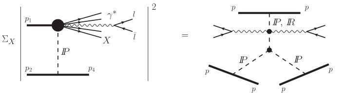
Figure 1: The cross section of the diffractive DY process summed over all excitation channels at fixed effective mass $M_{X}$ (left panel) corresponding to the Mueller graph in Regge picture (right panel).

Absorptive corrections are normally associated with the soft interactions between target and projectile, and they play an important role in diffractive hadron-hadron scattering. One can derive a Regge behavior of the diffractive cross section of heavy photon production in terms of the usual light-cone variables,

$$x_{\gamma 1}=\frac{p_{\gamma}^{+}}{p_{1}^{+}};\ \ \ \ \ x_{\gamma 2}=\frac{p_{\gamma}^{-}}{p_{2}^{-}},$$ (2)

so that $x_{\gamma 1}x_{\gamma 2}=(M^{2}+k_{T}^{2})/s$ and $x_{\gamma 1}-x_{\gamma 2}=x_{\gamma F}$, where $M$, $k_{T}$ and $x_{\gamma F}$ are the invariant mass, transverse momentum and Feynman $x_{F}$ of the heavy photon (di-lepton). n the limit of small $x_{\gamma 1}\to 0$ and large $z_{p}\equiv p_{4}^{+}/p_{2}^{+}\to 1$ the diffractive DY cross section is given by the Mueller graph shown in Fig. 1. In this case, the end-point behavior is dictated by the following general result

$$\frac{d\sigma}{dz_{p}dx_{\gamma 1}dt}\Big{|}_{t\to 0}\propto\frac{1}{(1-z_{p})^{2\alpha_{{I\!\!P}}(t)-1}x_{\gamma 1}^{\varepsilon}}\,,$$ (3)

where $\alpha_{{I\!\!P}}(t)$ is the Pomeron trajectory corresponding to the $t$-channel exchange, and $\varepsilon$ is equal to 1 or 1/2 for the Pomeron ${I\!\!P}$ or Reggeon ${I\!\!R}$ exchange corresponding to $\gamma^{*}$ emission from sea or valence quarks, respectively (see Fig. 1).

As an alternative to the factorization based QCD approach, the dipole description of the QCD diffraction, was presented in Refs. KLZ81 (see also Ref. BBGG81 ). It is based on the fact that dipoles of different transverse size $r_{\perp}$ interact with different cross sections $\sigma(r_{\perp})$, leading to the single inelastic diffractive scattering with a cross section, which in the forward limit is given by KLZ81 ,

$$\frac{\sigma_{sd}}{dp_{\perp}^{2}}\Bigg{|}_{p_{\perp}=0}=\frac{\langle\sigma^{2}(r_{\perp})\rangle-\langle\sigma(r_{\perp})\rangle^{2}}{16\pi},\,$$ (4)

where $p_{\perp}$ is the transverse momentum of the recoil proton, $\sigma(r_{\perp})$ is the universal dipole-proton cross section, and operation $\langle...\rangle$ means averaging over the dipole separation.

The color dipole description of Drell-Yan inclusive process first introduced in Ref. deriv1 (see also Ref. BHQ ), treats the production of a heavy di-lepton like photon bremsstrahlung, rather than $\bar{q}q$ annihilation. Such a difference is a consequence of Lorentz non-invariance of the space-time description of the interaction, which varies with the reference frame. Only observables must be Lorentz-invariant.

The dipole approach applied to diffractive Drell-Yan reaction in Ref. KPST06 , led to the QCD factorisation breaking, which manifests itself in specific features like a significant damping of the cross section at high $\sqrt{s}$ compared to the inclusive DY case. This is rather unusual, since a diffractive cross section, which is proportional to the dipole cross section squared, could be expected to rise with energy steeper than the total inclusive cross section, like it occurs in the diffractive DIS process. At the same time, the ratio of the DDY to DY cross sections was found in Ref. KPST06 to rise with the hard scale, $M^{2}$. This is also in variance with diffraction in DIS, which is associated with the soft interactions BP97 ; ourDDIS .

The absorptive corrections affect differently the diagonal and off-diagonal terms in the hadronic current PCAC , in opposite directions, leading to an unavoidable breakdown of the QCD factorisation in processes with off-diagonal contributions only. Namely, the absorptive corrections enhance the diagonal terms at larger $\sqrt{s}$, whereas they strongly suppress the off-diagonal ones. In the diffractive DY process a new state, the heavy lepton pair, is produced, hence, the whole process is of entirely off-diagonal nature, whereas in the diffractive DIS contains both diagonal and off-diagonal contributions KPSdiff . This is the first reason why the QCD factorisation is broken in the DDY reaction.

The second reason of the QCD factorisation breaking is more specific and concerns the interplay of soft and hard interactions in the DDY amplitude. In particular, this leads to the leading twist nature of the DDY process, whereas DDIS is of the higher twist KPST06 . Large and small size projectile fluctuations contribute to the diffractive DY process at the same footing, which further deepens the dramatic breakdown of the QCD factorisation in DDY. We will shortly discuss this issue below when presenting the numerical results.

Quasieikonal model KMR for the so-called “enhanced” probability $\hat{S}_{enh}$ (see e.g. Refs. enh-1 ; enh-2 ), frequently used to describe the QCD factorisation breaking in diffractive processes, is not well justified in higher orders, whereas the color dipole approach considered here, correctly includes all diffraction excitations to all orders KPSdiff .

In this work, we investigate further the unusual features of the Drell-Yan diffraction KPST06 in the framework of the color dipole approach. We show that the unitarization effects can be correctly taken into account through eikonalization of the universal “bare” elastic dipole-target amplitude. This generalized dipole approach pretends to take into account the soft absorptive effects on the same footing with the hard dipole-target scattering. Such effects are included into the phenomenological partial elastic dipole amplitude fitted to data. This allows to predict the diffractive DY cross section completely in terms of the single parameterization of the dipole cross section known independently from the soft hadron scattering data.

The paper is organized as follows. Section II contains derivation of the diffractive Drell-Yan amplitude in the dipole approach. Section III is devoted to a discussion of the unitarity corrections through the eikonalization of the elastic “bare” dipole-target scattering amplitude. In Section IV a short overview of different parameterizations of the elastic dipole-target scattering amplitude for small and large dipoles is given. The formulae for the single diffractive Drell-Yan cross section are explicitly derived in Section V. Discussion of numerical results for the differential distributions and basic features of the diffractive DY is presented in Section VI. Finally, Section VII with the summary and conclusions closes our paper.

II Diffractive Drell-Yan amplitude in the dipole approach

In the forward limit $p_{T}=0$, the photon radiation from a quark in inelastic collisions vanishes which was explained at the intuitive level, as well as demonstrated by a direct calculation of Feynman graphs in Ref. KST99 . The same is also true for forward diffraction proceeding via gluon pair exchange (in the color singlet state) with no momentum transfer between the projectile quark and the proton target KPST06 . Disappearance of both inelastic and diffractive forward photon radiation happens due to the fact that if the electric charge gets no “kick”, i.e. is not accelerated, no photon is radiated, provided that the radiation time considerably exceeds the duration time of interaction. This is dictated by the renown Landau-Pomeranchuk principle LP : radiation depends on the strength of the accumulated kick, rather than on its structure, if the time scale of the kick is shorter than the radiation time.

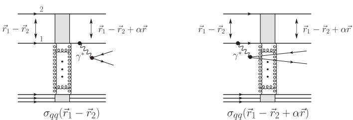
Figure 2: Leading order contribution to the diffractive Drell-Yan in the dipole-target collision.

The non-Abelian case, QCD, is different: a quark can radiate gluons diffractively in the forward direction. This happens due to possibility of interaction between the radiated gluon and the target. Such a process, in particular, is very important for diffractive heavy flavor production heavyF .

Notice that the disappearance of Abelian radiation is only true for the diffractive scattering of a single quark off the target, and it does not hold for diffractive hadron-hadron scattering. As was demonstrated in Ref. KPST06 , due to the internal transverse motion of the valence quarks inside the proton, which corresponds to finite large transverse separations between them, the forward photon radiation does not vanish. This means that even at a hard scale the Abelian radiation is sensitive to the hadron size due to a dramatic break down of QCD factorization DL88 . It was firstly found in Refs. Collins93 ; Collins97 that factorization for diffractive Drell-Yan reaction fails due to the presence of spectator partons in the Pomeron. In Ref. KPST06 it was demonstrated that factorization in Drell-Yan diffraction is even more broken due to presence of spectator partons in the colliding hadrons.

As usual, we work in the rest frame of the target proton which remains intact after the collision. The hard part of the Drell-Yan process is given by the inelastic amplitude of $\gamma^{*}$ radiation by a projectile quark (valence or sea) due to its interaction with the target through a gluon exchange as shown in Fig. 2. It consists of two terms corresponding to interaction of two different Fock states with the target – a bare quark before the photon emission $|q\rangle$ ($s$-channel diagram), and a quark accompanied by a Weizäcker-Williams photon $|q\gamma^{*}\rangle$ ($u$-channel diagram).

Let us consider first heavy photon bremsstrahlung by quark scattered off the proton target. We imply that the longitudinal momentum of the projectile quark cannot be changed significantly at high energies. In the high energy limit the corresponding $s$ and $u$-channel contributions can be written as follows deriv1 ; RPN02

$${\cal M}^{\mu}_{s}\simeq-iZ_{q}e\,\alpha(1-\alpha)\sum_{\sigma}\frac{{\bar{u}}_{\sigma_{f}}(p_{f})\gamma^{\mu}u_{\sigma}(p_{f}+q)}{\alpha^{2}l_{\perp}^{2}+\eta^{2}}\,{\cal A}_{\sigma\sigma_{i}}(k_{\perp}),$$

$${\cal M}^{\mu}_{u}\simeq iZ_{q}e\,\alpha\sum_{\sigma}\frac{{\bar{u}}_{\sigma}(p_{i}-q)\gamma^{\mu}u_{\sigma_{i}}(p_{i})}{\alpha^{2}(\vec{l}_{\perp}+\vec{k}_{\perp})^{2}+\eta^{2}}\,{\cal A}_{\sigma\sigma_{f}}(k_{\perp}),\quad\eta^{2}=(1-\alpha)M^{2}+\alpha^{2}m_{q}^{2}$$ (5)

where $\vec{k}_{\perp}=\vec{p}_{f\perp}+\vec{q}_{\perp}-\vec{p}_{i\perp}$ is the transverse momentum of exchanged gluon, and $\vec{l}_{\perp}=\vec{p}_{f\perp}-(1-\alpha)\vec{q}_{\perp}/\alpha$ is the transverse momentum of the final quark in a frame where $z$-axis is parallel to the photon momentum, and the amplitude for scattering of a quark off a nucleon in the rest frame of the nucleon reads

$${\cal A}_{\sigma\sigma_{i}}(\vec{k}_{\perp})\simeq 2p_{i}^{0}\delta_{\sigma\sigma_{i}}{\cal V}_{q}(\vec{k}_{\perp}),\qquad{\cal A}_{\sigma\sigma_{f}}(\vec{k}_{\perp})\simeq 2p_{f}^{0}\delta_{\sigma\sigma_{f}}{\cal V}_{q}(\vec{k}_{\perp})$$

Finally, we can switch to impact parameter space performing the Fourier transformation over $\vec{l}_{\perp}$ and $\vec{k}_{\perp}$ and write down the total amplitude for the photon radiation in inelastic quark-proton scattering

$$M_{q}(\vec{b},\vec{r})=-2ip_{i}^{0}\,\sqrt{4\pi}\,\frac{\sqrt{1-\alpha}}{\alpha^{2}}\,\Psi^{\mu}_{\gamma^{*}q}(\alpha,\vec{r})\cdot\Big{[}V_{q}(\vec{b})-V_{q}(\vec{b}+\alpha\vec{r})\Big{]},$$

$$V_{q}(\vec{b})=\int\frac{d^{2}k_{\perp}}{(2\pi)^{2}}e^{-i\vec{k}_{\perp}\cdot\vec{b}}{\cal V}_{q}(\vec{k}_{\perp})\,,$$

where $\alpha\vec{r}$ corresponds to the transverse separation between initial and final quark induced by the hard photon radiation, and $\Psi^{\mu}_{\gamma^{*}q}(\alpha,\vec{r})$ is the light-cone wave function of the $q\to\gamma^{*}q$ transition in the mixed representation defined as follows

$$\Psi^{\mu}_{\gamma^{*}q}(\alpha,\vec{r})=Z_{q}\sqrt{\alpha_{em}}\,\alpha^{3}\sqrt{1-\alpha}\int\frac{d^{2}l_{\perp}}{(2\pi)^{2}}e^{-i\vec{l}_{\perp}\cdot\alpha\vec{r}}\,\frac{{\bar{u}}_{\sigma_{f}}(p_{f})\gamma^{\mu}u_{\sigma}(p_{f}+q)}{\alpha^{2}l_{\perp}^{2}+\eta^{2}}$$

The explicit expressions of the LC wave functions products for radiation of longitudinally ($\lambda=0$) and transversely ($\lambda=\pm 1$) polarized photons are deriv1 ; BHQ ; deriv2

$$\Psi^{T}_{\gamma^{*}q}(\alpha,\vec{\rho}_{1})\Psi^{T*}_{\gamma^{*}q}(\alpha,\vec{\rho}_{2})=\sum_{\lambda=\pm 1}\frac{1}{2}\sum_{\sigma_{f}\sigma_{i}}\epsilon^{*}_{\mu}(\lambda)\Psi^{\mu}_{\gamma^{*}q}(\alpha,\vec{\rho}_{1})\epsilon_{\nu}(\lambda)\Psi^{\nu*}_{\gamma^{*}q}(\alpha,\vec{\rho}_{2})$$

$$\qquad=Z_{q}^{2}\frac{\alpha_{em}}{2\pi^{2}}\Bigg{\{}m_{q}^{2}\alpha^{4}{\rm K}_{0}\left(\eta\rho_{1}\right){\rm K}_{0}\left(\eta\rho_{2}\right)+\left[1+\left(1-\alpha\right)^{2}\right]\eta^{2}\frac{\vec{\rho}_{1}\cdot\vec{\rho}_{2}}{\rho_{1}\rho_{2}}{\rm K}_{1}\left(\eta\rho_{1}\right){\rm K}_{1}\left(\eta\rho_{2}\right)\Bigg{\}},$$

$$\Psi^{L}_{\gamma^{*}q}(\alpha,\vec{\rho}_{1})\Psi^{L*}_{\gamma^{*}q}(\alpha,\vec{\rho}_{2})=\frac{1}{2}\sum_{\sigma_{f}\sigma_{i}}\epsilon^{*}_{\mu}(\lambda=0)\Psi^{\mu}_{\gamma^{*}q}(\alpha,\vec{\rho}_{1})\epsilon_{\nu}(\lambda=0)\Psi^{\nu*}_{\gamma^{*}q}(\alpha,\vec{\rho}_{2})$$

$$\qquad=Z_{q}^{2}\frac{\alpha_{em}}{\pi^{2}}M^{2}\left(1-\alpha\right)^{2}{\rm K}_{0}\left(\eta\rho_{1}\right){\rm K}_{0}\left(\eta\rho_{2}\right).$$

Now let us turn to elastic dipole scattering as depicted in Fig. 2. It corresponds to forward scattering at small momentum transfers in the $t$-channel. Generally speaking, $\sqrt{-t}\to\Lambda_{QCD}$ corresponds to the physical forward scattering limit since transverse momentum of a proton in the final state cannot be resolved to a better accuracy than its inverse size.

In the leading order the elastic scattering amplitude is given by one-loop diagram with two $t$-channel gluon exchanges. Due to on-shell intermediate spectators, corresponding four-dimensional loop integral can be reduced to two-dimensional one over the transverse momentum of one of the gluons

$$2i\mathrm{Im}\,F_{el}(\vec{\delta}_{\perp})=\int\frac{d^{2}k_{\perp}}{(2\pi)^{2}}\,A(\vec{k}_{\perp})A(\vec{\delta}_{\perp}-\vec{k}_{\perp}),\qquad\vec{\delta}_{\perp}\ll|\vec{k}_{\perp}|$$ (6)

where $A$ represents (inelastic) amplitude for one $t$-channel gluon exchange, and the last strong inequality guarantees that the proton target survives the scattering, hence, the elastic nature of the process. Then the convolution theorem of Fourier analysis leads to the optical theorem

$$\mathrm{Im}\,F_{el}(\vec{\delta})=\int d^{2}b\,e^{-i\vec{\delta}_{\perp}\cdot\vec{b}}\,\mathrm{Im}\,f_{el}(\vec{b}),\qquad 2i\mathrm{Im}\,f_{el}(\vec{b})=|\tilde{A}(\vec{b})|^{2}$$ (7)

which will be used below for eikonalization of multiple elastic amplitudes.

Repeating calculations in this case we arrive at the $\bar{q}q$ dipole scattering amplitudes for $s$ and $u$-channel photon emission, respectively,

$$M^{(1)s}_{\bar{q}q}(\vec{b},\vec{r}_{p},\vec{r},\alpha) = -2ip_{i}^{0}\,\sqrt{4\pi}\,\frac{\sqrt{1-\alpha}}{\alpha^{2}}\,\Psi^{\mu}_{\gamma^{*}q}(\alpha,\vec{r})$$

$$\times\frac{1}{N_{c}}\sum_{X}\sum_{c_{f}c_{i}}\left(\big{|}V_{q}(\vec{b})-V_{q}(\vec{b}+\vec{r_{p}})\big{|}^{2}-\big{|}V_{q}(\vec{b}+\vec{r_{p}})\big{|}^{2}\right),$$

$$M^{(1)u}_{\bar{q}q}(\vec{b},\vec{r}_{p},\vec{r},\alpha) = 2ip_{i}^{0}\,\sqrt{4\pi}\,\frac{\sqrt{1-\alpha}}{\alpha^{2}}\,\Psi^{\mu}_{\gamma^{*}q}(\alpha,\vec{r})$$

$$\times\frac{1}{N_{c}}\sum_{X}\sum_{c_{f}c_{i}}\left(\big{|}V_{q}(\vec{b})-V_{q}(\vec{b}+\vec{r_{p}}+\alpha\vec{r})\big{|}^{2}-\big{|}V_{q}(\vec{b}+\vec{r_{p}}+\alpha\vec{r})\big{|}^{2}\right),$$

where the last terms subtract the contributions from diagrams corresponding to the situation when none of the gluons couple to the same quark line with the hard photon. Then, implied the fact that all fields disappear at infinite separations, i.e. $V_{q}(\vec{b})\to 0$ when $|\vec{b}|\to\infty$, we have due to antisymmetry of the integrand

$$\int d^{2}b\,e^{-i\vec{\delta}_{\perp}\cdot\vec{b}}\Big{[}\big{|}V_{q}(\vec{b}+\vec{r_{p}})\big{|}^{2n}-\big{|}V_{q}(\vec{b}+\vec{r_{p}}+\alpha\vec{r})\big{|}^{2n}\Big{]}\to 0,\quad n\geq 1\,,\quad|\vec{\delta}_{\perp}|\to 0\,,$$ (8)

such that these terms do not contribute to the final result. Using the optical theorem for the elastic amplitude

$$2i\,\mathrm{Im}\,f_{el}(\vec{b},\vec{r}_{p})=\frac{i}{N_{c}}\sum_{X}\sum_{c_{f}c_{i}}\,\big{|}V_{q}(\vec{b})-V_{q}(\vec{b}+\vec{r_{p}})\big{|}^{2},$$

we can finally write

$$M^{(1)}_{\bar{q}q}(\vec{b},\vec{r}_{p},\vec{r},\alpha)=-2ip_{i}^{0}\,\sqrt{4\pi}\,\frac{\sqrt{1-\alpha}}{\alpha^{2}}\,\Psi^{\mu}_{\gamma^{*}q}(\alpha,\vec{r})\left[2\mathrm{Im}\,f_{el}(\vec{b},\vec{r_{p}})-2\mathrm{Im}\,f_{el}(\vec{b},\vec{r}_{p}+\alpha\vec{r})\right]$$ (9)

i.e. the amplitude of the diffractive radiation is proportional to the difference between elastic amplitudes of the two Fock components, with and without the photon radiation. When a quark fluctuates into the upper Fock quark-photon state with the transverse separation $\vec{r}$, the final quark gets a transverse shift $\Delta\vec{r}=\alpha\vec{r}$. Then the quark dipoles with different sizes in the $|2q\rangle$ and $|2q\gamma^{*}\rangle$ components interact differently, and their difference corresponds to the diffractive Drell-Yan process amplitude (9).

III Breakdown and restoration of unitarity

The elastic hadron-hadron scattering, which is observed in an experiment, is a complicated process, which can be composed to many elementary (“bare”) elastic scatterings which are, in fact, the shadows of many inelastic interactions to be resummed to all orders. Such a resummation of the elementary scatterings, leads to unitarization of the elastic amplitude.

By definition, an eigenstate of interaction cannot be diffractively excited, so can experience only multiple elastic interactions. Correspondingly, its interaction cross section can be eikonalized, and this is not an approximation (like Glauber model for hadronic interaction), but is the exact result. In high-energy QCD the set of eigenstates are identified with the Fock states which can be treated as color dipoles. In the Drell-Yan reaction the lowest Fock state is an effective $|\bar{q}q\rangle$ dipole deriv1 . Higher Fock states, like $|\bar{q}qg\rangle$, etc. also contribute and their amplitudes should also be eikonalized. The approximation used here is to neglect those corrections. This is is justified for not very small fraction $x_{\gamma 1}$ and scale $M^{2}$, where valence/sea quarks are dominated and the gluon contribution is rather small.

In terms of the Regge theory, the elementary elastic dipole-target scattering corresponds to an exchange of the “bare” Pomeron. Assuming that this bare Pomeron is a Regge pole with the intercept above one (to justify the observed rising energy dependence of the cross section) one breaks down unitarity (Froissart bound) in the high energy limit. Eikonalization of this ”bare” amplitude restores unitarity. The mentioned above higher Fock states correspond in Regge description to so called enhanced Regge graphs. Summing up all such graphs one arrives to the ”effective” Pomeron, called Froissaron dubovikov , which satisfies the unitarity restrictions in both $s$-channel and $t$-channels. An additional justification to the mentioned above approximation neglecting higher Fock states, or enhanced graphs, comes from the observed smallness of the triple-Pomeron coupling.

Having all this in mind, we can now easily generalize the expression (9) for the case of $n$ consequent “bare” elastic scatterings of spectators as shown in Fig. 3. The amplitude in this case is given by

$$M^{(n)}_{\bar{q}q}(\vec{b},\vec{r}_{p},\vec{r},\alpha)\sim\frac{(-1)^{n}[2\mathrm{Im}\,f_{el}(\vec{b},\vec{r_{p}})]^{n}}{n!}-\frac{(-1)^{n}[2\mathrm{Im}\,f_{el}(\vec{b},\vec{r_{p}}+\alpha\vec{r})]^{n}}{n!}$$ (10)

The sign factor $(-1)^{n}$ is related to the phase of the bare Pomeron amplitude, which is nearly $\pi/2$ due to the absorptive origin of the Pomeron, which is generated in the elastic amplitude by inelastic collisions through the unitarity relation. This can be also seen as a consequence of QCD as a non-Abelian theory KPSdiff . Indeed, if it were an Abelian theory, the Born graph for the elastic amplitude would be one gluon exchange, i.e. the amplitude would be real. Since, however, QCD is non-abelian, the minimal number of exchanged gluons is two, i.e. the amplitude is imaginary.

In (10) we followed neglected the contributions with the photon radiated by the quark between subsequent elastic scatterings, in accordance with the Landau-Pomeranchuk principle mentioned above, which is at work if the radiation with a long coherence length,

$$l_{c}=\frac{1}{2x_{\gamma 2}m_{N}}\gg L,$$ (11)

where $x_{\gamma 2}$ is defined in (2) and $L$ is the longitudinal distance covered by the interaction. In this case the radiation between the multiple interactions is suppressed by interferences (compare with gluon radiation in bh-eloss ), and the radiation spectrum depends only on the total momentum transfer, rather than on its multiple structure. Therefore multiple interactions do not lift the ban on a forward diffractive Abelian radiation, in spite of nonzero momenta transferred in each of the multiple scatterings.

Resummation of amplitudes (10) to all rescattering orders results in the total amplitude, which has the following general form

$$M_{\bar{q}q}^{\mu}(\vec{b},\vec{r}_{p},\vec{r},\alpha)=2ip_{i}^{0}\,\sqrt{4\pi}\,\frac{\sqrt{1-\alpha}}{\alpha^{2}}\,\Psi^{\mu}_{\gamma^{*}q}(\alpha,\vec{r})\left[e^{-2\mathrm{Im}\,f_{el}(\vec{b},\vec{r_{p}})}-e^{-2\mathrm{Im}\,f_{el}(\vec{b},\vec{r}_{p}+\alpha\vec{r})}\right]$$ (12)

Note, in this derivation we implied that relation (8) holds in each particular order $n$, thus the subtraction terms do not contribute to the final expression (12).

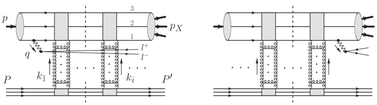
Figure 3: Total eikonalized amplitude of the diffractive Drell-Yan process, which effectively includes the gap survival effects.

Let us now write the total hadronic amplitude of the diffractive Drell-Yan process as KPST06

$$A_{if}=A^{(1)}_{if}+A^{(2)}_{if}+A^{(3)}_{if}\,,$$ (13)

where each term corresponds to $\gamma^{*}$ radiation by one of the valence quarks, in particular,

$$A^{(1)}_{if}(x_{\gamma 1},\vec{q}_{\perp},\lambda_{\gamma}) = \frac{i}{4}\,\alpha^{2}\int d^{2}r_{1}d^{2}r_{2}d^{2}r_{3}d^{2}rd^{2}bdx_{q_{1}}dx_{q_{2}}dx_{q_{3}}$$ (14)

$$\times \Psi_{i}(\vec{r}_{1},\vec{r}_{2},\vec{r}_{3};x_{q_{1}},x_{q_{2}},x_{q_{3}})\Psi_{f}^{*}(\vec{r}_{1}+\alpha\vec{r},\vec{r}_{2},\vec{r}_{3};x_{q_{1}}-x_{\gamma 1},x_{q_{2}},x_{q_{3}})$$

$$\times \Big{[}M^{\lambda_{\gamma}}_{\bar{q}q}(\vec{b},\vec{r}_{1}-\vec{r}_{2},\vec{r},\alpha)+M^{\lambda_{\gamma}}_{\bar{q}q}(\vec{b},\vec{r}_{1}-\vec{r}_{3},\vec{r},\alpha)\Big{]}e^{i\vec{l}_{\perp}\cdot\alpha\vec{r}}e^{i\vec{\delta}_{\perp}\cdot\vec{b}}$$

Here, $\lambda_{\gamma}=L,T$; $\vec{l}_{\perp}=\vec{\delta}_{\perp}-\vec{q}_{\perp}/\alpha$ ($z$-axis is directed along initial proton momentum); the hard photon with virtuality $q^{2}=M^{2}\gg m_{p}^{2}$, transverse $\vec{q}_{\perp}$ and fractional longitudinal $x_{\gamma 1}$ momenta is emitted from the first valence quark with impact parameter $\vec{r}_{1}$ (see Fig. 3), other two valence quarks in the proton have impact parameters $\vec{r}_{2}$ and $\vec{r}_{3}$, respectively; $\vec{r}$ is transverse separation between the photon and the radiating quark; $\alpha=x_{\gamma 1}/x_{q_{1}}$ is the fraction of longitudinal momenta taken away by the photon from the radiating quark; $M^{L,T}_{\bar{q}q}$ are the Fourier-transformed amplitudes for the elastic quark dipole scattering off the proton target accompanied by the hard $L,T$-polarized photon emission calculated above in Eq. (12); $\Psi_{i,f}$ are the light-cone wave functions of the $3q$ systems in the initial and final state, respectively. In Eq. (14) we implicitly assumed that exchanges $t$-channel gluons all together take a negligibly small longitudinal momentum compared to the collisions energy $\sqrt{s}$ and, hence, corrections to quark momenta due to gluon couplings are neglected in the wave functions.

Eikonalization of the universal elastic dipole-target scattering amplitude performed in Eq. (12) incorporates all soft and hard interactions between $\bar{q}q$ dipole and the target on the same footing as the parameterization for the amplitude on a free proton, $f_{el}(\vec{b},\vec{r})$, fitted to data on DIS and soft hadron scattering. This provides an alternative to the conventional treatment of the gap survival effects in terms of the single suppression factor in the cross section $\sigma_{DDY}=K\cdot\sigma_{DDY}^{bare}$, the so-called gap survival factor, estimated in the eikonal approximation KPS06

$$K=1-\frac{1}{\pi}\frac{\sigma_{tot}^{pp}(s)}{B_{sd}^{DY}(s)+2B_{el}^{pp}(s)}+\frac{1}{(4\pi)^{2}}\frac{[\sigma_{tot}^{pp}(s)]^{2}}{B_{el}^{pp}(s)[B_{sd}^{DY}(s)+B_{el}^{pp}(s)]}$$ (15)

where the energy-dependent elastic slope is $B_{el}^{pp}(s)=B_{el}^{0}+2\alpha_{{I\!\!P}}^{\prime}\ln(s/s_{0})$ with $B_{el}^{0}=7.5\,\textrm{GeV}^{-2},\,s_{0}=1\,\textrm{GeV}^{2}$. The slope of single-diffractive DY cross section can be estimated as, $B_{sd}^{DY}\simeq\langle r_{ch}^{2}\rangle/3+2\alpha_{{I\!\!P}}^{\prime}\ln(s/s_{0})$, where the proton mean charge radius squared $\langle r_{ch}^{2}\rangle=0.8$ fm². More elaborated models for the gap survival factor incorporating a part of the Gribov corrections (see e.g. Refs. gotsman ; kaidalov ) predict similar suppression factors, and one can easily replace the $K$-factor (15) by a preferable one.

In order to demonstrate that the eikonalization procedure (12) correctly takes into account soft gap survival effects, we checked that the ratio between diffractive Drell-Yan cross sections with eikonalized (12) and non-eikonalized (9) diffractive amplitude leads to a suppression factor which is very close numerically to the standard gap survival factor $K$ defined independently from Eq. (15),

$$\frac{\sigma_{DDY}^{eik}}{\sigma_{DDY}^{noneik}}\simeq K$$ (16)

and such a relation between them holds at different energies. And this ratio does not depend on $x_{\gamma 1}$ and $M^{2}$. This confirms our statement we have made in the beginning of this Section: the eikonalization of the elastic dipole-target amplitude correctly incorporates the unitarity corrections.

As was already been said above, the parameterizations for the real elastic dipole-target scattering fitted to experimental data must already effectively contain the absorptive and all-order QCD corrections, so it should not be eikonalized when used in explicit calculations, and no $K$-factors are to be applied to the cross section in this case.

Let us now shortly discuss different parameterizations for the elastic dipole-target scattering amplitude $f_{el}(\vec{b},\vec{r})$ corresponding to the scattering of small ($r\ll r_{p}$) and large ($r\sim r_{p}$) dipoles off the proton target, known from the data fits.

IV Elastic dipole-target scattering amplitude

It is well-known that small $x$ (large $Q^{2}$) regime corresponding to a scattering of small dipoles with $r\to 0$ is well described by the popular Golec-Biernat-Wuestoff (GBW) parametrization of the dipole cross section GBWdip . The elastic $b$-dependent amplitude in this case is $x$-dependent and has a form GBW-par (see also Ref. KST-GBW-eqs )

$$\mathrm{Im}f_{el}^{\rm{GBW}}(\vec{b},\vec{r},x,x_{q})=\frac{\sigma_{0}}{8\pi{\cal B}(x)}\Bigg{\{}\exp\Bigg{[}-\frac{[\vec{b}+\vec{r}(1-x_{q})]^{2}}{2{\cal B}(x)}\Bigg{]}+\exp\Bigg{[}-\frac{[\vec{b}+\vec{r}x_{q}]^{2}}{2{\cal B}(x)}\Bigg{]}$$

$$-\,2\exp\Bigg{[}-\frac{r^{2}}{R_{0}^{2}(x)}-\frac{[\vec{b}+\vec{r}(1/2-x_{q})]^{2}}{2{\cal B}(x)}\Bigg{]}\Bigg{\}},\qquad{\cal B}(x)=R_{N}^{2}(x)+R_{0}^{2}(x)/8\,,$$ (17)

where parameters are fitted to DIS data at small $x$ GBWdip $\sigma_{0}=23.03$ mb, $R_{0}(x)=0.4\,\mathrm{fm}\times(x/x_{0})^{0.144}$ with $x_{0}=3.04\times 10^{-4}$, $x\sim Q^{2}/s$ is the Bjorken variable, $x_{q}$ is the quark longitudinal quark fraction in the dipole defined in Eq. (27), $R_{N}^{2}(x)$ in the limit $r\to 0$ can be defined through the slope of elastic electroproduction of $\rho$-mesons measured at HERA as

$$R_{N}^{2}(x)=B_{\gamma^{*}p\to\rho p}(x,Q^{2}\gg 1\,\textrm{GeV}^{2})-R_{0}^{2}(x)/4,\quad B_{\gamma^{*}p\to\rho p}(x,Q^{2}\gg 1\textrm{GeV}^{2})\simeq 5\,\textrm{GeV}^{-2}$$

. Amplitude (17) correctly reproduces the dipole cross section GBWdip

$$2\int d^{2}b\,\mathrm{Im}f_{el}(\vec{r},\vec{b},x,x_{q})=\sigma_{\bar{q}q}(r,x)\,,$$

but contains more information, because it is sensitive to the color dipole orientation within the phenomenological saturation model, which includes contributions from higher order perturbative corrections as well as non-perturbative effects contained in DIS data.

Notice that the simple GBW parameterization (17) has some restrictions. In particular, the non-integrated gluon distribution exhibits no power-law tails in momentum space in contradiction with QCD. Moreover, it does not match the DGLAP evolution at large values of $Q^{2}$. Therefore, one should be cautious applying this model at very high transverse momenta accessible at the energies of LHC KST-GBW-eqs .

For soft scattering (moderate and small $Q^{2}$) corresponding to large dipoles $r\sim R_{0}(x)$, the c.m. energy squared $s$, rather than Bjorken $x$, is the proper variable. So, for the soft processes one can switch from $x$- to $s$-dependence KST99 , keeping the same functional form of the dipole amplitude (17) and adjusting the parameters to observables in soft reactions as kpss ; KST-par ; KST-GBW-eqs

$$\mathrm{Im}f^{\mathrm{GBW}}_{el}(\vec{b},\vec{r},x,x_{q})\quad \rightarrow \quad\mathrm{Im}f^{\mathrm{KST}}_{el}(\vec{b},\vec{r},s,x_{q}),$$ (18)

$$R_{0}(x)\quad \rightarrow \quad R_{0}(s)=0.88\,\mathrm{fm}\,(s_{0}/s)^{0.14},$$

$$R_{N}^{2}(x)\quad \rightarrow \quad R_{N}^{2}(s)=B_{el}^{\pi p}(s)-\frac{1}{4}R_{0}^{2}(s)-\frac{1}{3}\langle r_{ch}^{2}\rangle_{\pi},$$

$$\sigma_{0}\quad \rightarrow \quad\sigma_{0}(s)=\sigma_{tot}^{\pi p}(s)\Big{(}1+\frac{3R_{0}^{2}(s)}{8\langle r_{ch}^{2}\rangle_{\pi}}\Big{)},$$

where the pion-proton total cross section is parameterized as barnett $\sigma_{tot}^{\pi p}(s)=23.6(s/s_{0})^{0.08}$ mb, $s_{0}=1000\,\textrm{GeV}^{2}$, the mean pion radius squared is amendolia $\langle r_{ch}^{2}\rangle_{\pi}=0.44$ fm², and the Regge parametrization of the elastic slope $B_{el}^{\pi p}(s)=B_{0}+2\alpha^{\prime}_{{I\!\!P}}\ln(s/\mu^{2})$, with $B_{0}=6\,\textrm{GeV}^{-2}$, $\alpha^{\prime}_{{I\!\!P}}=0.25\,\textrm{GeV}^{-2}$, and $\mu^{2}=1\,\textrm{GeV}^{2}$ can be used. We shall refer to $\mathrm{Im}f^{\mathrm{KST}}_{\bar{q}q}(\vec{b},\vec{r},s,x_{q})$ below as the Kopeliovich-Schäfer-Tarasov (KST) parametrization of the elastic dipole-proton amplitude KST-par .

Two models for the elastic quark dipole-target scattering amplitude $f_{el}(\vec{b},\vec{r})$, given above by Eqs. (17) and (18), are valid for small $r\ll r_{p}$ and large $r\sim r_{p}$ dipole ($r_{p}$ is the mean proton size), respectively. Since the diffractive DY cross section is primarily sensitive to the large transverse separations $\sim r_{p}$ between target and projectile implied by the forward limit $t\to 0$, then the KST parameterization for the dipole cross section should be used, at least, in the leading order calculation. For completeness, we will compare the DDY cross sections calculated with GBW and KST parameterizations below when discussing the numerical results.

V Single diffractive Drell-Yan cross section

The differential cross section for the single diffractive di-lepton production in the target rest frame reads

$$d^{\,8}\sigma^{sd}_{\lambda_{\gamma}}(pp\to pl^{+}l^{-}X) = \sum_{f}\sum_{n=1}^{3}|A^{(n)}_{if}(x_{\gamma 1},\vec{q}_{\perp},\lambda_{\gamma})|^{2}\frac{d\alpha}{\alpha(1-\alpha)}\frac{d^{2}q_{\perp}d^{2}\delta_{\perp}}{(2\pi)^{5}\,8(p_{i,n}^{0})^{2}}$$ (19)

$$\times \alpha_{em}\epsilon_{\mu}(\lambda_{\gamma})\epsilon^{*}_{\nu}(\lambda_{\gamma})L^{\mu\nu}\frac{dM^{2}d\Omega}{16\pi^{2}M^{4}},\quad\lambda_{\gamma}=L,T$$

where prefactors provide averaging over colors and helicities of exchanged $t$-channel gluons, $p_{i,n}^{0}$ is the energy of the radiating $n$th quark in the initial state, $n=1,\,...,\,3$; $\alpha_{em}=e^{2}/(4\pi)=1/137$ is the electromagnetic coupling constant. The second line in Eq.(19) describes decay of $\gamma^{*}$ into the leptonic pair $l^{+}l^{-}$ into solid angle $d\Omega=d\phi d\cos\theta$, and the standard leptonic tensor is given by

$$L^{\mu\nu}=4(p_{l^{+}}^{\mu}p_{l^{-}}^{\nu}+p_{l^{+}}^{\nu}p_{l^{-}}^{\mu}-g^{\mu\nu}(p_{l^{+}}\cdot p_{l^{-}}))\,.$$

At the moment, we are not interested in lepton polarizations and their angular distributions, so for the sake of simplicity we integrate out the cross section (19) over the solid angle of the lepton pair. We keep in the cross section only diagonal in the photon polarization $\lambda_{\gamma}=L,T$ terms (non-diagonal ones drop out after integration over leptonic azimuthal angle $\phi$). Integrating the diffractive differential DY cross section over the photon transverse momentum $\vec{q}_{\perp}$ we get

$$\frac{d^{4}\sigma_{L,T}(pp\to pl^{+}l^{-}X)}{d\ln\alpha\,dM^{2}\,d^{2}\delta_{\perp}}=\frac{\alpha_{em}}{3\pi M^{2}}\,\frac{d^{3}\sigma_{L,T}(pp\to p\gamma^{*}X)}{d\ln\alpha\,d^{2}\delta_{\perp}}\,.$$ (20)

Then applying the completeness relation

$$\sum_{f}\Psi_{f}(\vec{r}_{1}+\alpha\vec{r},\vec{r}_{2},\vec{r}_{3};x_{q_{1}},x_{q_{2}},x_{q_{3}})\Psi^{*}_{f}(\vec{r}\,^{\prime}_{1}+\alpha\vec{r}\,^{\prime},\vec{r}\,^{\prime}_{2},\vec{r}\,^{\prime}_{3};x^{\prime}_{q_{1}},x^{\prime}_{q_{2}},x^{\prime}_{q_{3}})$$

$$\phantom{.......}=\,\delta(\vec{r}_{1}-\vec{r}\,^{\prime}_{1}+\alpha(\vec{r}-\vec{r}\,^{\prime}))\delta(\vec{r}_{2}-\vec{r}\,^{\prime}_{2})\delta(\vec{r}_{3}-\vec{r}\,^{\prime}_{3})\prod_{j=1}^{3}\delta(x_{q_{j}}-x^{\prime}_{q_{j}})$$ (21)

we get the diffractive $\gamma^{*}$ production cross section in the following differential form

$$\frac{d^{3}\sigma_{\lambda_{\gamma}}(pp\to p\gamma^{*}X)}{d\ln\alpha\,d^{2}\delta_{\perp}}=\frac{\sum_{q}Z_{q}^{2}}{64\pi^{2}}\int d^{2}r_{1}d^{2}r_{2}d^{2}r_{3}d^{2}r\,d^{2}bd^{2}b^{\prime}\,dx_{q_{1}}dx_{q_{2}}dx_{q_{3}}$$

$$\qquad\qquad\times\,|\tilde{\Psi}^{\lambda_{\gamma}}_{\gamma^{*}q}(\alpha,\vec{r})|^{2}|\Psi_{i}(\vec{r}_{1},\vec{r}_{2},\vec{r}_{3};x_{q_{1}},x_{q_{2}},x_{q_{3}})|^{2}$$

$$\qquad\qquad\times\,\Delta(\vec{r}_{1},\vec{r}_{2},\vec{r}_{3};\vec{b};\vec{r},\alpha)\Delta(\vec{r}_{1},\vec{r}_{2},\vec{r}_{3};\vec{b}\,^{\prime};\vec{r},\alpha)\,e^{i\vec{\delta}_{\perp}\cdot(\vec{b}-\vec{b}\,^{\prime})}$$ (22)

where $\tilde{\Psi}_{\gamma^{*}q}=\Psi_{\gamma^{*}q}/Z_{q}$, and

$$\Delta = -2\mathrm{Im}\,f^{\mathrm{KST}}_{el}(\vec{b},\vec{r}_{1}-\vec{r}_{2})+2\mathrm{Im}\,f^{\mathrm{KST}}_{el}(\vec{b},\vec{r}_{1}-\vec{r}_{2}+\alpha\vec{r})$$ (23)

$$-2\mathrm{Im}\,f^{\mathrm{KST}}_{el}(\vec{b},\vec{r}_{1}-\vec{r}_{3})+2\mathrm{Im}\,f^{\mathrm{KST}}_{el}(\vec{b},\vec{r}_{1}-\vec{r}_{3}+\alpha\vec{r})\,,$$

where the KST parameterization (18) fitted to the soft data and hence valid at $|\vec{r}_{i}-\vec{r}_{j}|\sim\vec{b},\,i\not=j$ is used. Finally, going over to the forward limit $\vec{\delta}_{\perp}=0$ we get

$$\frac{d^{3}\sigma_{\lambda_{\gamma}}(pp\to p\gamma^{*}X)}{d\ln\alpha\,d\delta_{\perp}^{2}}\Big{|}_{\delta_{\perp}=0}=\frac{\sum_{q}Z_{q}^{2}}{64\pi}\int d^{2}r_{1}d^{2}r_{2}d^{2}r_{3}d^{2}r\,dx_{q_{1}}dx_{q_{2}}dx_{q_{3}}$$

$$\qquad\times\,|\tilde{\Psi}^{\lambda_{\gamma}}_{\gamma^{*}q}(\alpha,\vec{r})|^{2}|\Psi_{i}(\vec{r}_{1},\vec{r}_{2},\vec{r}_{3};x_{q_{1}},x_{q_{2}},x_{q_{3}})|^{2}\,\left[\int d^{2}b\,\Delta(\vec{r}_{1},\vec{r}_{2},\vec{r}_{3};\vec{b};\vec{r},\alpha)\right]^{2}$$ (24)

We see that normalization of the cross section agrees with the original result of Ref. KPST06 . The total diffractive cross section is then given by

$$\frac{d\sigma(pp\to p\gamma^{*}X)}{d\ln\alpha}=\frac{1}{B_{sd}^{DY}(s)}\frac{d^{3}\sigma(pp\to p\gamma^{*}X)}{d\ln\alpha\,d\delta_{\perp}^{2}}\Big{|}_{\delta_{\perp}=0}$$ (25)

where $B_{sd}^{DY}(s)$ is the diffractive slope similar to the one measured in diffractive DIS.

The next step is to introduce the proton wave function assuming the Gaussian shape for the quark distributions in the proton as

$$|\Psi_{i}(\vec{r}_{1},\vec{r}_{2},\vec{r}_{3};x_{q_{1}},x_{q_{2}},x_{q_{3}})|^{2} = \frac{2+a/b}{\pi^{2}ab}\exp\Big{[}-\frac{r_{1}^{2}}{a}-\frac{r_{2}^{2}+r_{3}^{2}}{b}\Big{]}\rho(x_{q_{1}},x_{q_{2}},x_{q_{3}})$$ (26)

$$\times \delta(\vec{r}_{1}+\vec{r}_{2}+\vec{r}_{3})\delta(1-x_{q_{1}}-x_{q_{2}}-x_{q_{3}})$$

where $a=\langle r_{\bar{q}q}^{2}\rangle$ and $b=\langle R_{q}^{2}\rangle$ are the diquark mean radius squared and the quark mean distance from the diquark squared, respectively. In this work, we will use the simplest case of symmetric valence quarks distribution assuming that $r_{\bar{q}q}=R_{q}=0.85$ fm.

Then valence quark distribution in the proton is given by

$$\int dx_{q_{2}}dx_{q_{3}}\rho(x_{q_{1}},x_{q_{2}},x_{q_{3}})=\rho_{q_{1}}(x_{q_{1}})\,.$$

where we integrated out the longitudinal fractions of the diquark in the proton. Generalization of the three-body proton wave function (26) including different quark and antiquark flavors leads to the proton structure function KRT00

$$\sum_{q}Z_{q}^{2}[\rho_{q}(x_{q})+\rho_{\bar{q}}(x_{q})]=\frac{1}{x_{q}}F_{2}(x_{q}),\qquad x_{q}=\frac{x_{\gamma 1}}{\alpha}\,.$$ (27)

In the numerical analysis below, in order to estimate the theoretical uncertainty in the diffractive DY process we will use a few different parameterizations for the proton structure function $F_{2}$, widely used in the literature.

VI Numerical results

Let us now turn to discussion of the numerical results. We start from the comparison of the differential cross sections for single diffractive and inclusive Drell-Yan processes. In Fig. 4 the ratio of the diffractive to inclusive DY cross sections is plotted as a function of di-lepton invariant mass squared $M^{2}$ (left panel) and photon fractional light-cone momentum $x_{\gamma 1}$ (right panel) at different energies. In the left panel, the curves are given for fixed $x_{\gamma 1}=0.5$ (solid lines) and $x_{\gamma 1}=0.9$ (dashed lines). In the right panel, the curves are given for fixed $M^{2}=50\,\textrm{GeV}^{2}$ (solid lines) and $M^{2}=500\,\textrm{GeV}^{2}$ for $\sqrt{s}=14$ TeV and 500 GeV, and $M^{2}=200\,\textrm{GeV}^{2}$ at $\sqrt{s}=40$ GeV (dashed lines). The pairs of solid/dashed curves in the both panels correspond to $\sqrt{s}=40\,\textrm{GeV}$, $500$ GeV and $14$ TeV from top to bottom, respectively. Here we used the KST parameterization for the dipole-target scattering amplitude kpss ; KST-GBW-eqs ; KST-par and $F_{2}$ parameterization by Cudell and Soyez Cudell-F2 are used here and below unless otherwise is specified. Unitarity corrections are included by default into the employed phenomenological partial elastic dipole amplitude fitted to data (see above). In this calculation we consider the unpolarized case summing up the contributions of longitudinal and transverse parts both in the diffractive and inclusive cross sections.

Figure 4: The ratio of the diffractive to inclusive Drell-Yan cross sections as function of the lepton-pair invariant mass squared $M^{2}$ (left panel) and photon fraction $x_{\gamma 1}$ (right panel) at different energies. In the left panel, the curves are given for fixed $x_{\gamma 1}=0.5$ (solid lines) and $x_{\gamma 1}=0.9$ (dashed lines). In the right panel, the curves are given for fixed $M^{2}=50\,\textrm{GeV}^{2}$ (solid lines) and $M^{2}=500\,\textrm{GeV}^{2}$ for $\sqrt{s}=14$ TeV and 500 GeV, and $M^{2}=200\,\textrm{GeV}^{2}$ at $\sqrt{s}=40$ GeV (dashed lines). The pairs of solid/dashed curves in the both panels correspond to $\sqrt{s}=40\,\textrm{GeV}$, $500$ GeV and $14$ TeV from top to bottom, respectively.

As seen from Fig. 4, the DDY-to-DY cross section ratio is falling with energy. However, naively one could expect basing on QCD factorisation, that the DDY cross section, which is proportional to the dipole cross section squared, should rise with energy steeper than the total inclusive cross section. At the same time, the ratio rises with the hard scale of the process, $M^{2}$. This also looks counterintuitive, since diffraction is usually associated with soft interactions deriv1 . These effects are different from ones emerging in Regge factorisation-based calculations, where we observe a slow rise of the DDY-to-DY cross section ratio with c.m.s. energy and its practical independence on the hard scale of the process $M^{2}$ Antoni11 .

In order to understand such an interesting shape of the energy and hard scale dependence of the DDY-to-DY cross section ratio obtained in the color dipole approach, let us look at the amplitude of the DDY process, which is proportional to the difference between the dipole cross sections of the Fock states with and without the hard photon emission KPST06 , i.e.

$$M_{DDY}\sim\sigma(\vec{R})-\sigma(\vec{R}-\alpha\vec{r})=\frac{2\alpha\sigma_{0}}{R_{0}^{2}(x)}e^{R^{2}/R_{0}^{2}(x)}\,\left(\vec{r}\cdot\vec{R}\right)+h.o.$$ (28)

assuming the simplest GBW slope for the dipole cross section, and the hardness of the emitted photon implies $r\sim 1/M\ll R_{0}(x)$. We see now that the diffractive DY amplitude is linear in $r$, so the diffractive cross section turns out to be a quadratic function of $r$, which is different from e.g. the diffractive DIS process where the cross section is proportional to $r^{4}$ and is dominated by soft fluctuations (see e.g. Refs. KPSdiff ; BP97 ). Since the diffractive DY cross section is proportional to $r^{2}$, then soft and hard interactions contribute on the same footing KPST06 , which is one of the basic sources of the QCD factorisation breaking in diffractive DY process.

As was demonstrated in Ref. KPST06 , all the energy and scale dependence of the DDY-to-DY cross section ratio comes via the $x$-dependent factor,

$$\frac{\sigma_{DDY}}{\sigma_{DY}}\propto\frac{1}{R_{0}^{2}(x)}e^{-2R^{2}/R_{0}^{2}(x)}$$ (29)

where $x=M^{2}/x_{\gamma 1}s$. In our case, $R_{0}^{2}(x)<2R^{2}$, so the factor in Eq. (29) rises with $R_{0}(x)$, i.e. with $x$. This is the main reason why the ratio shown in Fig. 4 decreases with energy, but increases with the hard scale $M^{2}$. Also, the falling energy behavior is partly due to the rise with energy of the absorptive corrections KPST06 .

Figure 5: The ratio of the longitudinal (L) to transverse (T) photon polarization contributions to the diffractive Drell-Yan cross section as function of the lepton-pair invariant mass squared $M^{2}$ (left panel) and photon fraction $x_{\gamma 1}$ (right panel) at different energies: $\sqrt{s}=40$ GeV (dash-dotted lines), $\sqrt{s}=500$ GeV (solid lines) and $\sqrt{s}=14$ TeV (dashed lines). In the left panel, the curves are given for fixed $x_{\gamma 1}=0.5$ (upper three curves) and $x_{\gamma 1}=0.9$ (lower three curves). In the right panel, the curves are given for fixed $M^{2}=50\,\textrm{GeV}^{2}$.

In Fig. 5 we show the relative contribution of the longitudinal (L) to transverse (T) photon polarization to the diffractive Drell-Yan cross section. The ratio $\sigma_{L}/\sigma_{T}$ is presented as function of lepton-pair invariant mass squared $M^{2}$ (left panel) and photon fraction $x_{\gamma 1}$ (right panel) at different energies: $\sqrt{s}=40$ GeV (dash-dotted lines), $\sqrt{s}=500$ GeV (solid lines) and $\sqrt{s}=14$ TeV (dashed lines). In the left panel, the curves are given for fixed $x_{\gamma 1}=0.5$ (upper three curves) and $x_{\gamma 1}=0.9$ (lower three curves). In the right panel, the curves are given for fixed $M^{2}=50\,\textrm{GeV}^{2}$. We see that the diffractive DY process is always dominated by radiation of transversely polarized lepton pairs. The ratio $\sigma_{L}/\sigma_{T}$ is only slightly dependent on $M^{2}$, and there is no any significant energy dependence. The longitudinal photon polarization amounts to about 10 % at $x_{\gamma 1}=0.5$ and then steeply falls down at large $x_{\gamma 1}\to 1$. Such a behavior turns out to be similar to that for inclusive DY process KPST06 .

Figure 6: Diffractive Drell-Yan cross section (in fb) as function of the lepton-pair invariant mass squared $M^{2}$ (left panel) and photon fraction $x_{\gamma 1}$ (right panel) at the RHIC II c.m.s. energy $\sqrt{s}=500$ GeV. In the left panel, the curves are given for fixed $x_{\gamma 1}=0.5$ with GBW (long-dashed line) and KST (solid line) parameterizations, and for $x_{\gamma 1}=0.9$ with GBW (dash-dotted line) and KST (dashed line) parameterizations. In the right panel, the curves are given for fixed $M^{2}=50\,\textrm{GeV}^{2}$ with GBW (long-dashed line) and KST (solid line) parameterizations, and for $M^{2}=500\,\textrm{GeV}^{2}$ with GBW (dash-dotted line) and KST (dashed line) parameterizations.

We also compare predictions for the diffractive DY cross section for different parameterizations for elastic dipole-target scattering amplitude corresponding to scattering of small (GBW given by Eq. (17)) and large (KST given by Eq. (18)) dipoles. As an example, in Fig. 6 we present the diffractive Drell-Yan cross section as function of the lepton-pair invariant mass squared $M^{2}$ (left panel) and photon fraction $x_{\gamma 1}$ (right panel) at the RHIC II c.m.s. energy $\sqrt{s}=500$ GeV. We notice that the GBW parameterization leads to roughly a factor of two smaller cross section than the one obtained with the KST parameterization, however, both of them exhibit basically the same $x_{\gamma 1}$ and $M^{2}$ shapes. It means that the evolution of the dipole size can only affect the overall normalization of the DDY cross section. Since arguments in the elastic amplitude $f_{el}$ in Eq. (12), the impact distance between the target and the projectile $b$ and the transverse distance between projectile quarks $r_{p}\sim|\vec{r}_{i}-\vec{r}_{j}|,\,i\not=j$, are of the same order and given at the soft hadronic scale, then the use of KST parameterization fitted to the soft hadron scattering data data is justified in the case of diffractive DY.

Figure 7: Diffractive Drell-Yan cross section (in fb) as function of the lepton-pair invariant mass squared $M^{2}$ (left panel) with fixed $x_{\gamma 1}=0.5$ and photon fraction $x_{\gamma 1}$ with fixed $M^{2}=50\,\textrm{GeV}^{2}$ (right panel) for different parameterizations of the proton structure function $F_{2}$: Regge parameterization by Cudell et al Cudell-F2 (solid line), SMC parameterization SMC with infrared freezing at two different scales $Q_{0}^{2}=0.1$ (dashed line) and 0.5 $\textrm{GeV}^{2}$ (long-dashed line) and GJR parameterization GJR (dash-dotted line).

In order to illustrate the intrinsic theoretical uncertainties in our DDY cross section calculations, in Fig. 7 we show the diffractive DY cross section as function of the lepton-pair invariant mass squared $M^{2}$ (left panel) and photon fraction $x_{\gamma 1}$ (right panel) for different parameterizations of the proton structure function $F_{2}$ entering the DDY cross section through Eq. (27). In this figure we represent results with four distinct cases widely used in the literature: Regge parameterization by Cudell and Soyez Cudell-F2 (solid line), old SMC parameterization SMC with infrared freezing at two different scales $Q_{0}^{2}=0.1$ (dashed line) and 0.5 $\textrm{GeV}^{2}$ (long-dashed line) and recent GJR parameterization GJR (dash-dotted line). We see that the diffractive DY cross section is sensitive to various $F_{2}$ parameterizations, especially at relatively large $x_{\gamma 1}\to 1$, which is reflected in quite noticeable uncertainties in our calculation. This opens up a promising opportunity to use the diffractive DY reaction as a direct probe of the proton structure function at rather large $x=x_{\gamma 1}/\alpha$.

The Regge parameterization Cudell-F2 is presumably constructed in the soft region where the most of the contribution to the DDY process comes from, and it leads to a rather regular and stable behavior of the cross section at $x_{\gamma 1}\to 1$. Old SMC $F_{2}$ parameterization is obviously inapplicable to the DDY calculations, because it leads to significant uncertainties with respect to the lower freezing scale $Q_{0}$ variations indicating at a strong sensitivity to the non-perturbative low-$Q$ region where the proton structure function $F_{2}$ is unknown to a large extent.

VII Conclusion and outlook

In this work, we have investigated in detail the QCD factorisation breaking effects in the diffractive Drell-Yan process within the framework of the color dipole approach. Such effects lead to quite different properties of the corresponding observables with respect to QCD factorisation-based calculations.

A quark cannot diffractively radiate a photon in the forward direction, whereas a hadron can due to the presence of transverse motion of spectator quarks in the projectile hadron. For this reason, the diffractive DY cross section depends on the hadronic size breaking the QCD factorisation.

This leads to the physical picture where hard and soft interactions are equally important for DY diffraction, and their relative contributions are independent of the hard scale, like in the inclusive DY process. This is a result of the specific property of DY diffraction: its cross section is a linear, rather than quadratic function of the dipole cross section. On the contrary, diffractive DIS is predominantly a soft process, because its cross section is proportional to the dipole cross section squared.

Contrary to what follows from the calculations based on QCD factorisation, the ratio of the diffractive to inclusive cross sections falls with energy, but rises with the di-lepton effective mass $M$. This happens due to the saturated behavior of the dipole cross section which levels off at large separations. All these properties are different from those in the diffractive DIS process, where QCD factorisation is exact.

In addition, we made predictions for the differential (in photon fractional momentum $x_{\gamma 1}$ and di-lepton invariant mass squared $M^{2}$) cross sections for the diffractive DY process at the energies of RHIC (500 GeV) and LHC (14 TeV). The transverse photon polarisation gives the dominant contribution to the DDY cross section. The ratio $\sigma_{L}/\sigma_{T}$ is almost independent on c.m.s. energy $\sqrt{s}$ and only weakly depends on the hard scale $M^{2}$.

Finally, we propose an alternative treatment of the absorptive effects describing the subsequent soft interactions of projectile quarks off the proton target by multiple elastic dipole-target scatterings. Such an idea leads to eikonalization of the “bare” elastic dipole amplitude in the DDY amplitude and, ultimately, to a description of the gap survival effects on the same footing with the leading-order diffractive DY subprocess in the framework of the color dipole approach without introducing the gap survival factor $K$. These corrections are included by default into the employed phenomenological partial elastic dipole amplitude fitted to data.

The main features of the diffractive Drell-Yan reaction described above are valid for other diffractive Abelian processes, like production of direct photons, Higgsstrahlung, radiation of $Z$ and $W$ bosons. A detailed analysis of these processes in the framework of the color dipole approach is planned for a forthcoming study.

Acknowledgments

Useful discussions and helpful correspondence with Jochen Bartels, Antoni Szczurek, Gunnar Ingelman and Mark Strikman are gratefully acknowledged. This study was partially supported by the Carl Trygger Foundation (Sweden), by Fondecyt (Chile) grant 1090291, and by Conicyt-DFG grant No. 084-2009. Authors are also indebted to the Galileo Galilei Institute of Theoretical Physics (Florence, Italy) and to the INFN for partial support and warm hospitality during completion of this work.

References

- (1) R. J. Glauber, Phys. Rev. 100, 242 (1955).
- (2) E. Feinberg and I. Ya. Pomeranchuk, Nuovo. Cimento. Suppl. 3 (1956) 652.
- (3) M. L. Good and W. D. Walker, Phys. Rev. 120 (1960) 1857.
- (4) B. Z. Kopeliovich, I. K. Potashnikova, I. Schmidt, Braz. J. Phys. 37, 473-483 (2007). [arXiv:hep-ph/0604097 [hep-ph]].
- (5) B. Z. Kopeliovich, I. K. Potashnikova, I. Schmidt, A. V. Tarasov, Phys. Rev. D74, 114024 (2006) [hep-ph/0605157].
- (6) R. Pasechnik, to appear in Proceedings of the International Workshop “Low-x Meeting”, June 3-7, 2011
- (7) G. Kubasiak, A. Szczurek, Phys. Rev. D84, 014005 (2011). [arXiv:1103.6230 [hep-ph]].
- (8) A. Donnachie, P. V. Landshoff, Nucl. Phys. B303, 634 (1988).
- (9) G. Ingelman, P. E. Schlein, Phys. Lett. B152 256 (1985).
- (10) K. Wijesooriya, P. E. Reimer and R. J. Holt, Phys. Rev. C72, 065203 (2005).
- (11) B. Z. Kopeliovich, L. I. Lapidus, A. B. Zamolodchikov, JETP Lett. 33, 595-597 (1981).
- (12) G. Bertsch, S. J. Brodsky, A. S. Goldhaber, J. F. Gunion, Phys. Rev. Lett. 47, 297 (1981).
- (13) B. Z. Kopeliovich, proc. of the workshop Hirschegg 95: Dynamical Properties of Hadrons in Nuclear Matter, Hirschegg January 16-21, 1995, ed. by H. Feldmeyer and W. Nörenberg, Darmstadt, 1995, p. 102 (hep-ph/9609385);
- (14) S. J. Brodsky, A. Hebecker, and E. Quack, Phys. Rev. D55 (1997) 2584.
- (15) B. Z. Kopeliovich and B. Povh, Z. Phys. A356, 467 (1997).
- (16) R. Pasechnik, R. Enberg, G. Ingelman, Phys. Lett. B695, 189-193 (2011) [arXiv:1004.2912 [hep-ph]]; Phys. Rev. D82, 054036 (2010) [arXiv:1005.3399 [hep-ph]].
- (17) B. Z. Kopeliovich, I. K. Potashnikova, I. Schmidt, M. Siddikov, Phys. Rev. C84, 024608 (2011) [arXiv:1105.1711 [hep-ph]].
- (18) J. Bartels, S. Bondarenko, K. Kutak and L. Motyka, Phys. Rev. D73, 093004 (2006).
- (19) M. G. Ryskin, A. D. Martin, V. A. Khoze, Eur. Phys. J. C60, 265-272 (2009) [arXiv:0812.2413 [hep-ph]].
- (20) B. Z. Kopeliovich, A. Schäfer, A. V. Tarasov, Phys. Rev. D62, 054022 (2000). [arXiv:hep-ph/9908245 [hep-ph]].
- (21) L. D. Landau, I. Ya. Pomeranchuk, ZhETF, 505 (1953); Doklady AN SSSR 92, 535, 735 (1953).
- (22) B. Z. Kopeliovich, I. K. Potashnikova, I. Schmidt, A. V. Tarasov, Phys. Rev. D76, 034019 (2007) [hep-ph/0702106].
- (23) A. Donnachie, P. V. Landshoff, Nucl. Phys. B303, 634 (1988).
- (24) J. C. Collins, L. Frankfurt, M. Strikman, Phys. Lett. B307, 161-168 (1993) [hep-ph/9212212].
- (25) J. C. Collins, Phys. Rev. D57, 3051-3056 (1998) [hep-ph/9709499].
- (26) J. Raufeisen, J. C. Peng and G. C. Nayak, Phys. Rev. D66, 034024 (2002).
- (27) B. Z. Kopeliovich, A. Schaefer and A. V. Tarasov, Phys. Rev. C59, 1609 (1999), extended version in hep-ph/9808378.
- (28) M. S. Dubovikov, B. Z. Kopeliovich, L. I. Lapidus and K. A. Ter-Martirosian, Nucl. Phys. B 123 (1977) 147.
- (29) S. J. Brodsky and P. Hoyer, Phys. Lett. B 298 (1993) 165 [arXiv:hep-ph/9210262].
- (30) B. Z. Kopeliovich, I. K. Potashnikova, I. Schmidt, Phys. Rev. C73, 034901 (2006). [hep-ph/0508277].
- (31) E. Gotsman, E. M. Levin, and U. Maor, Z. Phys. C57, 677 (1993); Phys. Rev. D49, 4321 (1994); Phys. Lett. B353, 526 (1995); Phys. Lett. B347, 424 (1995).
- (32) A. B. Kaidalov, V. A. Khoze, A. D. Martin, and M. G. Ryskin, Eur. Phys. J. C33, 261 (2004).
- (33) K. J. Golec-Biernat, M. Wusthoff, Phys. Rev. D59, 014017 (1998). [hep-ph/9807513].
- (34) B. Z. Kopeliovich, H. J. Pirner, A. H. Rezaeian and I. Schmidt, Phys. Rev. D77, 034011 (2008) [arXiv:0711.3010 [hep-ph]].
- (35) B. Z. Kopeliovich, A. H. Rezaeian, I. Schmidt, Phys. Rev. D78, 114009 (2008) [arXiv:0809.4327 [hep-ph]].
- (36) B. Z. Kopeliovich, I. K. Potashnikova, I. Schmidt and J. Soffer, Phys. Rev. D 78, 014031 (2008) [arXiv:0805.4534 [hep-ph]].
-
(37)
B. Z. Kopeliovich, A. Schäfer and A. V. Tarasov, Phys. Rev. D62, 054022 (2000) [arXiv:hep-ph/9908245];
B. Z. Kopeliovich, I. K. Potashnikova, I. Schmidt, J. Soffer, Phys. Rev. D78, 014031 (2008) [arXiv:0805.4534 [hep-ph]]. - (38) R M. Barnett et al., Rev. Mod. Phys. 68, 611 (1996).
- (39) S. Amendolia et al., Nucl. Phys. B277, 186 (1986).
- (40) B. Z. Kopeliovich, J. Raufeisen, A. V. Tarasov, Phys. Lett. B503, 91-98 (2001). [hep-ph/0012035].
- (41) J. R. Cudell, G. Soyez, Phys. Lett. B516, 77-84 (2001). [hep-ph/0106307].
- (42) SMC Collaboration, B. Adeva et al, Phys. Rev. D58, 112001 (1998).
- (43) M. Gluck, P. Jimenez-Delgado and E. Reya, Eur. Phys. J. C 53, 355 (2008) [arXiv:0709.0614 [hep-ph]].