On the efficient representation of the half-space impedance Green’s function for the Helmholtz equation

Abstract

A classical problem in acoustic (and electromagnetic) scattering concerns the evaluation of the Green’s function for the Helmholtz equation subject to impedance boundary conditions on a half-space. The two principal approaches used for representing this Green’s function are the Sommerfeld integral and the (closely related) method of complex images. The former is extremely efficient when the source is at some distance from the half-space boundary, but involves an unwieldy range of integration as the source gets closer and closer. Complex image-based methods, on the other hand, can be quite efficient when the source is close to the boundary, but they do not easily permit the use of the superposition principle since the selection of complex image locations depends on both the source and the target. We have developed a new, hybrid representation which uses a finite number of real images (dependent only on the source location) coupled with a rapidly converging Sommerfeld-like integral. While our method applies in both two and three dimensions, we restrict the detailed analysis and numerical experiments here to the two-dimensional case.
Keywords: Helmholtz, impedance, Green’s function, layered media, Robin boundary conditions, Sommerfeld integral, complex images, half-space

1 Introduction

A number of problems in acoustics (and electromagnetics) involve the solution of the Helmholtz equation,

$$(\triangle+k^{2})u(\boldsymbol{x})=f(\boldsymbol{x})\,,$$ (1.1)

in the half-space $P=\{(x,y)\in{\mathbb{R}}^{2}:y>0\}$ or $S=\{(x,y,z)\in{\mathbb{R}}^{3}:z>0\}$, subject to suitable boundary and radiation conditions. In acoustics, the Helmholtz coefficient $k$ is given by $k=\frac{\omega}{c}$, where $\omega$ is the governing angular frequency (assuming a time-harmonic motion dependency of $e^{-i\omega t}$) and $c$ is the sound speed. In the present paper, we assume $k\in\mathbb{C}$ is constant throughout the region of interest, with ${\rm Re}(k)\geq 0$ and ${\rm Im}(k)\geq 0$. For concreteness, we concentrate initially on the two-dimensional problem of computing the scattered field due to a unit-strength point source located at $\boldsymbol{x}_{0}=(x_{0},y_{0})$ in the presence of a ”sound-hard” obstacle over an infinite half-space subject to impedance boundary conditions (Figure 1).

We let the total field be defined as $u^{tot}=u^{in}+u$, where $u^{in}$ denotes the (known) incoming field due to the point source and $u$ denotes the scattered field. On a sound-hard obstacle $\Omega$ with boundary $\Gamma$, the total field must satisfy homogeneous Neumann boundary conditions. Since the scattered field involves no sources outside $\Omega$, it must satisfy the homogeneous Helmholtz equation

$$(\triangle+k^{2})u(\boldsymbol{x})=0\$$ (1.2)

for $\boldsymbol{x}\in P\setminus\Omega$ . On the obstacle boundary $\Gamma$, we have

$$\frac{\partial u}{\partial n}=-\frac{\partial u^{in}}{\partial n},$$ (1.3)

where $\frac{\partial}{\partial n}$ is the outward normal derivative. Finally, on the interface, we assume a standard impedance condition on the total field of the form:

$$\frac{\partial u^{tot}}{\partial n}-i\alpha u^{tot}=0.$$ (1.4)

Since the interface is the $x$-axis, we have $\frac{\partial}{\partial n}=-\frac{\partial}{\partial y}$. In physically-motivated problems, an impedance condition is typically used to approximate a more complicated wave/surface interaction, such as scattering from a rough surface, an underlying porous medium, a complicated surface coating, etc. (see [2, 7]). In many applications, $\alpha=\beta k$, with $0\leq\beta\leq 1$, in which case any dissipation is due entirely to the imaginary part of $k$. The parameter $\beta$ in this context is called the surface admittance. In other cases, the physical model introduces dissipation of some other kind, resulting in a complex valued $\alpha$, even when $k$ is real. For the purposes of this paper, we will assume that $\alpha\in\mathbb{C}$, with ${\rm Re}(\alpha)\geq 0$, ${\rm Im}(\alpha)\geq 0$, $|\alpha|\leq|k|$, and leave aside any further discussion of the modeling. The Green’s function analysis of the present paper can be generalized to other values of $\alpha$, but we restrict our attention to $\alpha$ in the indicated range for the sake of simplicity. A second simplification is that we only consider the case of constant $\alpha$ (i.e. we do not permit $\alpha$ to vary along the length of the half-space interface). There is a substantial literature on impedance problems and we mention only a few relevant papers which also discuss the computation of the corresponding Green’s function. These include [5, 6, 11, 8, 14, 26, 30, 32, 33].

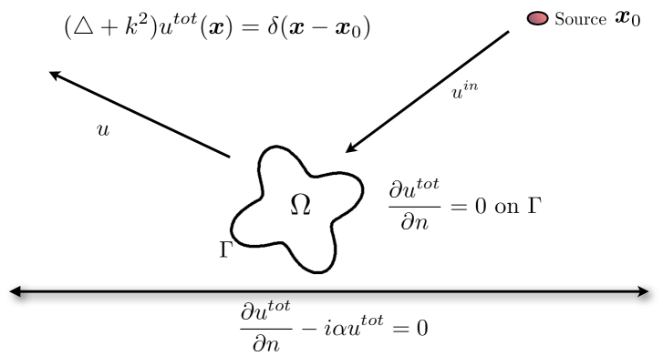
Figure 1: Scattering from a sound-hard obstacle above an impedance plane.

Returning now to the scattering problem (1.2, 1.3, 1.4), an ansatz for the solution is to represent the total field as

$$u^{tot}(\boldsymbol{x})=\int_{\Gamma}g_{k,\alpha}(\boldsymbol{x},\boldsymbol{y})\,\sigma(\boldsymbol{y})\,d{\boldsymbol{y}(s)}+u^{in}(\boldsymbol{x}),$$ (1.5)

where $s$ is arclength along $\Gamma$, $g_{k,\alpha}(\boldsymbol{x},\boldsymbol{x}_{0})$ is the Green’s function for the half-space $P$ with homogeneous impedance boundary conditions, and $u^{in}(\boldsymbol{x})=g_{k,\alpha}(\boldsymbol{x},\boldsymbol{x}_{0})$. Imposing the Neumann conditions (1.3) on $\Gamma$ yields the Fredholm integral equation of the second kind:

$$-\frac{1}{2}\sigma(\boldsymbol{x})+\int_{\Gamma}\frac{\partial}{\partial n_{x}}g_{k,\alpha}(\boldsymbol{x},\boldsymbol{y})\,\sigma(\boldsymbol{y})\,d{\boldsymbol{y}(s)}=-\frac{\partial}{\partial n_{x}}g_{k,\alpha}(\boldsymbol{x},\boldsymbol{x}_{0})$$ (1.6)

for $\boldsymbol{x}\in\Gamma$, where the integral is interpreted in the principal value sense. Equation (1.6) is invertible except for a countable sequence of spurious resonances $\{k_{j}\}$. Resonance-free, but more complicated, representations are well-known [11], which we will not review here, since we are primarily interest in the question of how to efficiently evaluate the impedance Green’s function $g_{k,\alpha}$ itself. In our examples, we will always assume $k\notin\{k_{j}\}$ and that equation (1.6) is solvable. Note that, by using the impedance Green’s function in the integral representation, the infinite half-space boundary does not need to be discretized.

Algorithms for the computation of $g_{k,\alpha}$ date back to the classical work of Sommerfeld, Weyl, and Van der Pol [31, 34, 33], who developed both what are now referred to as the Sommerfeld integral and the method of complex images. For more recent treatments of this problem, see [19, 12, 13, 26, 32, 24].

The main contribution of the present work is the observation that a finite number of real images can accurately capture the high-frequency components of the Sommerfeld integral. This leads, naturally, to a hybrid representation of the Green’s function in terms of a rapidly converging Sommerfeld-type representation, augmented with $\mathcal{O}(\log(1/d))$ real images for each source point that lies a distance $d$ from the impedance interface. Our approach is somewhat related to that of Cai and Yu [5], which also separates low- and high-frequency contributions, but uses an asymptotic method for the high-frequency components.

The paper is organized as follows. Section 2 gives a derivation of the classical spectral representation for the free space Green’s function, due to Sommerfeld. In Section 3, we discuss Sommerfeld and Van der Pol’s extension of the spectral representation to the case of impedance boundary conditions for a half-space. Section 4 introduces analytical (closed-form) expressions for the real and complex image representations. In Section 5, we present our new representation that combines a finite segment of real images in the lower half-space with a Sommerfeld integral that is rapidly decaying. Section 6 discusses some the details concerning discretization and quadrature for both the image segment and the obstacle boundary $\Gamma$, and Section 7 contains several numerical experiments which demonstrate the effectiveness of the scheme. Lastly, in Section 8, we discuss the extension of the method to the three-dimensional case, to layered media, and to the Maxwell equations - all areas for future research.

2 Spectral representation of the Green’s function

The solution $g_{k}$ to the Helmholtz equation

$$(\triangle+k^{2})g_{k}(\boldsymbol{x})=\delta(\boldsymbol{x}-\boldsymbol{x}_{0}),$$ (2.1)

in an infinite homogeneous medium is referred to as the free-space Green’s function, where $\boldsymbol{x}=(x,y)\in\mathbb{R}^{d}$, $d$ is the underlying dimension, and $\delta(\boldsymbol{x}-\boldsymbol{x}_{0})$ represents the Dirac delta function centered at $\boldsymbol{x}_{0}$. It is well known that

$$g_{k}(\boldsymbol{x},\boldsymbol{x}_{0})=\left\{\begin{array}[]{cc}\frac{i}{4}H^{(1)}_{0}(k|\boldsymbol{x}-\boldsymbol{x}_{0}|)&{\rm for}\ d=2,\\ &\\ -{\frac{e^{ik|\boldsymbol{x}-\boldsymbol{x}_{0}|}}{4\pi|\boldsymbol{x}-\boldsymbol{x}_{0}|}}&{\rm for}\ d=3,\end{array}\right.$$

where $H^{(1)}_{0}$ denotes the zeroth-order Hankel function of the first kind. These Green’s functions satisfy the outgoing Sommerfeld radiation condition

$$\lim_{r\to\infty}r^{(d-1)/2}\left(\frac{\partial}{\partial r}g_{k}(\boldsymbol{x},\boldsymbol{x}_{0})-ik\,g_{k}(\boldsymbol{x},\boldsymbol{x}_{0})\right),$$ (2.2)

where $r=|\boldsymbol{x}-\boldsymbol{x}_{0}|$.

A continuous spectral representation of the Green’s functions can be obtained by taking the Fourier transform of equation (2.1). In two dimensions, the Green’s function can then be written as

$$g_{k}(\boldsymbol{x},\boldsymbol{x}_{0})=\frac{1}{4\pi^{2}}\int_{-\infty}^{\infty}\int_{-\infty}^{\infty}\frac{e^{i(\lambda_{x}(x-x_{0})+\lambda_{y}(y-y_{0}))}}{\lambda_{x}^{2}+\lambda_{y}^{2}-k^{2}}\,d\lambda_{x}\,d\lambda_{y}.$$ (2.3)

Evaluating the integral in $\lambda_{y}$ via contour deformation yields the expansion in plane waves (often called the Sommerfeld integral):

$$g_{k}(\boldsymbol{x},\boldsymbol{x}_{0})=\frac{1}{4\pi}\int_{-\infty}^{\infty}\frac{e^{-\sqrt{\lambda^{2}-k^{2}}|y-y_{0}|}}{\sqrt{\lambda^{2}-k^{2}}}\,e^{i\lambda(x-x_{0})}\,d\lambda.$$ (2.4)

Due to the central role of this formula in scattering theory, there has been much effort devoted to its numerical evaluation. We do not give a comprehensive review of the various schemes available. They are largely based on contour deformation into the second and fourth quadrants in the complex $\lambda$-plane in order to avoid the square-root singularity in the denominator. In our numerical calculations, we make use of a hyperbolic tangent contour,

$$\lambda(t)=t-i\tanh(t)$$

for $t\in(-\infty,\infty)$, as in [3] and the trapezoidal rule on the interval $-t_{max}\leq t\leq t_{max}$ for some $t_{max}$. Assuming the integrand has vanished (to high precision) at the endpoints $\pm t_{max}$, this results in a spectrally accurate quadrature scheme. The difficulty in computing the Sommerfeld integral is clear from (2.4); when $|y-y_{0}|$ is small, the integrand is slowly decaying and the range of integration prohibitively large.

3 The impedance problem

In the context of the half-space problem, we need an analytic representation of the response to the free-space Green’s function that enforces the homogeneous impedance condition. This can be done in either the frequency domain, as in (2.4), or by introducing an infinite ray of images emanating from the reflection of the source point across the $x$-axis. Our method is based on combining these two ideas.

For the spectral approach [19, 12, 13, 26, 32, 24, 31, 34, 33], we begin by using (2.4) to represent the field induced on the impedance boundary by a single free-space point source located at $\boldsymbol{x}_{0}=(x_{0},y_{0})$. One can then match Fourier modes $e^{i\lambda x}$ between the known incoming field and the unknown scattered field to enforce the desired impedance condition. More precisely, in the two-dimensional case, the incoming field for points $\boldsymbol{x}=(x,y)$ with $y<y_{0}$ can be written as

$$u^{in}_{free}(\boldsymbol{x})=g_{k}(\boldsymbol{x},\boldsymbol{x}_{0})=\frac{1}{4\pi}\int_{-\infty}^{\infty}\frac{e^{\sqrt{\lambda^{2}-k^{2}}(y-y_{0})}}{\sqrt{\lambda^{2}-k^{2}}}\,e^{i\lambda(x-x_{0})}\,d\lambda.$$ (3.1)

Suppose now that we assume the analogous spectral representation for the scattered field $u$:

$$u(\boldsymbol{x})=\frac{1}{4\pi}\int_{-\infty}^{\infty}\frac{e^{-\sqrt{\lambda^{2}-k^{2}}y}}{\sqrt{\lambda^{2}-k^{2}}}\,e^{i\lambda x}\,\hat{\sigma}(\lambda)\,d\lambda,$$ (3.2)

where $\hat{\sigma}$ is an unknown density. (The formula (3.2) is the spectral representation of a single layer potential due to a charge density $\sigma$ on the interface $y=0$.) Imposing the impedance boundary condition (1.4) on the interface $y=0$, we obtain a simple scalar equation for $\hat{\sigma}(\lambda)$:

$$-e^{-\sqrt{\lambda^{2}-k^{2}}y_{0}}e^{-i\lambda x_{0}}+\hat{\sigma}(\lambda)-i\alpha\left(\frac{e^{-\sqrt{\lambda^{2}-k^{2}}y_{0}}}{\sqrt{\lambda^{2}-k^{2}}}e^{-i\lambda x_{0}}+\frac{\hat{\sigma}(\lambda)}{\sqrt{\lambda^{2}-k^{2}}}\right)=0.$$ (3.3)

Solving for the density $\hat{\sigma}$ yields

$$\hat{\sigma}(\lambda)=e^{-\sqrt{\lambda^{2}-k^{2}}y_{0}}\,e^{-i\lambda x_{0}}\left(\frac{\sqrt{\lambda^{2}-k^{2}}+i\alpha}{\sqrt{\lambda^{2}-k^{2}}-i\alpha}\right)\,,$$ (3.4)

and the scattered field $u$ can be evaluated via the representation

$$u(\boldsymbol{x})=\frac{1}{4\pi}\int_{-\infty}^{\infty}\frac{e^{-\sqrt{\lambda^{2}-k^{2}}(y+y_{0})}}{\sqrt{\lambda^{2}-k^{2}}}\,e^{i\lambda(x-x_{0})}\left(\frac{\sqrt{\lambda^{2}-k^{2}}+i\alpha}{\sqrt{\lambda^{2}-k^{2}}-i\alpha}\right)\,d\lambda.$$ (3.5)

The full impedance Green’s function is then given by $g_{k,\alpha}=u+u^{in}_{free}$. Note that since $y$ and $y_{0}$ are both positive, (3.5) can be used to efficiently evaluate the scattered field if either $y$ or $y_{0}$ are $\mathcal{O}(1)$, since the integrand is exponentially decaying for large $\lambda$. However, if $y+y_{0}\sim\mathcal{O}(h)\ll 1$, then the size of the integration interval must be chose to be $\mathcal{O}({h}^{-1})$, which can be unreasonably large. This is the case when both the scatterer and the target are near the interface.

A variety of attempts have been made to introduce more efficient schemes in this regime. Cai and Yu, for example, added an artificial mollifier to the Sommerfeld representation and expanded the remaining high frequency components asymptotically [5]. More common, however, is the use of the method of images, both real and complex, which we turn to next.

4 The method of images

The use of image charges to impose a given homogeneous boundary condition is a well-known technique in classical applied mathematics [21]. When solving the half-space problem with homogeneous Dirichlet boundary conditions, for example, the response to a free-space point source located at $(x_{0},y_{0})$ is exactly the field generated by a point source of equal and opposite strength located at $(x_{0},-y_{0})$. Similarly, for the homogeneous Neumann problem, the response to a point source located at $(x_{0},y_{0})$ is exactly the field generated by a point source of equal strength located at $(x_{0},-y_{0})$. Unfortunately, in the case of impedance boundary conditions, no single image source is sufficient. However, it is possible to develop an explicit representation of the impedance Green’s function using an infinite ray of images, starting at the reflected point $(x_{0},-y_{0})$ and continuing vertically down (see [32] for a historical overview).

In this approach, we assume the scattered field $u$ takes the form:

$$u(\boldsymbol{x})=\int_{0}^{\infty}g_{k}(\boldsymbol{x},\boldsymbol{x}_{0}-(2y_{0}+\eta)\hat{\boldsymbol{y}})\,\tau(\eta)\,d\eta,$$ (4.1)

where $\hat{\boldsymbol{y}}=(0,1)$ is the unit normal vector in the $y$ direction and $\tau(\eta)$ is an unknown charge distribution. Using the Sommerfeld representation for the free-space Green’s function $g_{k}$, we may write the scattered field $u$ as

$$u(\boldsymbol{x})=\frac{1}{4\pi}\int_{0}^{\infty}\int_{-\infty}^{\infty}\frac{e^{-\sqrt{\lambda^{2}-k^{2}}(y+y_{0}+\eta)}}{\sqrt{\lambda^{2}-k^{2}}}\,e^{i\lambda(x-x_{0})}\,\tau(\eta)\,d\lambda\,d\eta.$$ (4.2)

In order for $u^{tot}$ to satisfy the impedance boundary condition at $y=0$, it is straightforward to see that the density $\tau$ must satisfy the following equation for all $\lambda$:

$$-e^{-\sqrt{\lambda^{2}-k^{2}}y_{0}}+\int_{0}^{\infty}e^{-\sqrt{\lambda^{2}-k^{2}}(y_{0}+\eta)}\,\tau(\eta)\,d\eta-i\alpha\left(\frac{e^{-\sqrt{\lambda^{2}-k^{2}}y_{0}}}{\sqrt{\lambda^{2}-k^{2}}}+\int_{0}^{\infty}\frac{e^{-\sqrt{\lambda^{2}-k^{2}}(y_{0}+\eta)}}{\sqrt{\lambda^{2}-k^{2}}}\,\tau(\eta)\,d\eta\right)=0.$$ (4.3)

After some algebra, this reduces to a condition on the Laplace transform of the image density $\tau$,

$$\begin{split}\int_{0}^{\infty}e^{-\sqrt{\lambda^{2}-k^{2}}\eta}\,\tau(\eta)\,d\eta&=\frac{\sqrt{\lambda^{2}-k^{2}}+i\alpha}{\sqrt{\lambda^{2}-k^{2}}-i\alpha}\\ &=1+2i\alpha\frac{1}{\sqrt{\lambda^{2}-k^{2}}-i\alpha}.\end{split}$$ (4.4)

This equation can be solved by inspection, using two simple Laplace transform identities:

$$\begin{split}\mathcal{L}[e^{-\beta t}](s)&=\frac{1}{s+\beta},\\ \mathcal{L}[\delta(t-t_{0})](s)&=e^{-t_{0}s},\end{split}$$ (4.5)

where

$$\mathcal{L}[f](s)=\int_{0}^{\infty}e^{-st}\,f(t)\,dt.$$

It is easy to see that the solution to  (4.4) is given by

$$\tau(\eta)=\delta(\eta)+2i\alpha e^{i\alpha\eta}.$$ (4.6)

The complete image-based formula for the scattered field $u$ is then

$$u(\boldsymbol{x})=g_{k}(\boldsymbol{x},\boldsymbol{x}_{0}-2y_{0}\hat{\boldsymbol{y}})+2i\alpha\int_{0}^{\infty}g_{k}(\boldsymbol{x},\boldsymbol{x}_{0}-(2y_{0}+\eta)\hat{\boldsymbol{y}})\,e^{i\alpha\eta}\,d\eta,$$ (4.7)

and once again, the impedance Green’s function can be constructed as $g_{k,\alpha}=u+u^{in}_{free}$. Note that if $\alpha$ is purely real, the density $\tau(\eta)$ oscillates throughout its range, so that the decay in the integrand comes only from the $1/\eta$ decay in the Green’s function $g_{k}$. To overcome this, the standard solution involves complexification of the coordinate $\eta$ (see [32, 33]). The simple change of variables $\eta\to i\eta$ in formula (4.1), for example, yields

$$u(\boldsymbol{x})=g_{k}(\boldsymbol{x},\boldsymbol{x}_{0}-2y_{0}\hat{\boldsymbol{y}})-2\alpha\int_{0}^{\infty}g_{k}(\boldsymbol{x},\boldsymbol{x}_{0}-(2y_{0}+i\eta)\hat{\boldsymbol{y}})\,e^{-\alpha\eta}\,d\eta\,.$$ (4.8)

For impedance parameters $\alpha$ with ${\rm Re}(\alpha)>0$, this complex image representation enforces exponential decay of the integrand and avoids the main difficulty in evaluating the integral (4.7). Unfortunately, a side-effect of this change of variables is that the behavior of the integrand is rather complicated - involving the evaluation of the free-space Green’s function over a range of complex arguments as $\eta$ varies. Figure 2 illustrates the behavior of the integrand in equation (4.1) at two distinct target locations with the same $y$ value. This behavior prevents the straightforward design of fast numerical algorithms that make use of the principal of superposition. In other words, because of the sensitivity of the singularity in the integrand to the location of targets and sources, it is difficult to find robust, efficient, and universal quadratures for the integral in (4.8).

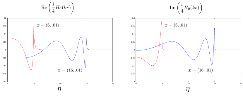
Figure 2: For $k=1$ and source location $\boldsymbol{x}_{0}=(1,.01)$, the plot shows the behavior of the singularity of $H_{0}$ and its dependence on the lateral location of the source and target. The distance $r$ is given by $r~{}=~{}\sqrt{(x-x_{0})^{2}+(y+y_{0}+i\eta)^{2}}$, corresponding to a complex-valued source location.

5 A hybrid approach

It turns out that there is a representation of the impedance Green’s function which can take advantage of both the Sommerfeld integral approach and the method of images. We begin by reconsidering the real image formula (4.7), and separating the image ray into two parts: a near-field component and a far-field component. The scattered field $u$ from formula (4.7) is then written as

$$\begin{split}u(\boldsymbol{x})=&\ g_{k}(\boldsymbol{x},\boldsymbol{x}_{0}-2y_{0}\hat{\boldsymbol{y}})\\ &+2i\alpha\left(\int_{0}^{C}g_{k}(\boldsymbol{x},\boldsymbol{x}_{0}-(2y_{0}-\eta)\hat{\boldsymbol{y}})\,e^{i\alpha\eta}\,d\eta+\int_{C}^{\infty}\!g_{k}(\boldsymbol{x},\boldsymbol{x}_{0}-(2y_{0}-\eta)\hat{\boldsymbol{y}})\,e^{i\alpha\eta}\,d\eta\right),\end{split}$$ (5.1)

where $C$ is a parameter of our choosing. From equations (3.5) and (5.1), it is straightforward to show that

$$\int_{C}^{\infty}g_{k}(\boldsymbol{x},\boldsymbol{x}_{0}-2y_{0}\hat{\boldsymbol{y}}-\eta\hat{\boldsymbol{y}})\,e^{i\alpha\eta}\,d\eta=\frac{1}{4\pi}\int_{-\infty}^{\infty}\frac{e^{-\sqrt{\lambda^{2}-k^{2}}(y+y_{0})}}{\sqrt{\lambda^{2}-k^{2}}}\,\frac{e^{-(\sqrt{\lambda^{2}-k^{2}}-i\alpha)C}}{\sqrt{\lambda^{2}-k^{2}}-i\alpha}\,e^{i\lambda(x-x_{0})}\,d\lambda.$$ (5.2)

This is a Sommerfeld-like formula which, for $C\sim\mathcal{O}(1)$, decays exponentially fast once $\lambda\gtrsim|k|$, independent of $y$ and $y_{0}$. Therefore, the full impedance Green’s function can be written as

$$\begin{split}g_{k,\alpha}(\boldsymbol{x},\boldsymbol{x}_{0})=&\ g_{k}(\boldsymbol{x},\boldsymbol{x}_{0})+g_{k}(\boldsymbol{x},\boldsymbol{x}_{0}-2y_{0}\hat{\boldsymbol{y}})+2i\alpha\int_{0}^{C}g_{k}(\boldsymbol{x},\boldsymbol{x}_{0}-2y_{0}\hat{\boldsymbol{y}}-\eta\hat{\boldsymbol{y}})\,e^{i\alpha\eta}\,d\eta\\ &+\int_{-\infty}^{\infty}\varphi_{k,\alpha,C}(\boldsymbol{x},\boldsymbol{x}_{0},\lambda)\,d\lambda,\end{split}$$ (5.3)

where

$$\varphi_{k,\alpha,C}(\boldsymbol{x},\boldsymbol{x}_{0},\lambda)=\frac{i\alpha}{2\pi}\,\frac{e^{-\sqrt{\lambda^{2}-k^{2}}(y+y_{0})}}{\sqrt{\lambda^{2}-k^{2}}}\frac{e^{-(\sqrt{\lambda^{2}-k^{2}}-i\alpha)C}}{\sqrt{\lambda^{2}-k^{2}}-i\alpha}\,e^{i\lambda(x-x_{0})}\,.$$ (5.4)

Using the previous formula for evaluation, Figure 3 plots (for comparison) the real part of the free-space Green’s function and the impedance half-space Green’s function, for a source located at $(0,5)$ with $k=10.2$.

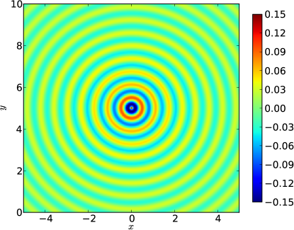
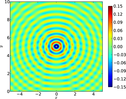
Figure 3: For $k=10.2$, the plot on the left shows the real part of the two dimensional free-space Green’s function and the plot on the right shows the real part of the impedance Green’s function with $\alpha=2.04$. Partial reflection from the boundary $y=0$ is clearly visible.

6 Discretization and fast algorithms

In our numerical experiments, the impedance Green’s function is discretized and evaluated as follows:

$$\begin{split}g_{k,\alpha}(\boldsymbol{x},\boldsymbol{x}_{0})=&g_{k}(\boldsymbol{x},\boldsymbol{x}_{0})+g_{k}(\boldsymbol{x},\boldsymbol{x}_{0}-2y_{0}\hat{\boldsymbol{y}})+\sum_{j=1}^{Q_{I}}v_{j}\,g_{k}(\boldsymbol{x},\boldsymbol{x}_{0}-(2y_{0}+\eta_{j})\hat{\boldsymbol{y}})\\ &+\sum_{j=1}^{Q_{S}}w_{j}\,\varphi_{k,\alpha,C}(\boldsymbol{x},\boldsymbol{x}_{0},\lambda_{j}),\end{split}$$ (6.1)

where $\eta_{j},v_{j}$ represents the $j^{\text{th}}$ quadrature node and weight used in the evaluation of the first integral in (5.3), and $\lambda_{j},w_{j}$ represents the $j^{\text{th}}$ quadrature node and weight used in the evaluation of the second integral in (5.3). Here, $Q_{I}$ and $Q_{S}$ denote the total number of nodes in the discretizations of the first and second integrals, respectively. When the dependence on $\boldsymbol{x}_{0}$ is needed, we will write $Q_{I}(\boldsymbol{x}_{0})$ or $Q_{S}(\boldsymbol{x}_{0})$. The nodes and weights $\{\eta_{j},v_{j}\}$ are chosen to be $16^{\text{th}}$ order Gauss-Legendre nodes on the dyadic subdivisions $[0,2^{-m}C],[2^{-m}C,2^{-m+1}C],\dots,[2^{-1}C,C]$. The number of intervals $(m+1)$ is chosen a priori so that the integral is evaluated to a specified precision $\epsilon$ when $y=0$. Thus, the number of nodes $Q_{I}\approx 16m$. For a scattering source at $(x_{0},y_{0})$, the integral is accurate once the size of the smallest dyadic interval is $\mathcal{O}\left(\frac{y_{0}}{k}\right)$ so that $Q_{I}(\boldsymbol{x}_{0})=\mathcal{O}\left(\log\frac{k}{y_{0}}\right)$. For the Sommerfeld component, the nodes and weights $\lambda_{j},w_{j}$ are chosen to correspond to the trapezoidal rule in the real variable $t\in[-t_{max},t_{max}]$ along the contour

$$\lambda=t-i\tanh t.$$ (6.2)

For $k$ bounded away from zero, this quadrature provides spectral accuracy due to the decay and smoothness of the integrand in the Sommerfeld-like contribution, assuming $t_{max}$ is chosen so that $e^{-(\sqrt{\lambda^{2}-k^{2}}-i\alpha)C}$ is small. This is easy to check and $t_{max}=|k|+20$ is typically sufficient for 10 digits, with the total number of nodes required $Q_{S}$ of the order $\mathcal{O}(k+\alpha)$, assuming $(x-x_{0})=O(1)$. Note that the number of nodes required does not increase as the the distance of the source and target from the interface goes to zero.

Remark 1.

We have not, as yet, specified $C$ from equation (5.1). In all of our experiments, we simply let $C=1$ independent of the source location. In fact, when the source is well separated from the interface (say by a distance of $1/k$, the Sommerfeld integral converges rapidly enough so that the real images aren’t essential.

6.1 A basic fast algorithm

We now sketch an outline of a fast algorithm for evaluating the impedance Green’s function at $N$ targets due to $M$ sources. We denote the $M$ point sources $\{\boldsymbol{x}_{m}^{\prime}\}$ and the $N$ target locations by $\{\boldsymbol{x}_{l}\}$. Thus,

$$u(\boldsymbol{x}_{l})=\sum_{m=1}^{M}c_{m}\,g_{k,\alpha}(\boldsymbol{x}_{l},\boldsymbol{x}_{m}^{\prime})\qquad\text{for $l=1,\ldots,N$}.$$ (6.3)

We proceed in two steps:

1. Compute the first three terms on the right hand side of equation (6.1). These are merely sums of free-space point sources with real coordinates, so their contribution can be computed using a two-dimensional Helmholtz fast multipole method (FMM) in $\mathcal{O}(n\log n)$ time [15, 10, 29], where $n=N+M+M_{image}$. Here, $M_{image}=\sum_{m=1}^{M}Q_{I}(\boldsymbol{x}_{m}^{\prime})$ denotes the total number of image points generated for all sources.

2. Compute the contribution of the Sommerfeld-like integral for each target. A naive calculation would require $\mathcal{O}(NM)$ operations. However, the representation makes it very easy to exploit separation of variables. Denoting by $u_{S}(\boldsymbol{x}_{l})$ the Sommerfeld-like contribution at the point $\boldsymbol{x}_{l}$, and using (5.4), we have

   $$\begin{split}u_{S}(\boldsymbol{x}_{l})&=\sum_{m=1}^{M}c_{m}\sum_{j=1}^{Q_{S}}\,w_{j}\,\varphi_{k,\alpha,C}(\boldsymbol{x},\boldsymbol{x}_{m}^{\prime},\lambda_{j})\\ &=\frac{i\alpha}{2\pi}\sum_{j=1}^{Q_{S}}\,w_{j}\frac{e^{-\sqrt{\lambda_{j}^{2}-k^{2}}y_{l}}}{\sqrt{\lambda_{j}^{2}-k^{2}}}\,\frac{e^{-(\sqrt{\lambda_{j}^{2}-k^{2}}+i\alpha)C}}{\sqrt{\lambda_{j}^{2}-k^{2}}+i\alpha}\,e^{-i\lambda_{j}x_{l}}\,\rho(\lambda_{j},k),\end{split}$$ (6.4)

   where

   $$\rho(\lambda_{j},k)=\sum_{m=1}^{M}c_{m}\,e^{-\sqrt{\lambda_{j}^{2}-k^{2}}y_{m}^{\prime}}\,e^{i\lambda x_{m}^{\prime}}.$$

   The evaluation of $\rho(\lambda_{j},k)$ requires $\mathcal{O}(MQ_{S})$ work. The contribution $u_{S}(\boldsymbol{x}_{l})$ is then computed for each of the $N$ targets using $\mathcal{O}(NQ_{S})$ operations.

Since the number of quadrature nodes $Q_{S}$ is determined by $k$, this part of the algorithm has a net operation count of $\mathcal{O}(nk)$. When $k$ is small, the procedure outlined above is sufficient for a fast algorithm. If $k$ were large, with $n=\mathcal{O}(k)$, a more sophisticated scheme would be required, using either fast multipole or butterfly ideas [16, 10, 28, 29]. This would take us a bit far afield, so we restrict our attention to problems where $n\gg k$. In that regime, the preceding analysis yields a fast $\mathcal{O}(n\log n)$ algorithm for the evaluation of Helmholtz potentials and fields (for fixed values of $k$ and $\alpha$) with impedance half-space boundary conditions.

Tables 4(a) and 4(b) contain timing results for randomly located sources and targets that are either well separated from the interface $y=0$ or located near the interface. The parameters $N$, $M$, and $M_{image}$ are as previously defined. The data in the columns labeled $t_{FMM}$, $t_{SOM}$, and $t_{tot}$ represent the time spent evaluating the free-space FMM, the Sommerfeld-like integrals, and the total time. All experiments were performed using Fortran 90 on a laptop with a $2.53$ GHz Intel Core 2 Duo and 8GB of RAM. The code is not highly optimized, but the timings do demonstrate the approximately linear scaling of our algorithm. Straightforward speedups are possible (e.g. optimizing the location and number of images required, changing the quadrature used in the Sommerfeld-like integral, etc.). The impedance Green’s functions are calculated to absolute precision $\epsilon=10^{-10}$. Note that more images are required when the sources are located near to the interface $y=0$, i.e. the data for $M_{image}$ are larger in Table 4(b) than in Table 4(a). Also, the time required for the Sommerfeld integral portion of the calculation is greater in Table 4(b) than in 4(a). This is because when all the sources and targets are nearer to the interface $y=0$, fewer quadrature nodes can be used in the Sommerfeld integral because the integrand $\varphi_{k,\alpha,C}$ is less oscillatory when $\lambda<k$.

For all the sources in Table 4(a), the images could be omitted as discussed in Remark 1. The same holds true for some portion of the sources in Table 4(b).

6.2 Quadratures for layer potentials

In this section we briefly describe the quadrature scheme we use to compute singular and weakly singular layer potentials of the type that appear in (1.5) and (1.6). For concreteness, we consider the single layer potential $S:L_{2}(\Gamma)\to L_{2}(\Gamma)$:

$$S[\sigma](\boldsymbol{x})=\int_{\Gamma}g_{k,\alpha}(\boldsymbol{x},\boldsymbol{y})\,\sigma(\boldsymbol{y})\,d\boldsymbol{y}(s),$$ (6.5)

where $\boldsymbol{x}\in\Gamma$. Quadrature design for layer potentials is a well-studied problem and there exist many methods for the numerical evaluation such integrals. When the discretization is based upon using equispaced points with respect to some underlying parameterization, corrected trapezoidal rules are very effective [1, 20, 17]. In the two-dimensional case, these schemes can integrate functions with logarithmic singularities to high precision. For each target point $\boldsymbol{x}_{j}\in\Gamma$, they simply add corrections to the quadrature weights for points in the vicinity of $\boldsymbol{x}_{j}$. More precisely, by adding $2k$ corrections, it is possible to obtain errors of the order $O(h^{k})$, where $h$ is the underlying mesh spacing. Better suited for adaptivity are methods based on piecewise high-order approximations of the density $\sigma$ [4, 25, 17, 18]. In this work, we have chosen to use the recently developed QBX method (Quadrature By Expansion) [22], which requires only a high-order quadrature rule for smooth functions. While the method, its analysis, and its implementation are somewhat intricate, the idea is simple.

$N$	$M$	$M_{image}$	$t_{FMM}$	$t_{SOM}$	$t_{tot}$
100	100	12,900	0.56	0.06	0.68
200	200	25,800	1.12	0.12	1.38
400	400	51,600	2.29	0.25	2.80
800	800	103,200	4.78	0.49	5.79
1,600	1,600	206,400	9.68	0.98	11.70
3,200	3,200	412,800	19.43	1.97	23.46
6,400	6,400	825,600	39.21	3.93	47.27

(a) Sources and targets in $(-1,1)\times(2,3)$.

$N$	$M$	$M_{image}$	$t_{FMM}$	$t_{SOM}$	$t_{tot}$
100	100	17,268	0.71	0.03	0.77
200	200	34,920	1.45	0.05	1.57
400	400	70,352	2.95	0.10	3.18
800	800	140,720	6.08	0.21	6.53
1,600	1,600	281,696	12.32	0.41	13.22
3,200	3,200	562,176	25.19	0.83	26.98
6,400	6,400	1,122,960	51.22	1.65	54.79

(b) Sources and targets in $(-1,1)\times(0,1)$.

Figure 4: Timing results for $N$ targets and $M$ sources uniformly randomly distributed, $k=10.2$, and $\alpha=2.04$.

For each target point $\boldsymbol{x}_{j}\in\Gamma$ with normal $\boldsymbol{n}_{j}$, let $\boldsymbol{c}_{j}$ denote a nearby off-surface point, say at

$$\boldsymbol{c}_{j}=\boldsymbol{x}_{j}+r\boldsymbol{n}_{j}.$$

Assuming there are no sources in the disk of radius $r$ about $\boldsymbol{c}_{j}$, $S[\sigma](\boldsymbol{x})$ satisfies the homogeneous Helmholtz equation in that disk. Using the standard separation of variables solution to the Helmholtz equation, we may therefore write

$$S[\sigma](\boldsymbol{x})\approx\sum_{l=-p}^{p}a_{l}\,J_{l}(k\rho)\,e^{-il\theta},$$ (6.6)

where $(\rho,\theta)$ are the polar coordinates of $\boldsymbol{x}$ with respect to the expansion center $\boldsymbol{c}_{j}$ and $J_{l}$ denotes the Bessel function of the first kind of order $l$. Rather than evaluate (6.5) directly, in QBX one evaluates the expansion (6.6) instead. It is shown in [22, 23] that the error in evaluating this local expansion is of the order $\mathcal{O}(r^{p+1}~{}+~{}(\frac{h}{r})^{2q})$, where $h$ is the discretization spacing and $q$ is the order of the underlying quadrature rule for smooth functions. The method converges like a $p^{\text{th}}$-order accurate scheme until the $(\frac{h}{r})^{2q}$ error dominates. This latter term can be made arbitrarily small.

QBX is particularly useful when applied to layer potentials with the impedance half-space Green’s function. If the boundary $\Gamma$ of the obstacle $\Omega$ is very close to the $x$-axis, say within $\epsilon$ of the interface, then the near-field images are located in the lower-half plane at a distance only $2\epsilon$ away. The proximity of these images causes difficulties for standard quadrature techniques because of the near singularities they induce. The QBX expansion centers $\boldsymbol{c}_{j}$, however, may be placed in the interior of $\Omega$, and the integrals are computed easily.

7 Numerical results

We now have the necessary machinery needed to solve non-trivial scattering problems using an integral equation formulation. We discretize the (smooth) scatterer at equispaced points with respect to the underlying parameterization, and, unless otherwise noted, use a $16^{\text{th}}$-order QBX quadrature scheme to evaluate layer potentials. We solve the discretized integral equation using the iterative method GMRES, accelerated by the fast algorithm described in Section 6.1.

The numerical examples in this section illustrate the accuracy of the computation of $g_{k,\alpha}$, as well as the robustness of our hybrid representation with respect to the location of the sources and targets (in particular, when both source and target are located near the interface $y=0$).

We first solve the exterior (sound-soft) Dirichlet problem with impedance interface conditions:

$$\begin{split}(\triangle+k^{2})u^{tot}(\boldsymbol{x})=\delta(\boldsymbol{x}-\boldsymbol{x}_{0})&\qquad\text{in }P\setminus\Omega,\\ \frac{\partial u^{tot}}{\partial n}-i\alpha u^{tot}=0&\qquad\text{on }y=0,\\ u^{tot}=0&\qquad\text{on }\Gamma,\end{split}$$ (7.1)

where $\Omega$ is an inclusion in the interior of the upper half-space. We assume a representation of the scattered field in the form of a double layer potential:

$$u(\boldsymbol{x})=\int_{\Gamma}\left[\frac{\partial}{\partial n_{y}}g_{k,\alpha}(\boldsymbol{x},\boldsymbol{y})\right]\sigma(\boldsymbol{y})\,d\boldsymbol{y}(s),$$ (7.2)

where as before $u^{tot}=u+u^{in}$. This representation leads to the integral equation

$$\frac{1}{2}\sigma(\boldsymbol{x})+\int_{\Gamma}\left[\frac{\partial}{\partial n_{y}}g_{k,\alpha}(\boldsymbol{x},\boldsymbol{y})\right]\sigma(\boldsymbol{y})\,d\boldsymbol{y}(s)=-u^{in}(\boldsymbol{x}),$$ (7.3)

which is a Fredholm equation of the second-kind, with the integral interpreted in the principal value sense. The equation (7.3), like (1.6), is invertible except for a countable sequence of spurious resonances. Rather than use a more complicated, resonance-free representation, we assume $k$ is not a spurious resonance. See [6] for a thorough discussion of integral equations in the impedance scattering context. Figures 5(a) and 5(b) show the total potential in the exterior of the scatterer $\Omega$ with zero Dirichlet conditions. In these, and the subsequent Neumann scattering examples, the boundary of the scatterer, $\Gamma$, is described by the curve $\gamma:[0,2\pi]\to\mathbb{R}^{2}$, where $\gamma(t)=(x(t),y(t))$ and

$$\begin{split}x(t)&=1.1+(1+0.2\cos{4t})\cos{t},\\ y(t)&=1.2+\delta+(1+0.2\cos{4t})\sin{t}.\end{split}$$ (7.4)

The magnitude $\delta$ of the distance to the interface $y=0$ is indicated below below each figure. Accuracy results are given in Table 1. Note that more discretization points were required when $\delta=10^{-3}$, i.e. when the scatterer is close to the impedance boundary. An adaptive discretization scheme, instead of a global trapezoidal rule, would result in many fewer nodes. A slightly higher-order quadrature, $20^{\text{th}}$-order, was used in the $\delta=10^{-3}$ case.

	Dirichlet, $\delta=0.8$	Dirichlet, $\delta=10^{-3}$	Neumann, $\delta=0.8$	Neumann, $\delta=10^{-3}$
Number of points	500	1500	500	1500
Rel. error at target $u$	0.10E-9	0.15E-10	0.22E-9	0.14E-11
Rel. $L_{2}$ error of $\sigma$	0.29E-9	0.32E-10	0.40E-9	0.98E-8
$L_{2}$ norm of $\sigma$	2.13	2.95	4.03	3.50

Table 1: Accuracy results.

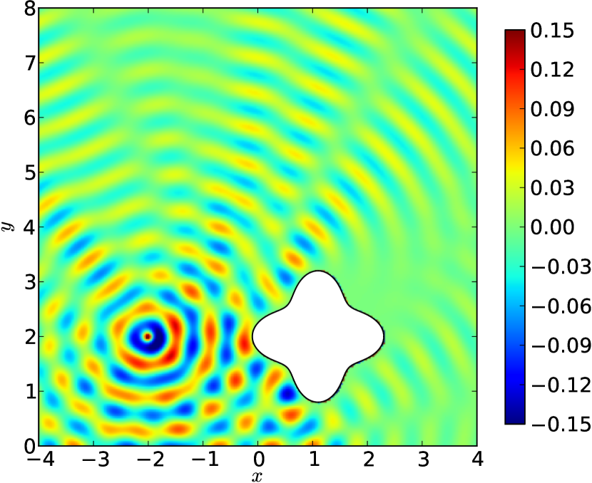
(a) Exterior Dirichlet, $\delta=0.8$.

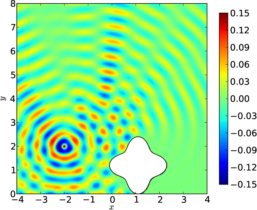
(b) Exterior Dirichlet, $\delta=10^{-3}$.

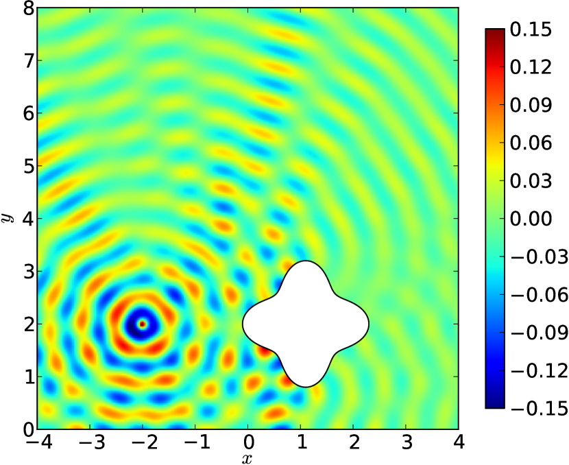
(c) Exterior Neumann, $\delta=0.8$.

(d) Exterior Neumann, $\delta=10^{-3}$.

Figure 5: For $k=10.2$ and $\alpha=2.04$, we show the real part of the total field for exterior Dirichlet and Neumann problems. The incoming field in all cases is due to a unit strength impedance point source located at $(-2,2)$. The distance of the scatterer from the interface is listed below each figure.

In the second set of experiments, we solve the exterior (sound-hard) Neumann problem with impedance half-space conditions:

$$\begin{split}(\triangle+k^{2})u^{tot}(\boldsymbol{x})=\delta(\boldsymbol{x}-\boldsymbol{x}_{0})&\qquad\text{in }P\setminus\Omega,\\ \frac{\partial u^{tot}}{\partial n}-i\alpha u^{tot}=0&\qquad\text{on }y=0,\\ \frac{\partial u^{tot}}{\partial n}=0&\qquad\text{on }\Gamma.\end{split}$$ (7.5)

As discussed in the introduction, we represent the scattered field by a single layer potential (1.5), yielding the integral equation (1.6). Figures 5(c) and 5(d) show the total potential in the exterior of the scatterer $\Omega$.

It is worth repeating that the interface $y=0$ does not need to be discretized because of the use of the impedance Green’s function $g_{k,\alpha}$. The number of discretization points and quadrature parameters for our examples were not carefully chosen. They were simply chosen to be sufficiently fine to yield an estimated precision in the scattered field of $10^{-10}$. The impedance Green’s function was evaluated to absolute precision $10^{-11}$ and the GMRES residual tolerance was set to $10^{-10}$. Our goal here is simply to demonstrate the accuracy and robustness of our hybrid representation of the Green’s function.

The accuracy of the solvers is tested by two different methods. First, a unit strength source is placed at a point $\boldsymbol{x}_{I}$ in the interior of the scatterer $\Omega$. The function $g_{k,\alpha}(\boldsymbol{x},\boldsymbol{x}_{I})$ is then a known exact solution satisfying the homogeneous Helmholtz equation in $P\setminus\Omega$. Using the Dirichlet or Neumann data corresponding to $g_{k,\alpha}(\boldsymbol{x},\boldsymbol{x}_{I})$, we can solve the boundary integral equations (1.6) and (7.3) and compare the computed solution at target points in $P\setminus\Omega$ with the known exact solution. For the true scattering problem, the source is exterior to $\Omega$ and an exact solution is not available in closed form. In this case, we carry out a self-consistent convergence test. That is, the number of discretization points is doubled and the relative $L_{2}$ error is calculated with the finer grid solution used as the reference solution. The error in the potential at a target point in the exterior of $\Omega$ is calculated in the same fashion. Results of the self-consistent convergence tests are shown in Table 1. The location of the target point in the exterior at which the value of the potential was computed is $(0,5)$ in all examples.

7.1 Scattering from a locally perturbed half-space

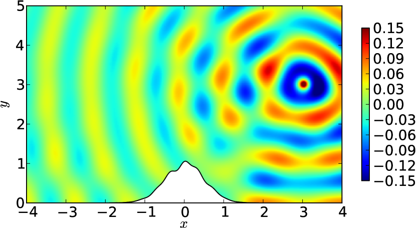
(a) Impedance scattering from a half-space perturbation.

Number of points	4,000
Rel. $L_{\infty}$ error of $u$	0.40E-9
Rel. $L_{2}$ error of $\sigma$	0.51E-8
$L_{2}$ norm of $\sigma$	0.76

(b) Accuracy results.

Figure 6: The real part of the total potential is plotted for $k=5.7$ and $\alpha=.855$ over a perturbed impedance half-space. The incoming field is due to a unit strength point source located at $(3,3)$. Accuracy results are obtained by doubling the number of discretization points, for a test target point located at $(-2,4)$.

Lastly, we demonstrate the use of the impedance Green’s function in solving the problem of scattering from a half-space which contains a local perturbation. A thorough analysis can be found in [9]. Here, we simply consider one such example. We let $\Omega$ denote the region below the curve $\gamma_{1}:(-\infty,\infty)\to\mathbb{R}^{2}$, where $\gamma_{1}(t)=(x(t),y(t))$ and

$$\begin{split}x(t)&=t,\\ y(t)&=\left(1+0.05\left(\sin 8.79t+\cos 16.96t+\sin 1.88t\right)\right)\,e^{-2t^{2}}.\end{split}$$ (7.6)

For values of $t$ outside the interval $[-4,4]$, $|y(t)|<2.0\times 10^{-14}$. Therefore, $\gamma_{1}$ is only discretized for $t\in[-4,4]$, outside of which it is indistinguishable (to machine precision) from the interface $y=0$. Thus, outside of $t\in[-4,4]$, the impedance condition is automatically satisfied to machine precision if the appropriate Green’s function is used to represent the solution. On the half-space perturbation $\Gamma=\{\gamma_{1}(t),t\in[-4,4]\}$, we must enforce the desired impedance condition:

$$\frac{\partial u^{tot}}{\partial n}-i\alpha u^{tot}=0\qquad\text{on }\Gamma,$$ (7.7)

where $n=(y^{\prime},-x^{\prime})$ is a unit normal vector pointing into the lower half space $\Omega$. In short, we seek to solve the boundary value problem:

$$\begin{split}(\triangle+k^{2})u^{tot}(\boldsymbol{x})=\delta(\boldsymbol{x}-\boldsymbol{x}_{0})&\qquad\text{in }P\setminus\Omega,\\ \frac{\partial u^{tot}}{\partial n}-i\alpha u^{tot}=0&\qquad\text{on }\Gamma.\end{split}$$ (7.8)

We assume an integral representation for the scattered field $u$:

$$u(\boldsymbol{x})=\int_{\Gamma}g_{k,\alpha}(\boldsymbol{x},\boldsymbol{y})\,\sigma(\boldsymbol{y})\,d\boldsymbol{y}(s),$$ (7.9)

which results in the integral equation

$$\frac{1}{2}\sigma(\boldsymbol{x})+\int_{\Gamma}\left[\frac{\partial}{\partial n_{x}}g_{k,\alpha}(\boldsymbol{x},\boldsymbol{y})\right]\sigma(\boldsymbol{y})\,d\boldsymbol{y}(s)-i\alpha\int_{\Gamma}g_{k,\alpha}(\boldsymbol{x},\boldsymbol{y})\,\sigma(\boldsymbol{y})\,d\boldsymbol{y}(s)=-\frac{\partial u^{in}(\boldsymbol{x})}{\partial n_{x}}+i\alpha u^{in}(\boldsymbol{x}).$$ (7.10)

This is a simplification of the integral equation approach discussed in [9], which addresses the more general case of a half-space perturbation that is allowed to deviate both above and below the interface $y=0$. For simplicity, we have assumed that the perturbation $\gamma_{1}$ satisfies $y(t)\geq 0$.

Even though the curve $\gamma_{1}$ in this half-space scattering example comes arbitrarily close to the interface $y=0$, we obtain high accuracy (using a $16^{\text{th}}$ order QBX scheme with the trapezoidal rule as the underlying smooth rule). The reason for this is that the density $\sigma$ decays exponentially as $|t|$ increases and is as smooth as the perturbation itself. Unlike the closely-touching Dirichlet and Neumann scattering problems, the half-space perturbation problem is not physically ill-conditioned.

Figure 6 shows the real part of the total potential $u^{tot}$. The incoming potential is due to an impedance point source located at $(3,3)$, and the error in the total potential is calculated at $(-2,4)$. Errors are calculated in the same manner as for the Dirichlet and Neumann scattering examples, using a self-consistent convergence test.

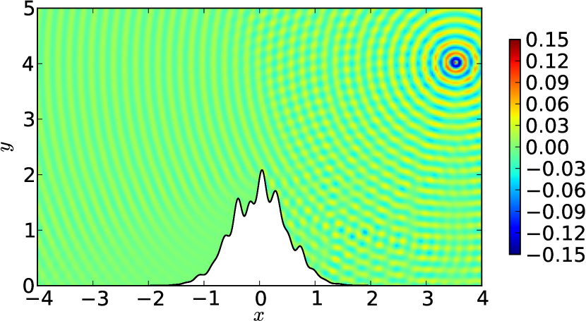
(a) Impedance scattering from a half-space perturbation.

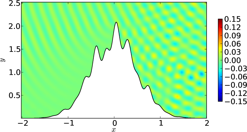
(b) A closer view.

Figure 7: The real part of the total potential is plotted for $k=31.7$ and $\alpha=5.389$ over a perturbed impedance half-space. The incoming field is due to a unit strength point source located at $(3.5,4)$. The perturbation was discretized with $20,000$ points, and a relative $L_{2}$ error of $10^{-5}$ was obtained in the density $\sigma$ and $10^{-7}$ in $u^{tot}$ at $(-2,5)$. The deviation is approximately $60$ wavelengths long.

Figure 7 shows the real part of the total potential $u^{tot}$ for a higher value of the wavenumber $k$ than Figure 6, and a more complicated perturbation $\gamma_{2}(t)=(x(t),y(t))$ with

$$\begin{split}x(t)&=t,\\ y(t)&=\left(1.75+\frac{1}{6}\left(\sin 8.79t+\cos 16.96t+\sin 27.02t+\frac{1}{7}\cos 32.67t\right)\right)\,e^{-2t^{2}}.\end{split}$$ (7.11)

The incoming potential is due to an impedance point source slightly farther away, located at $(3.5,4)$, and the error in the total potential is calculated at $(-2,5)$. Errors are calculated as previously discussed.

8 Conclusions

We have derived a new formula for the half-space Helmholtz Green’s function satisfying impedance boundary conditions in two dimensions. The representation (5.3) consists of a free-space Helmholtz Green’s function in the upper half-space, a short segment of images in the lower half-space with real coordinates, and a rapidly converging Sommerfeld-like integral. Unlike the method of complex images, it is straightforward to accelerate with an FMM using a modest number of discrete image charges. The impedance Green’s function is easily evaluated to full double-precision accuracy, insensitive (within logarithmic factors) to the location of the source and target, using a modest number of operations that depends only on $k$ and $\alpha$.

Although we have carried out a detailed derivation only for the two-dimensional case, the results are nearly identical in three dimensions. Using the three-dimensional Green’s function $g_{k}(\boldsymbol{x},\boldsymbol{y})=-\frac{e^{ik|\boldsymbol{x}-\boldsymbol{y}|}}{4\pi|\boldsymbol{x}-\boldsymbol{y}|}$, it is straightforward to show that

$$\begin{split}g_{k,\alpha}(\boldsymbol{x},\boldsymbol{x}_{0})=&\ g_{k}(\boldsymbol{x},\boldsymbol{x}_{0})+g_{k}(\boldsymbol{x},\boldsymbol{x}_{0}-2y_{0}\hat{\boldsymbol{y}})+2i\alpha\int_{0}^{C}g_{k}(\boldsymbol{x},\boldsymbol{x}_{0}-(2y_{0}+\eta)\hat{\boldsymbol{y}})\,e^{-i\alpha\eta}\,d\eta\\ &+\frac{i\alpha}{2\pi}\int_{-\infty}^{\infty}\frac{e^{-\sqrt{\lambda^{2}-k^{2}}(y+y_{0})}}{\sqrt{\lambda^{2}-k^{2}}}\frac{e^{-(\sqrt{\lambda^{2}-k^{2}}+i\alpha)C}}{\sqrt{\lambda^{2}-k^{2}}+i\alpha}J_{0}(\lambda r)\,d\lambda,\end{split}$$ (8.1)

where $J_{0}$ is the zeroth-order Bessel function of the first kind.

A more complicated extension of our approach is to the evaluation of the layered medium Green’s function, where each layer has a distinct Helmholtz coefficient and various (application-dependent) continuity conditions are imposed across each layer. In this case, an explicit real image structure is not available via the Laplace transform. We are currently investigating a semi-numerical approach that appears promising. We are also developing hybrid representations for the full Maxwell equations with impedance boundary conditions [27].

The reader may have noted that formulas (5.1) and (5.3) make use of a discrete image at $(x_{0},-y_{0})$ with the same sign as the original source. As $\alpha\rightarrow 0$, the impedance condition becomes a sound-hard condition and the discrete image is all that remains, as one would expect. As $|\alpha|\rightarrow\infty$, however, the limit of the impedance condition is a Dirichlet condition, while the image formula diverges. One should expect to see a simple image source at $(x_{0},-y_{0})$ with the opposite sign. This is easy to accomplish by using a complementary image formula. Rather than (4.4), one can write

$$\begin{split}\int_{0}^{\infty}e^{-\sqrt{\lambda^{2}-k^{2}}\eta}\,\tau(\eta)\,d\eta&=\frac{\sqrt{\lambda^{2}-k^{2}}-i\alpha}{\sqrt{\lambda^{2}-k^{2}}+i\alpha}\\ &=-1+\frac{2\sqrt{\lambda^{2}-k^{2}}}{\sqrt{\lambda^{2}-k^{2}}+i\alpha}\,.\end{split}$$ (8.2)

This has the desired asymptotic behavior as $\alpha\rightarrow\infty$. In applications $\alpha$ is typically $\mathcal{O}(|k|)$, and the formula presented in Section 5 serves its purpose well.

References

- [1] B. Alpert. Hybrid Gauss-trapezoidal quadrature rules. SIAM J. Sci. Comput., 20(5):1551–1584, 1999.
- [2] K. Attenborough. Acoustical impedance models for outdoor ground surfaces. J. Sound Vib., 99(4):521–544, 1985.
- [3] A. Barnett and L. Greengard. A new integral representation for quasi-periodic scattering problems in two dimensions. BIT Numer. Math., 51(1):67–90, 2011.
- [4] J. Bremer, Z. Gimbutas, and V. Rokhlin. A nonlinear optimization procedure for generalized Gaussian quadratures. SIAM J. Sci. Comput., 32(4):1761–1788, 2010.
- [5] W. Cai and T. J. Yu. Fast Calculations of Dyadic Green’s Functions for Electromagnetic Scattering in a Multilayered Medium. J. Comput. Phys., 165(1):1–21, 2000.
- [6] S. N. Chandler-Wilde. The impedance boundary value problem for the Helmholtz equation in a half-plane. Math. Methods Appl. Sci., 20(10):813–840, 1997.
- [7] S. N. Chandler-Wilde and K. V. Horoshenkov. Padé approximants for the acoustical characteristics of rigid frame porous media. J. Acoust. Soc. Am., 98(2):1119–1129, 1995.
- [8] S. N. Chandler-Wilde and D. C. Hothersall. Efficient calculation of the Green function for acoustic propagation above a homogeneous impedance plane. J. Sound Vib., 180(5):705–724, 1995.
- [9] S. N. Chandler-Wilde and A. T. Peplow. A boundary integral equation formulation for the Helmholtz equation in a locally perturbed half-plane. J. Appl. Math. Mech., 85(2):79–88, 2005.
- [10] H. Cheng, W. Y. Crutchfield, Z. Gimbutas, J. H. L. Greengard, V. Rokhlin, N. Yarvin, and J. Zhao. Remarks on the implementation of the wideband FMM for the Helmholtz equation in two dimensions. Contemp. Math., 408:99–110, 2006.
- [11] D. Colton and R. Kress. Integral Equation Methods in Scattering Theory. John Wiley & Sons, Inc., 1983.
- [12] X. Di and K. Gilbert. An exact Laplace transform formulation for a point source above a ground surface. J. Acoust. Soc. Amer., 93(2):714–720, 2000.
- [13] F. DiNapoli and R. Deavenport. Theoretical and numerical Green’s function field solution in a plane multilayered medium. J. Acoust. Soc. Amer., 67(1):92–105, 1980.
- [14] M. Duran, R. Hein, and J.-C. Nedelec. Computing numerically the Green’s function of the half-plane Helmholtz operator with impedance boundary conditions. Numer. Math., 107(2):295–314, 2007.
- [15] Z. Gimbutas and L. Greengard. FMMLIB2D, April 2012. v. 1.2, available at www.cims.nyu.edu/cmcl.
- [16] L. Greengard, J. Huang, V. Rokhlin, and S. Wandzura. Accelerating Fast Multipole Methods for the Helmholtz Equation at Low Frequencies. IEEE Comput. Sci. Eng., 5(3):32–38, 1998.
- [17] S. Hao, P.-G. Martinsson, and P. Young. High-order accurate Nystrom discretization of integral equations with weakly singular kernels on smooth curves in the plane. arXiv, 1112.6262/math.NA, 2011.
- [18] J. Helsing and R. Ojala. Corner singularities for elliptic problems: Integral equations, graded meshes, quadrature, and compressed inverse preconditioning. J. Comput. Phys., 227(20):8820–8840, 2008.
- [19] A. Hochmann and Y. Leviatan. A numerical methodology for efficient evaluation of 2D Sommerfeld integrals in the dielectric half-space problem. IEEE Trans. Antennas and Propagation, 58(2):413–431, 2010.
- [20] S. Kapur and V. Rokhlin. High-order corrected trapezoidal quadrature rules for singular functions. SIAM J. Numer. Anal., 34(4):1331–1356, 1997.
- [21] O. D. Kellogg. Foundations of Potential Theory. Dover Publications, Inc., New York, New York, 1954.
- [22] A. Klöckner, A. Barnett, L. Greengard, and M. O’Neil. Quadrature by Expansion: A New Method for the Evaluation of Layer Potentials. arxiv, 1207.4461/math.NA, 2012. Submitted.
- [23] A. Klöckner, L. Greengard, and M. O’Neil. Fast algorithms for the evaluation of layer potentials using Quadrature by Expansion. In preparation.
- [24] I.-S. Koh and J.-G. Yook. Exact Closed-Form Expression of a Sommerfeld Integral for the Impedance Plane Problem. IEEE Trans. Antennas and Propagation, 54(9):2568–2576, 2006.
- [25] P. Kolm and V. Rokhlin. Numerical quadratures for singular and hypersingular integrals. Comput. Math. Appl., 41(3–4):327–352, 2001.
- [26] M. Ochmann. The complex equivalent source method for sound propagation over an impedance plane. J. Acoust. Soc. Amer., 116(6):3304–3311, 2004.
- [27] M. O’Neil and J. Sifuentes. Acoustic scattering in three dimensions with half-space impedance boundary conditions. In preparation.
- [28] M. O’Neil, F. Woolfe, and V. Rokhlin. An algorithm for the rapid evaluation of special function transforms. Appl. Comput. Harmon. Anal., 41(2):203–226, 2010.
- [29] V. Rokhlin. Rapid Solution of Integral Equations of Scattering Theory in Two Dimensions. J. Comput. Phys., 86(2):414–439, 1990.
- [30] K. Sarabandi and I.-S. Koh. Fast Multipole Representation of Green’s Function for an Impedance Half-Space. IEEE Trans. Antennas and Propagation, 52(1):296–301, January 2004.
- [31] A. Sommerfeld. Uber die ausbreitung der wellen in der drahtlosen telegraphie. Ann. Phys. Leipzig, 28:665–737, 1909.
- [32] G. Taraldsen. The complex image method. Wave Motion, 43(1):91–97, 2005.
- [33] B. Van der Pol. Theory of the reflection of the light from a point source by a finitely conducting flat mirror, with an application to radiotelegraphy. Physica, 2(1–12):843–853, 1935.
- [34] H. Weyl. Ausbreitung elektromagnetischer wellen uber einem ebenen leiter. Ann. Phys. Leipzig, 60:481–500, 1919.