Observations of Post-flare Plasma Dynamics during an M1.0 Flare in AR11093 by SDO/AIA*

Abstract

We observe the motion of cool and hot plasma in a multi-stranded post flare loop system that evolved in the decay phase of a two ribbon M1.0 class flare in AR 11093 on 7 August 2010 using SDO/AIA 304 Å and 171 Å filters. The moving intensity feature and its reflected counterpart are observed in the loop system at multi-temperature. The observed hot counterpart of the plasma that probably envelopes the cool confined plasma, moves comparatively faster ($\sim$34 km s^-1) to the later (29 km s^-1) in form of the spreaded intensity feature. The propagating plasma and intensity reflect from the region of another footpoint of the loop. The subsonic speed of the moving plasma and associated intensity feature may be most likely evolved in the post flare loop system through impulsive flare heating processes. Complementing our observations of moving multi-temperature intensity features in the post flare loop system and its reflection, we also attempt to solve two-dimensional ideal magnetohydrodynamic equations numerically using the VAL-IIIC atmosphere as an initial condition to simulate the observed plasma dynamics. We consider a localized thermal pulse impulsively generated near one footpoint of the loop system during the flare processes, which is launched along the magnetic field lines at the solar chromosphere. The pulse steepens into a slow shock at higher altitudes while moving along this loop system, which triggers plasma perturbations that closely exhibit the observed plasma dynamics.

1 Introduction

Post flare loops are the dynamic and transient loop systems that evolve in flaring active regions , and exhibit strong localized heating and cooling effects, as well as emissions in various parts of the electromagnetic spectrum (e.g., HXR, SXR, EUV, H_α) during the gradual reconnection process occurred in the flare activity (Harra-Murnion et al., 1998; Reeves & Warren, 2002; Li & Zhang, 2009a). Recently, Cheng et al. (2010) have observed a re-flaring event in the evolved post flare loop system triggered by the magnetic flux emergence. Li & Zhang (2009b) have observed the brightness propagation in post flare loop (PFLs) systems. They have investigated that the dynamics of these brightened PFLs were along the neutral lines and separation of the flare ribbons were perpendicular to the neutral lines. Their observations indicate that the footpoints of the initially brightened PFLs were always associated with the change of the photospheric magnetic fields, and support the general 3-D model of the magnetic reconnection (Shiota et al., 2005). Warren et al. (1999) have observed impulsive footpoint brightening in a two ribbon flare followed by the formation of high-temperature plasma in the corona and then cooler post flare loops below the hot plasma, which also supports the standard reconnection model of solar flares. There are several mechanisms to understand the heating of post flare loops in which the most likely mechanism of their heating and rise-up may be attributed to slow magnetohydrodynamic shock waves (Cargill & Priest, 1982). Recently, Fernández et al. (2009) have numerically simulated the internal plasma dynamics in such post flare loops, and concluded that the high-speed downflow perturbations, usually interpreted as slow magnetoacoustic waves before, could now be interpreted as slow magnetoacoustic shock waves. Longcope et al. (2009) have also reported the field lines shortening in post flare loop system and inferred the localized, three-dimensional reconnection to heat the plasma. The shortening progresses away from the reconnection location with an Alfvén speed and release magnetic energy and generate parallel compressive flows.

The post-flare loops are not only the most dynamic magnetic flux tubes associated with heating, cooling, and mass flows, but also the excellent waveguides for the excitation of various types of magnetohydrodynamic waves and oscillations. O’Shea et al. (2007) have observed the simultaneous presence of propagating disturbances and multiple harmonics of the fast magnetoacoustic kink oscillations in the transition region post flare loops in their cooling phase. Srivastava et al. (2008) have also observed the multiple harmonics of the sausage oscillations in the cool post flare loops along with a strong downflow of the plasma. Recently, Nakariakov & Zimovets (2011) have reported the propagating disturbances in the loop system associated with two-ribbon flare as a signature of slow magnetoacoustic waves. Moreover, Kryshtal & Gerasimenko (2004) have found that two types of waves are generated in post flare loops due to the growth of instabilities, e.g., the kinetic Alfvén-like waves and magnetoacoustic waves. The observations of waves and oscillations in the highly dynamic post flare loops provide compelling motivation to diagnose their crucial plasma properties using principle of MHD seismology to understand its dynamics (Andries et al., 2009; Aschwanden, 2009; Macnamara & Roberts, 2010, 2011; Srivastava, 2010, and references cited there).

In the present paper, we present the recent SDO/AIA observations of the moving intensity features seen in a multi-temperature plasma in a multi-stranded post flare loop system whose footpoints are anchored in the two opposite magnetic polarities at two flare ribbons. We do not aim to study the large-scale post flare loop dynamics during whole long duration decay phase of the associated M-class flare in AR11093 on 7 August 2010. However, we do aim to analyse the most probable cause of the internal dynamics of the moving intensity feature and its reflection in the loop system during 15 minutes (18:44 UT-18:58 UT) when it was almost in equilibrium. In an attempt to understand the dynamics and plasma conditions of the observed post flare loop system that is rather complex, we numerically model the plasma dynamics by solving 2-D ideal MHD equations using the VAL III C thermodynamic structure as an initial condition by triggerring a thermal pulse near one footpoint of the simulated loop system. Our numerical model provides only a rough guide for the observed complex plasma dynamics as it does not include thermal condution and radiative cooling . In the present paper we mainly focus on the unique observations of the post flare plasma dynamics during an M-class flare, but we also briefly present the supportive results of munerical modeling that approximately exhibit the observed internal plasma dynamics. In Sec. 2, we present observations and results. We describe the numerical models in Sec. 3. In Sec. 4, we report the results of numerical simulations. The discussion and conclusions are given in the last section.

2 Observations and Results

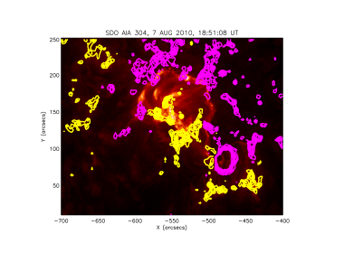
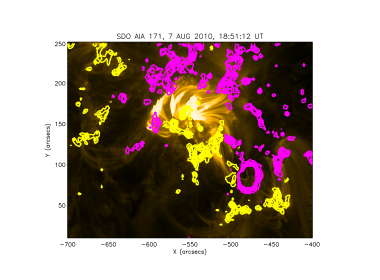
Figure 1: The enlarged field-of-view of the two-ribbons and a post flare phase of an M1.0 class flare in AR11093 are shown at 18:51 UT on 7 August 2010 as observed by SDO/AIA 304 Å (left-panel) and 171 Å (right-panel). The SoHO/MDI magnetic polarities are over-plotted above these snapshots that clearly reveal the opposite field distributions (+ve with yellow and -ve with magenta) at the two flare ribbons. The contour levels are with $\pm{800}$ G magnetic field strength.

We use the time series data of post flare phase of a two ribbon M1.0 class solar flare in AR11093 on 7 August 2010 as observed in a 304 Å and 171 Å filters of the Atmospheric Assembly Imager (AIA) onboard Solar Dynamics Observatory (SDO) on 7 August 2010. Although the AR 11093 evolution and M1.0 class flare are observed by all the SDO/AIA filters as well as other instruments (e.g., STEREO-B, SoHO/EIT, MDI etc), we present the high-resolution SDO/AIA observations of the evolution of a post flare loop system during 18:44 UT-18:58 UT in just two filters 304 Å and 171 Å in order to study the unique post flare multi-temperature internal plasma dynamics. These two filters represent the plasma emissions formed respectively at temperatures $\sim$0.1 MK and $\sim$1.0 MK. The SDO/AIA has a typical resolution of 0.6$"$ per pixel and the highest cadence of 12 s, and it observes the full solar disk in three UV (1600 Å, 1700Å, 4500 Å) and seven EUV (171 Å, 193 Å, 211 Å, 94 Å, 304 Å, 335 Å, 131 Å) lines (Lemen et al., 2011). In Fig.1, the enlarged field-of-view of the two-ribbons and post flare phase of an M1.0 class flare in AR11093 are shown at 18:51 UT on 7 August 2010 as observed by SDO/AIA 304 Å (left-panel) and 171 Å (right-panel). The SoHO/MDI magnetic polarities are over plotted above these snap-shots that clearly reveal the opposite field distributions (+ve with yellow and -ve with magenta) over the two flare ribbons. The MDI contour levels are $\pm$800 G of the magnetic field strength. The time series has been obtained by the SSW cutout service at LMSAL, USA, which is corrected for the flat-field and spikes. We run aia_prep subroutine of SSW IDL for further calibration and cleaning of the time series data.

As per Hinode/EIS flare catalog ,the M1.0 class flare begins in AR 11093 (N11^o E34^o) on $\sim$17:55 UT, peaks at $\sim$18:24 UT, and subsided on $\sim$18:47 UT. However, as per GOES X-ray flux measurements, its decay phase is extended upto $\sim$20:50 UT making it almost a long duration event (LDE). A part of huge and twisted filament that was aligned along the magnetic neutral line, rose and erupted. The activated flux-rope and its reconnection with the overlying coronal loops may most likely begin the flare energy release process. The detailed morphological study of this M1.0 class flare and associated CME has been recently reported by Reddy et al. (2011). The transient brightening of the two ribbons occurred due to the precipitation of energetic particles towards the loop footpoints that participated in gradual reconnection process in the corona. Therefore, the heating of the low atmospheric plasma along the two ribbons uploads the mass and forms a new set of the post flare loops in the decay phase of the flare (cf., Fig. 1). In this paper, we aim only to study the short duration internal plasma dynamics of a post flare loop system during M1.0 class flare in the observations.

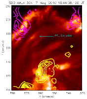
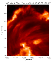
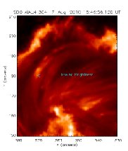
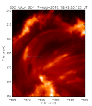
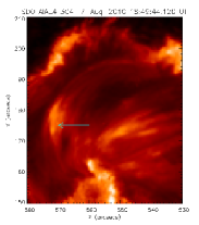
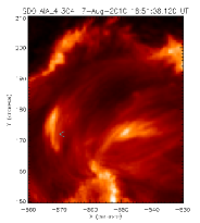
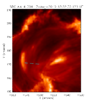
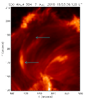
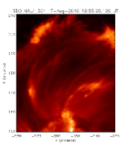
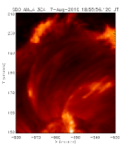
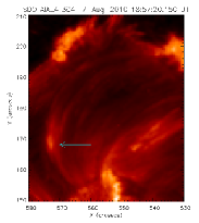
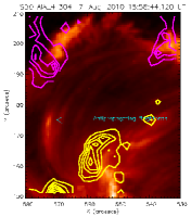
Figure 2: The time sequence of a selected multi-stranded post flare loop system showing complex plasma dynamics during 18:44 UT-18:58 UT. .The loop system and cool counter part of the bright denser plasma ($\sim$0.1 MK) are evolved on 18:44 UT. The brightness propagates downward towards southward footpoint (18:44-18:55 UT) of the loop system and then reflects again in the northward direction (18:58 UT) as an antipropagating brightness.

In Fig. 2, we observe a very unique evolution of multi-stranded post flare loop system on 18:44 UT. A moving intensity feature is clearly evident in the loop system on 18:46 UT, which propagates down towards southward footpoint of the loop system. It gradually brightens and moves downward till 18:52 UT, and thereafter, it still propagates downward with a subsequent decrease in its intensity. It is not confined in one strand, but seems to propagate in the multiple strands of the post flare loop system. The southward positive polarity footpoint (yellow MDI contours) and northward negative polarity footpoint (magenta MDI contours) of the loop system are plotted in the first and last snapshots of Fig. 2. The contour levels are with $\pm{800}$ G magnetic field strength. The multiple strands of the loop system are clearly anchored in these two foot points. We estimate the approximate lower bound velocity of this moving intensity feature as $\sim$29 km s^-1. This is a sub-sonic speed as the local sound speed at the formation temperature (T_f$\sim$1$\times$$10^{5}$ K) of He II ion that emits 304 Å , is around 46 km s^-1. The interesting scenario became evident in form of the antipropagation of moving intensity during 18:57-18:58 UT, which indicates the reflection of this low temperature counterpart of the plasma near the southward footpoint of the post flare loop system. However, it should be noted that the moving intensity feature could not exactly reach to the southward footpoint of loop, but it started reflecting back from its nearby location.

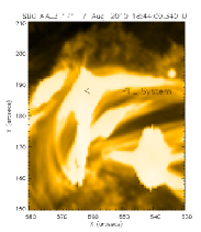
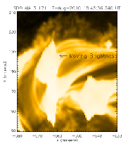
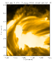
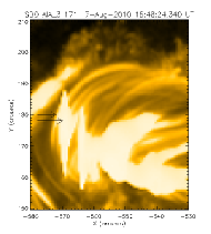
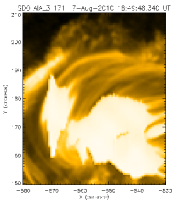
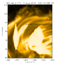
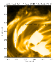
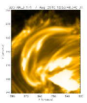
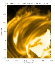
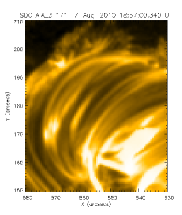
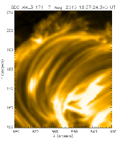
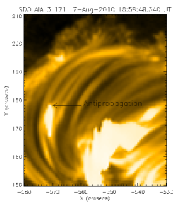
Figure 3: The time sequence of a selected multi-stranded post flare loop system showing complex plasma dynamics during 18:44 UT-18:58 UT. .The loop system and hot counter part of the bright denser plasma ($\sim$1.0 MK) are evolved on 18:44 UT. The brightness propagates downward towards southward footpoint of the loop system and then reflects again in the northward direction as an antipropagating brightness.

In Fig. 3, we also observe this very unique evolution of multi-stranded post flare loop system at coronal temperature ($\sim$1.0 MK) in 171 Å filter of SDO/AIA. The bright post flare loop system is clearly appeared on 18:44 UT. A brightness associated with high temperature counterpart of the plasma, however, is spreaded over the larger regions in the post flare loop system and clearly evident on 18:45 UT. This means that the high temperature counterpart of the plasma envelopes its low temperature counterpart and form the co-spatial multitemperature plasma blob. The high temperature counterpart of the moving intensity propagates down towards southward footpoint of the loop system. It gradually brightens and moves downward till 18:51 UT, and thereafter it still propagates downward with decreasing intensity. It is clearly visible in the coronal image on 18:51 UT that the near footpoints areas of these multiple strands are merged with each other and forming a multiple stranded post flare loop system. The brightness is not confined in one strand, but it seems to propagate in multiple strands of the post flare loop system. We estimate the approximate lower bound velocity of this moving intensity feature as $\sim$34 km s^-1. This is a sub-sonic speed as the local sound speed at the formation temperature (T${}_{f}\sim$1.0 MK) of Fe IX ion that emits 171 Å, is $\sim$147 km s^-1. The interesting scenario became evident again in form of the antipropagation of the moving intensity during 18:51-18:58 UT in various parts of the loop system, which indicates the reflection of heated plasma also from nearby region of the southward footpoint. The hot plasma moves slightly faster compared to its cooler counterpart as observed in Figs. 2 and 3, however, both are subsonic in nature. Therefore, the hot plasma is well spread over the larger area, while the low temperature plasma is confined to a smaller region. However, they move approximately co-spatially in a mixed state where hot plasma envelopes the cool confined plasma. This means that the moving intensity feature is made by cool and hot components of the plasma, which moves towards southern footpoint of the loop system and reflects back. However, it should be noted in the case of hot plasma counterpart as visible in coronal line that the moving intensity feature also could not reach exactly to the southward footpoint of the loop, but it started reflecting back from its nearby location.

3 A Numerical Model of Plasma Dynamics

To model the observed plasma dynamics in the post flare loop system, we consider a gravitationally-stratified solar atmosphere which is described by the ideal 2D MHD equations:

$${{\partial\varrho}\over{\partial t}}+\nabla\cdot(\varrho{\bf V})=0\,,$$ (1)

$$\varrho{{\partial{\bf V}}\over{\partial t}}+\varrho\left({\bf V}\cdot\nabla\right){\bf V}=-\nabla p+\frac{1}{\mu}(\nabla\times{\bf B})\times{\bf B}+\varrho{\bf g}\,,$$ (2)

$${\partial p\over\partial t}+\nabla\cdot(p{\bf V})=(1-\gamma)p\nabla\cdot{\bf V}\,,\hskip 8.53581ptp=\frac{k_{\rm B}}{m}\varrho T\,,$$ (3)

$${{\partial{\bf B}}\over{\partial t}}=\nabla\times({\bf V}\times{\bf B})\,,\hskip 8.53581pt\nabla\cdot{\bf B}=0\,.$$ (4)

Here ${\varrho}$ is mass density, ${\bf V}$ is flow velocity, ${\bf B}$ is the magnetic field, $p$ is gas pressure, $T$ is temperature, $\gamma=5/3$ is the adiabatic index, ${\bf g}=(0,-g)$ is gravitational acceleration of its value $g=274$ m s^-2, $m$ is mean particle mass and $k_{\rm B}$ is the Boltzmann’s constant. It should be noted that our model does not include either the electron thermal conduction or radiative cooling for simplicity, which may have significant effect on the observed plasma dynamics. These terms are also known to dominant the energy equations in the corona and transition region. Nevertheless, we expect the velocity response of the plasma to an impulsive burst of heating to behave qualitatively correctly.

3.1 Equilibrium Configuration

We assume that the solar atmosphere is in static equilibrium (${\bf V}_{\rm e}=0$) with a force-free magnetic field,

$$(\nabla\times{\bf B}_{\rm e})\times{\bf B}_{\rm e}=0\,,$$ (5)

the pressure gradient is balanced by the gravity force,

$$-\nabla p_{\rm e}+\varrho_{\rm e}{\bf g}=0\,.$$ (6)

Here the subscript _e corresponds to equilibrium quantities.

Using the ideal gas law and the $y$-component of hydrostatic pressure balance indicated by Eq. (6), we express equilibrium gas pressure and mass density as

$$p_{\rm e}(y)=p_{\rm 0}~{}{\rm exp}\left[-\int_{y_{\rm r}}^{y}\frac{dy^{{}^{\prime}}}{\Lambda(y^{{}^{\prime}})}\right]\,,\hskip 8.53581pt\varrho_{\rm e}(y)=\frac{p_{\rm e}(y)}{g\Lambda(y)}\,.$$ (7)

Here

$$\Lambda(y)=k_{\rm B}T_{\rm e}(y)/(mg)$$ (8)

is the pressure scale-height, and $p_{\rm 0}$ denotes the gas pressure at the reference level that we choose in the solar corona at $y_{\rm r}=10$ Mm.

We adopt an equilibrium temperature profile $T_{\rm e}(z)$ for the solar atmosphere that is close to the VAL-C atmospheric model of Vernazza et al. (1981). It is smoothly extended into the corona. Then with the use of Eq. (7) we obtain the corresponding gas pressure and mass density profiles.

We assume that the initial magnetic field satisfies a current-free condition, $\nabla\times\vec{B}_{\rm e}=0$, and it is specified by the magnetic flux function, $A$, such that

$$\vec{B}_{\rm e}=\nabla\times(A\hat{\bf z})\,.$$

We set an arcade magnetic field by choosing

$$A(x,y)=B_{\rm 0}{\Lambda}_{\rm B}\cos{(x/{\Lambda}_{\rm B})}{\rm exp}[-(y-y_{\rm r})/{\Lambda}_{\rm B}]\,.$$ (9)

Here, $B_{\rm 0}$ is the magnetic field at $y=y_{\rm r}$, which is set by requiring that at $y=y_{\rm r}$ Alfvén speed $c_{\rm A}=B_{\rm 0}/\sqrt{\mu\varrho_{\rm e}(y_{\rm r})}$ is $10$ times larger than sound speed $c_{\rm s}=\sqrt{\gamma p_{\rm e}(y_{\rm r})/\varrho_{\rm e}(y_{\rm r})}$. This requirement specifies $B_{\rm 0}\simeq 0.0013$ Tesla. The magnetic scale-height is

$${\Lambda}_{\rm B}=2L/\pi\,.$$ (10)

We use $L=75$ Mm.

3.2 Perturbations

We initially perturb the above equilibrium impulsively by a Gaussian pulse in the gas pressure $p$, viz.,

$$p(x,y,t=0)=A_{\rm p}\exp\left[-\frac{(x-x_{\rm 0})^{2}}{{w_{\rm x}}^{2}}-\frac{(y-y_{\rm 0})^{2}}{{w_{\rm y}}^{2}}\right]\,.$$ (11)

Here $A_{\rm P}$ is the amplitude of the pulse, $(x_{\rm 0},y_{\rm 0})$ is its initial position and $(w_{\rm x},w_{\rm y})$ denotes its widths along the x and y directions. We set and hold fixed $x_{\rm 0}$=60 Mm, $y_{\rm 0}$=1.75 Mm, $w_{\rm x}$=2.5 Mm, $w_{\rm y}$=0.4 Mm , and $A_{\rm p}$=30 $p_{\rm e}$ at $y$=$y_{\rm 0}$.

4 Results of Numerical Simulations

Equations (1)-(4) are solved numerically using the code FLASH (Lee & Deane, 2009). This code implements a second-order unsplit Godunov solver with various slope limiters and Riemann solvers, as well as adaptive mesh refinement (AMR). We set the simulation box of $(0,70)\,{\rm Mm}\times(0,40)\,{\rm Mm}$ along the $x$- and $y$-directions and impose fixed in time all plasma quantities at all four boundaries of the simulation region. In all our studies we use AMR grid with a minimum (maximum) level of refinement set to $4$ ($7$). The refinement strategy is based on controlling numerical errors in mass density, which results in an excellent resolution of steep spatial profiles and greatly reduces numerical diffusion at these locations.

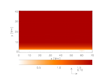
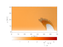
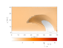
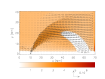
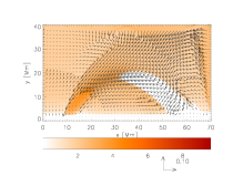
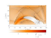
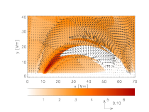
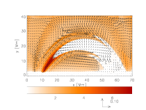
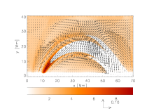
Figure 4: Results of numerical simulation : Temperature (colour maps) and velocity (arrows) profiles at $t=0$ s, $t=100$ s, $t=200$ s, $t=300$ s, $t=400$ s, $t=500$ s, $t=600$ s, $t=700$ s, and $t=800$ s (from top-left to bottom-right). Temperature is drawn in units of $1$ MK. The arrow below each panel represents the length of the velocity vector, expressed in units of $150$ km s^-1.

Fig.4 displays the spatial profiles of plasma temperature (colour maps) and velocity (arrows) resulting from the initial pressure pulse of Eq. (11), which splits into counter-propagating parts. The part which propagates downwards becomes reflected from the dense plasma layers at the photospheric region. This reflected part lags behind the originally upward propagating signal that becomes a slow shock. The applied initial pressure pulse with its amplitude 30 times larger than the same for ambient plasma, was launched at the right foot-point of a loop system. As the plasma is initially pushed upwards, an under-pressure region is created below the initial pulse. This under-pressure region sucks up comparatively less heated plasma, which lags behind the high temperature shock front. As a result, the pressure gradient works against the gravity and forces the material to penetrate into the higher parts of the loop system in form of rarefaction wave. It should be noted that the observed post flare loop systems were not visible initially, and they became visible after filling up of the plasma during the flare process. In the observations, we choose one multi-stranded post flare loop system whose footpoints were separated approximately by 50 Mm, and the width was $\sim$7 Mm. We set our simulated loop system approximately with the same spatial scale of the selected post flare loop system in the observations. In the simulation of internal plasma dynamics of post flare loop system, the snapshot at $t=100$ s will be a reference in which the plasma is lifting up from its one footpoint with the launch of pressure pulse. A similar scenario is also evident in 18:44 UT images of the observations (cf., Figs 2-3). It should also be noted that the cool counterpart of the plasma may be enveloped by its hot counterpart in the simulations similar to the observations. However, initially it may not be realized in the more ideal simulation domain. It is even also difficult to distinguish hot and cool plasma in the observations exactly due to the projection effect as well as dominant coronal emissions in the loop system. However, at $t=400-500$ s, few hot plasma threads are flowing laminar to the cool plasma that may support the observational scenario upto some extent. However, we can not exactly mimic the complex real observational scenario of the presence of multi-temperature plasma in the simulation. At $t=400$ s and later, the slow shock with high temperature front hits at the left footpoint of the loop system and reflects back from the dense plasma near this footpoint. The moving plasma interacts with the reflected shock (cf., t=400-800 s simulation snapshots). Therefore, the moving plasma does not reach exactly at the left footpoint and starts propagating in the opposite direction. This is clearly evident in the simulation, and this scenario matches well with the observations as displayed in the snapshots at 18:58 UT in Figs 2-3. In the simulation, the same scenario became well evident around $t$=800 s when the slow reflected shock interacts with the moving plasma and causes its antipropagation. It should be noted that the moving plasma is also sub-sonic in the numerical simulation that matches well with the observed moving intensity feature.

Due to the interaction of reflected shock and the downward moving plasma , the plasma becomes much compressed near the left foot-point region. Therefore, at this location, the high pressure region does not allow the moving plasma to fall down towards the left foot-point completely due to the gravity. A similar situation is evident in the observations when a mixture of plasma containing both heated and cool material again starts propagating towards the northward footpoint in the post flare loop system (cf., Figs 2-3, 18:57-18:58 UT). In conclusion, although the real observational situation exhibits the complex dynamics of a multi-temperature plasma, our numerical results approximately reproduce the observed post flare plasma dynamics despite our use of a simplified model.

5 Discussions and Conclusion

In the present work, we observe the unique dynamics of cool and hot plasma in a multi-stranded post flare loop system that evolved in the decay phase of a two ribbon M1.0 class flare in AR 11093 on 7 August 2010 using SDO/AIA 304 Å and 171 Å filters. The moving intensity feature and its reflected counterpart are observed in the loop system at multi-temperatures. The observed hot counterpart of the plasma that probably envelopes the cool confined plasma, moves comparatively faster (34 km s^-1) to the later component (29 km s^-1) in form of the spreaded intensity feature. The propagating plasma and intensity reflect from another footpoint of the loop. The subsonic speed of the moving plasma and associated intensity feature may be most likely evolved in the post flare loop system impulsively by the flare heating processes of the loop footpoints.

Recently, Nakariakov & Zimovets (2011) have demonstrated that sub-sonic disturbances propagating along the axis of post flare arcades in two-ribbon flares can be interpreted in terms of slow magnetoacoustic waves. These waves can propagate across the magnetic field, parallel to the magnetic neutral line, because of the wave-guiding effect due to the reflection from the footpoints. Our observed moving intensity feature is also subsonic but propagates along the loop strands rather than along the magnetic neutral line. Using TRACE observations of various flaring events, Li & Zhang (2009b) have statistically studied the dynamics of the propagating brightness features in the post flare loop arcades. They have found that the brightness propagations move with the speeds in the range of 3-39 km s^-1. Our observed speeds of the hot and cool counterparts of the plasma also lie in the same range as observed by Li & Zhang (2009b), which were subsonic motions. They have observed three kind of internal motions in the post flare loop systems, e.g., (i) the excitation of propagating brightness near loop apex that moves towards both the footpoints, (ii) the triggering of perturbation at one end that propagates towards other end, and (iii) multi-spatial excitation and propagation of the brightening in post flare loop systems (PFLs). They have concluded a general 3-D reconnection scenario for the generation of their observed PFL plasma dynamics. They have also found that the propagation of brightness in post flare loops are coupled with the ribbon separation. However, our observed unique moving intensity feature was the propagation of multi-temperature subsonic plasma starting near one footpoint and then its reflection from another footpoint of the post flare loop system. Moreover, in our case, the post flare loop system and the flare ribbons were almost in equilibrium for chosen duration (18:44 UT–18:59 UT) of 15 min. Therefore, we could track the internal plasma dynamics of loop system to compare with the numerical simulation. The two ribbon M1.0 class flare has occurred in a classical way as per the standard reconnection model (e.g, Shiota et al., 2005). The part of filament which was located along the neutral line in between both the ribbons, most likely activated and subsequently reconnected with the overlying coronal field lines that triggered an M1.0 class flare, followed by a long duration post flare phase. However, we observe unique and short duration internal plasma dynamics when the ribbon positions and the post flare loop were almost stable. Therefore, the flare occurred most likely due to standard 3-D multi-stage reconnection event (Shiota et al., 2005), had already subsided for the chosen duration and was not leading much ribbon separation as well as the bulk dynamics of evolved post flare loop systems along these two ribbons. Therefore, we suggest that some local driver generated by impulsive heating due to standard reconnection process leads the observed plasma dynamics in the selected post flare loop system. The reconnection generated impulsive energy deposition by the energetic particles to the ribbons may lead the density as well as pressure perturbations near the loop footpoints. The triggered thermal purturbations may steepen into a slow shock front moving along the loop threads and generates the rarefraction wave behind, which causes the motion of brightened plasma up as observed by SDO/AIA 304 Å and 171 Å filters. The interaction of the hot and cool plasma components with the reflected leading shock causes the antipropagation of multi-temperature plasma and generates the complex dynamics of the loop system as observed by SDO/AIA.

We also attempt a numerical simulation to show a general scenario of an observed post flare plasma dynamics internally in a post flare loop system. However, the real dynamics was excited in more complex plasma and magnetic field conditions in the two-ribbon M1.0 class flaring region in AR 11093 on 7 August 2010. We might not model exactly realistically the way in which the post flare loop system was evolved in the real Sun, and therefore its complex plasma dynamics. In fact, the excitation mechanism could work for some time, it could be located at a different place and it could have a different size, pressure perturbation amplitude and distribution. However, in our simulation we trigger the plasma dynamics by a localized pulse in the pressure that is launched below the transition region. In this way we managed to excite the plasma dynamics which qualitatively mimics on average the observations. The small mismatches like the exact time-scales of the motion of plasma and starting of its reflection etc can be matched by tuning of free parameters in the numerical model.

In conclusion we suggest that the initial thermal pulse launched below the transition region is able to trigger a slow shock manifested mainly as a plasma flow along the loop strands, which is followed by a brightened moving plasma material. This scenario resembles the observed fine structural dynamics of the post flare loop system. We report first time on the observations of a thermal pulse driven multi-temperature plasma in the post flare loop and provide an approximate theoretical explanation of this phenomenon on the basis of numerical simulations we performed. However, further multiwavelength observations should be performed by high-resolution space borne (e.g., SDO, Hinode, STEREO) and complementary ground based observations to shed new light on this kind of unique plasma dynamics. This will also impose a rigid constraint on the stringent simulations of such kind of dynamics in the model solar atmosphere, e.g., the consideration of more realistic atmosphere by taking into account the thermal conduction and radiative cooling effects.

6 Acknowledgments

We thank reviewer for his/her valuable suggestions that improved the manuscript considerably. We acknowledge the use of the SDO/AIA observations for this study. The data is provided curtesy of NASA/SDO, LMSAL, and the AIA, EVE, and HMI science teams. The FLASH code has been developed by the DOE-supported ASC/Alliance Center for Astrophysical Thermonuclear Flashes at the University of Chicago. AKS acknowledges Shobhna Srivastava for the patient encouragement. KM thanks Kamil Murawski for his helps in the visualization of the numerical results.

References

- Andries et al. (2009) Andries, J., van Doorsselaere, T., Roberts, B., Verth, G., Verwichte, E., & Erdélyi, R. 2009, Space Sci. Rev., 149, 3
- Aschwanden (2009) Aschwanden, M. J. 2009, Space Sci. Rev., 149, 31
- Cargill & Priest (1982) Cargill, P. J., & Priest, E. R. 1982, Sol. Phys., 76, 357
- Cheng et al. (2010) Cheng, X., Ding, M. D., Guo, Y., Zhang, J., Jing, J., & Wiegelmann, T. 2010, ApJ, 716, L68
- Fernández et al. (2009) Fernández, C. A., Costa, A., Elaskar, S., & Schulz, W. 2009, MNRAS, 400, 1821
- Harra-Murnion et al. (1998) Harra-Murnion, L. K., et al. 1998, A&A, 337, 911
- Kryshtal & Gerasimenko (2004) Kryshtal, A. N., & Gerasimenko, S. V. 2004, A&A, 420, 1107
- Lee & Deane (2009) Lee, D., & Deane, A. E. 2009, Journal of Computational Physics, 228, 952
- Lemen et al. (2011) Lemen, J. R., Title, A. M., & Akin, D. e. a. 2011, A&A, A8
- Li & Zhang (2009a) Li, L., & Zhang, J. 2009a, ApJ, 703, 877
- Li & Zhang (2009b) Li, L., & Zhang, J. 2009b, ApJ, 690, 347
- Longcope et al. (2009) Longcope, D. W., Guidoni, S. E., & Linton, M. G. 2009, ApJ, 690, L18
- Macnamara & Roberts (2010) Macnamara, C. K., & Roberts, B. 2010, A&A, 515, A41
- Macnamara & Roberts (2011) Macnamara, C. K., & Roberts, B. 2011, A&A, 526, A75
- Nakariakov & Zimovets (2011) Nakariakov, V. M., & Zimovets, I. V. 2011, ApJ, 730, L27
- O’Shea et al. (2007) O’Shea, E., Srivastava, A. K., Doyle, J. G., & Banerjee, D. 2007, A&A, 473, L13
- Reddy et al. (2011) Reddy, V., Ajor Maurya, R., & Ambastha, A. 2011, ArXiv e-prints
- Reeves & Warren (2002) Reeves, K. K., & Warren, H. P. 2002, ApJ, 578, 590
- Shiota et al. (2005) Shiota, D., Isobe, H., Chen, P. F., Yamamoto, T. T., Sakajiri, T., & Shibata, K. 2005, ApJ, 634, 663
- Srivastava (2010) Srivastava, A. K. 2010, Advances in Geosciences, Volume 21: Solar Terrestrial (ST), 21, 315
- Srivastava et al. (2008) Srivastava, A. K., Zaqarashvili, T. V., Uddin, W., Dwivedi, B. N., & Kumar, P. 2008, MNRAS, 388, 1899
- Warren et al. (1999) Warren, H. P., Bookbinder, J. A., Forbes, T. G., Golub, L., Hudson, H. S., Reeves, K., & Warshall, A. 1999, ApJ, 527, L121