Relativistic corrections to the semi-inclusive decay of $\bm{\psi}$ and $\bm{\Upsilon}$

Abstract

In the framework of the nonrelativistic quantum chromodynamics factorization formalism, we study the processes of $\psi(nS)$ and $\Upsilon(nS)$ decay into a lepton pair or a charm pair associated with two jets up to the next-to-leading order in velocity expansion. We present the analytic expressions for the differential decay rate to the invariant mass of the lepton pair or charm pair. We find that the ratio of the next-to-leading order short-distance coefficient to the leading order one is in the range from $-5.5$ to $-12.4$. The relativistic corrections are so large that they modify the leading order prediction significantly. Utilizing the analytic expressions, we also investigate the relativistic corrections in different kinematic regions and their dependence on the masses of the initial-state quarkonium and the final-state fermion. In addition, we study the momentum distribution of $D^{*+}$ in the process $\Upsilon(1S)\to c\bar{c}gg\to D^{*+}X$.

I Introduction

Heavy quarkonium decay phenomena have been extensively studied both in theory and in experiment, from which one gains insight into both the structure of the heavy quarkonium and quantum chromodynamics (QCD) interactions. The predominant annihilation decay modes of the $S$-wave spin-triplet heavy quarkonium are those hadronic decays, radiative decays, and leptonic decays. With abundant data of the $S$-wave spin-triplet heavy quarkonium decays accumulated in experiments, higher order decay processes are also interesting to investigate. Among them, two types of processes are particularly interesting. One type is that the $S$-wave spin-triplet charmonium and bottomonium semi-inclusive decay into a leptonic pair and light hadrons. The other one is the $S$-wave spin-triplet bottomonium semi-inclusive decays into a charm meson pair and light hadrons.

In experiment, charm production via $\Upsilon(1S)$ was studied first by the ARGUS Collaboration Albrecht:1992ap and recently by the BABAR Collaboration :2009wm as well as by the CLEO Collaboration Alex:2010 . BABAR’s results :2009wm provided evidence for an excess of $D^{*\pm}$ production over the expected rate from the virtual photon annihilation process $\Upsilon(1S)\to\gamma^{*}\to c\bar{c}\to D^{*\pm}X$. With a number of $\psi(nS)$ events accumulated at the Beijing Electron Positron Collider (BEPCII) Asner:2008nq and $\Upsilon(nS)$ events accumulated at B factories Brambilla:2004wf , the $S$-wave spin-triplet charmonium and bottomonium semi-inclusive decay into a lepton (charm) pair and light hadrons are expected to be measured well.

In comparison with experimental data, it is necessary to theoretically study those processes precisely. The decay rate of these processes can be analyzed in the framework of nonrelativistic QCD (NRQCD) factorization formalism Bodwin:1994jh . According to it, the decay rates are expressed as a sum of products of short-distance coefficients and NRQCD matrix elements. The short-distance coefficients can be expanded as perturbation series in coupling constant $\alpha_{s}$ at the scale of the heavy quark mass. The long-distance matrix elements can be expressed in a definite way with the typical relative velocity $v$ of the heavy quark in the quarkonium state.

The decay rate of the semi-inclusive leptonic decay process $\psi(\Upsilon)\to l^{+}l^{-}gg$ was first studied by J. P. Leveille and D. M. Scott in the color-singlet model Leveille-Scott:1980 . The polar and azimuthal angular distributions of the lepton pair in this process were also studied in Refs. Korner:1982fn ; Clavelli:1984ru . The semi-inclusive charm decay process $\Upsilon\to c\bar{c}gg$ was first researched in Refs. Fritzsch:1978ey ; Parkhomenko:1994xi , and the invariant mass distribution of $c\bar{c}$ has been studied in Ref. Kang:2007uv . The inclusive charm production in $\Upsilon(nS)$ decay was calculated in Ref. Chung:2008yf . Bigi and Nussinov have taken into account the contribution of $\Upsilon\to c\bar{c}g$ Bigi:1978tj . The exclusive double charmonium production from $\Upsilon$ decay was calculated by Jia Jia:2007hy . The authors of Ref. Zhang:2008pr also considered the $\Upsilon$ decay to two charm jets by including the color-octet contribution. Cheung, Keung, and Yuan calculated the color-octet $J/\psi$ production in the $\Upsilon$ decay Cheung:1996mh .

According to the NRQCD factorization formula, only the leading order (LO) contributions are considered for the processes $\psi(\Upsilon)\to l^{+}l^{-}(c\bar{c})gg$. In the next-to-leading order (NLO), the decay rate receives relativistic corrections, whose long-distance matrix elements are suppressed by $v^{2}$ compared with the LO contribution. Notice that the relativistic corrections to the decay rates in the processes $J/\psi\to\gamma gg$ and $J/\psi\to ggg$ are extremely large and significant Keung:1982jb . One may expect that the decay rates of the processes $\psi(\Upsilon)\to l^{+}l^{-}gg$ and $\Upsilon\to c\bar{c}gg$ also receive considerable contributions from the relativistic corrections since those processes possess similar Feynman diagrams. However, until now, a thorough analysis including the contributions of the NLO NRQCD matrix elements is lacking. In this paper, we analyze the decay rate for $\psi(\Upsilon)\to l^{+}l^{-}(c\bar{c})gg$ up to the NLO in the relativistic expansion in the framework of the NRQCD factorization formula. We calculate the short-distance coefficients of both the LO and the NLO NRQCD matrix elements at the tree level and present the analytic expressions for the distribution of the invariant mass of the lepton pair or the charm pair. With these expressions, we are able to study the relativistic corrections in different kinematic regions, and then provide theoretical discussions. We also investigate the momentum distribution of the charm quark in our work. With convolution of a charm quark fragmenting into a charmed hadron, we are able to predict the momentum distribution of the charmed hadron. Since the treatments for inclusive lepton pair production and charm pair production are quite similar, we concentrate on dealing with the process of $H(^{3}S_{1})\to l^{+}l^{-}gg$. The decay rate of $\Upsilon\to c\bar{c}gg$ is readily obtained by multiplying a color factor and substituting the electromagnetic coupling constant $\alpha$ and the lepton mass $m_{l}$ into the strong coupling constant $\alpha_{s}$ and the charm mass $m_{c}$, respectively.

The remainder of this paper is organized as follows. In Sec. II, we present the NRQCD factorization formula for the differential decay rate of the process $H(^{3}S_{1})\to l^{+}l^{-}gg$ up to the NLO in $v$. In Sec. III, given the notations and kinematic variables used in our calculation, we present the formulas for the differential decay rate as well as the total decay rate. Section IV is devoted to determining the short-distance coefficients corresponding to the LO and the NLO NRQCD matrix elements. In Sec. V, we present the numerical results and provide discussions. A summary is given in Sec. VI.

II NRQCD factorization formula for quarkonium decay process $H(^{3}S_{1})\to l^{+}l^{-}gg$

According to the NRQCD factorization formula, up to relative order $v^{2}$, the differential decay rate for a quarkonium $H$ decay into a lepton pair and light hadrons can be expressed as Bodwin:1994jh

$$d\Gamma[H({}^{3}S_{1})\to l^{+}l^{-}+X]=\frac{dF({}^{3}S_{1})}{m^{2}}\,\langle H|{\mathcal{O}}_{1}({}^{3}S_{1})|H\rangle+\frac{dG({}^{3}S_{1})}{m^{4}}\langle H|{\mathcal{P}}_{1}({}^{3}S_{1})|H\rangle\;,$$ (1)

where $m$ signifies the mass of a heavy quark in $H$, $\langle H|{\mathcal{O}}_{1}({}^{3}S_{1})|H\rangle$ and $\langle H|{\mathcal{P}}_{1}({}^{3}S_{1})|H\rangle$ are the NRQCD matrix elements, and $F({}^{3}S_{1})$ and $G({}^{3}S_{1})$ are the corresponding short-distance coefficients, respectively. Here $H$ can be either charmonium or bottomonium. The four-fermion operators ${\mathcal{O}}_{1}({}^{3}S_{1})$ and ${\mathcal{P}}_{1}({}^{3}S_{1})$ are defined as

$${\mathcal{O}}_{1}({}^{3}S_{1}) = \psi^{\dagger}\bm{\sigma}\chi\cdot\chi^{\dagger}\bm{\sigma}\psi,$$ (2a)

$${\mathcal{P}}_{1}({}^{3}S_{1}) = \frac{1}{2}\left[\psi^{\dagger}\bm{\sigma}\chi\cdot\chi^{\dagger}\bm{\sigma}(-\frac{i}{2}\tensor{\bm{D}})^{2}\psi+\psi^{\dagger}\bm{\sigma}(-\frac{i}{2}\tensor{\bm{D}})^{2}\chi\cdot\chi^{\dagger}\bm{\sigma}\psi\right],$$ (2b)

where $\psi$ and $\chi$ are Pauli spinor fields for annihilating a heavy quark, and creating a heavy antiquark, respectively; $\sigma^{i}$ denotes the Pauli matrix; and $\tensor{\bm{D}}$ is the spatial part of the antisymmetrical covariant derivative: $\psi^{\dagger}\tensor{\bm{D}}\chi\equiv\psi^{\dagger}{\bm{D}}\chi-({\bm{D}}\psi)^{\dagger}\chi$. The subscript 1 on the NRQCD operator indicates that it is a color-singlet operator. According to the velocity-scaling rules given in Ref. Bodwin:1994jh , the matrix element of the operator ${\mathcal{O}}_{1}({}^{3}S_{1})$ in the ${}^{3}S_{1}$ state is of order $v^{3}$ while that of the operator ${\mathcal{P}}_{1}({}^{3}S_{1})$ is of order $v^{5}$. The latter one is suppressed by $v^{2}$, which represents the NLO relativistic corrections to the inclusive $H$ decay.

The vacuum-saturation approximation Bodwin:1994jh can be used to simplify the decay matrix elements in Eq. (2). They read

$$\langle H|{\mathcal{O}}_{1}({}^{3}S_{1})|H\rangle = |\langle 0|\chi^{\dagger}\bm{\sigma}\cdot\bm{\epsilon}^{*}\psi|H\rangle|^{2}\equiv\langle{\mathcal{O}}_{1}\rangle_{H},$$ (3a)

$$\langle H|{\mathcal{P}}_{1}({}^{3}S_{1})|H\rangle = \textrm{Re\,}\big{[}\langle H|\psi^{\dagger}\bm{\sigma}\cdot\bm{\epsilon}\chi|0\rangle\langle 0|\chi^{\dagger}\bm{\sigma}\cdot\bm{\epsilon}^{*}(-\tfrac{i}{2}\tensor{\bm{D}})^{2}\psi|H\rangle\big{]}.$$ (3b)

This approximation is valid up to corrections of relative order $v^{4}$. For convenience, we introduce a dimensionless ratio of the vacuum matrix elements in Eq. (3) for later use Gremm:1997dq ; Bodwin:2006dn :

$$\langle v^{2}\rangle_{H} = \frac{\langle 0|\chi^{\dagger}\bm{\sigma}\cdot\bm{\epsilon}^{*}(-\tfrac{i}{2}\tensor{\bm{D}})^{2}\psi|H\rangle}{{m}^{2}\langle 0|\chi^{\dagger}\bm{\sigma}\cdot\bm{\epsilon}^{*}\psi|H\rangle}.$$ (4)

This quantity characterizes the typical size of relativistic corrections for $H$.

Equation (1) implies that, to predict the decay rate, one needs to determine both the short-distance coefficients and the NRQCD matrix elements. The NRQCD matrix elements have been extensively studied by means of lattice QCD Bodwin:1993wf , the nonrelativistic quark model Eichten:1995 , and fitting the experimental data Bodwin:2007fz ; Guo:2011tz . Therefore, once we determine the short-distance coefficients $F({}^{3}S_{1})$ and $G({}^{3}S_{1})$, with those values of matrix elements, we may calculate the differential decay rate in Eq. (1). To determine the $F({}^{3}S_{1})$ and $G({}^{3}S_{1})$ at the tree level, we apply the factorization formula to the process of an on-shell $Q\bar{Q}$ pair near the threshold in a spin-triplet and color-singlet state decaying to $l^{+}l^{-}gg$:

$$d\Gamma[Q\bar{Q}_{1}({}^{3}S_{1})\to l^{+}l^{-}gg] = \frac{dF({}^{3}S_{1})}{m^{2}}\,\langle Q\bar{Q}_{1}({}^{3}S_{1})|{\mathcal{O}}_{1}({}^{3}S_{1})|Q\bar{Q}_{1}({}^{3}S_{1})\rangle$$ (5)

$$\hbox{}+\frac{dG({}^{3}S_{1})}{m^{4}}\langle Q\bar{Q}_{1}({}^{3}S_{1})|{\mathcal{P}}_{1}({}^{3}S_{1})|Q\bar{Q}_{1}({}^{3}S_{1})\rangle\;.$$

Notice that the factorization formula (5) takes a similar form to (1) except that the hadron state is substituted into the on-shell free quark pair state with the same quantum number as the hadron. The decay rate in (5) can be calculated both in the QCD perturbation theory and in the NRQCD factorization formula. By matching both sides, the short-distance coefficients can then be determined.

III Kinematics and Formulas for the decay rate

III.1 Kinematics and definitions

In this section, we define notations for the kinematics involved in our work. We take $p_{1}$ and $p_{2}$ to be the momenta of the incoming heavy quark $Q$ and heavy antiquark $\bar{Q}$, respectively, which are on their mass shells: $p_{1}^{2}=p_{2}^{2}=m^{2}$. They are expressed as linear combinations of the total momentum $P$ and half of their relative momentum $q$:

$$p_{1} = P/2+q,$$ (6a)

$$p_{2} = P/2-q.$$ (6b)

In the center of mass frame of the quarkonium, the momenta are given by

$$P = (2E,\bm{0}),$$ (7a)

$$q = (0,{\bm{q}}),$$ (7b)

where the orthogonal relation $P\cdot q=0$ is satisfied.

We also assign $k_{1},k_{2}$ to be the momenta of the two final-state gluons, and $l_{1},l_{2}$ to be the momenta of the produced lepton pair. Therefore, the momentum $Q$ of the virtual photon yields to $Q=l_{1}+l_{2}$. These momenta satisfy

$$k_{1}^{2}=k_{2}^{2} = 0,$$ (8a)

$$l_{1}^{2}=l_{2}^{2} = m_{l}^{2},$$ (8b)

where $m_{l}$ denotes the mass of the lepton.

For convenience, we introduce a set of dimensionless variables

$$x_{1} = \frac{2k_{1}\cdot P}{P^{2}},\,\,x_{2}=\frac{2k_{2}\cdot P}{P^{2}},\,\,x_{3}=\frac{2Q\cdot P}{P^{2}},\,\,z=\frac{Q^{2}}{P^{2}},$$ (9a)

$$r = \frac{4m_{l}^{2}}{P^{2}},\,\,\,\,y_{1}=\frac{|{\bm{l}}_{1}|}{|{\bm{l}_{1}}|_{max}}=\frac{|{\bm{l}}_{1}|}{m_{l}}\sqrt{\frac{r}{1-r}},$$ (9b)

where $y_{1}$ represents the momentum fraction for the lepton and $|{\bm{l}_{1}}|_{max}$ denotes the maximum of the lepton momentum in the quarkonium center of mass frame. In the following subsection, we will show that all the involved Lorentz invariant kinematic quantities can be rewritten in terms of these new variables.

III.2 The formulas for the decay rate

III.2.1 Differential decay rate of the invariant mass of the lepton pair

For the decay process $H({}^{3}S_{1})(P)\to l^{+}(l_{1})l^{-}(l_{2})g(k_{1})g(k_{2})$, it involves a four-body phase space integral, which can be expressed as

$$\int\!\!d\phi_{4} = \int\!\!\frac{d^{3}k_{1}}{(2\pi)^{3}2k^{0}_{1}}\frac{d^{3}k_{2}}{(2\pi)^{3}2k^{0}_{2}}\frac{d^{3}l_{1}}{(2\pi)^{3}2l^{0}_{1}}\frac{d^{3}l_{2}}{(2\pi)^{3}2l^{0}_{2}}(2\pi)^{4}\delta^{4}(P-k_{1}-k_{2}-l_{1}-l_{2}).$$ (10)

Since there is no divergence emerging in our calculation, dimensions of the space-time are set to $4$ in (10). In order to compute the invariant mass distribution of the lepton pair, we decompose the four-body phase space integral (10) into the product of a two-body phase space integral for the lepton pair and a three-body one by inserting the following two identities:

$$\int\!\!\frac{d^{4}Q}{(2\pi)^{4}}(2\pi)^{4}\delta^{4}(Q-l_{1}-l_{2})=1,\ \ \ \ \ P^{2}\int\!\!\frac{dz}{2\pi}2\pi\delta(Q^{2}-P^{2}z)=1.$$ (11)

After integrating out the energy $Q^{0}$ through the delta function, we get

$$\int\!\!d\phi_{4} = \int\!\!\frac{dz}{2\pi}\int\!\!d\phi_{3}\int\!\!d\phi_{2},$$ (12)

where $\int\!\!d\phi_{2}$ and $\int\!\!d\phi_{3}$ are expressed as

$$\int\!\!d\phi_{2} = P^{2}\int\!\!\frac{d^{3}l_{1}}{(2\pi)^{3}2l^{0}_{1}}\frac{d^{3}l_{2}}{(2\pi)^{3}2l^{0}_{2}}(2\pi)^{4}\delta^{4}(Q-l_{1}-l_{2}),$$ (13a)

$$\int\!\!d\phi_{3} = \int\!\!\frac{d^{3}Q}{(2\pi)^{3}2Q^{0}}\frac{d^{3}k_{1}}{(2\pi)^{3}2k^{0}_{1}}\frac{d^{3}k_{2}}{(2\pi)^{3}2k^{0}_{2}}(2\pi)^{4}\delta^{4}(P-k_{1}-k_{2}-Q).$$ (13b)

On the other side, the squared amplitude can be expressed as the contraction of the leptonic tensor ${\widetilde{L}}^{\mu\nu}$ and hadronic tensor ${\widetilde{H}}_{\mu\nu}$:

$$|{\mathcal{M}}|^{2}={\widetilde{L}}^{\mu\nu}{\widetilde{H}}_{\mu\nu},$$ (14)

where the leptonic tensor ${\widetilde{L}}^{\mu\nu}$ is given by

$${\widetilde{L}}^{\mu\nu}=\frac{e^{2}}{Q^{4}}{\rm Tr}[(\not\!l_{1}+m_{l})\gamma^{\mu}(\not\!l_{2}-m_{l})\gamma^{\nu}].$$ (15)

It follows after integrating over the phase space momenta that

$$L^{\mu\nu}\equiv\int\!\!d\phi_{2}{\widetilde{L}}^{\mu\nu}=\bigg{(}\!\!-g^{\mu\nu}+\frac{Q^{\mu}Q^{\nu}}{Q^{2}}\bigg{)}\times L,$$ (16)

where the Lorentz invariant $L$ is given by

$$L=\frac{2\alpha}{3z}\ \sqrt{1-\frac{r}{z}}\ (1+\frac{r}{{2z}}),$$ (17)

where $\alpha$ is the fine structure constant. As a result, we are able to write the decay rate as

$$\Gamma=\frac{1}{2}\int\!\!\frac{dz}{2\pi}L\int\!\!d\phi_{3}{\widetilde{H}}_{\mu\nu}\bigg{(}-g^{\mu\nu}+\frac{Q^{\mu}Q^{\nu}}{Q^{2}}\bigg{)},$$ (18)

where the factor $\frac{1}{2}$ accounts for the indistinguishability of the two gluons in the final states. It is not hard to find that the second term in the parentheses of (18) does not contribute due to the current conservation.

The three-body phase space integral $\int\!\!d\phi_{3}$ can generically be expressed as the integral of two dimensionless variables $x_{1}$ and $x_{2}$:

$$\int\!\!d\phi_{3} = \frac{P^{2}}{128\pi^{3}}\int\!\!dx_{1}dx_{2}.$$ (19)

Up to now, we have reduced the four-body phase space integral (10) into the integration over three variables: $z$, $x_{1}$, and $x_{2}$. The corresponding boundaries for these variables are given by

$$\frac{1-x_{1}-z}{1-x_{1}}\geq x_{2}\geq 1-x_{1}-z,\ \ \ 1-z\geq x_{1}\geq 0,\ \ \ 1\geq z\geq r.$$ (20)

To simplify further the calculation, we make the variable transformation:

$$x_{1} = (1-z)x,$$ (21a)

$$x_{2} = \frac{(1-z)(1-x)[1-(1-z)xy]}{1-(1-z)x}.$$ (21b)

After this transformation, the area of the integration is significantly simplified as

$$1\geq x\geq 0,\,\,\,\,\,\,\,\,\,\,\,\,\,1\geq y\geq 0.$$ (22)

Now, the expression of the decay rate reduces to

$$\Gamma=\frac{1}{2}\frac{P^{2}}{(4\pi)^{4}}\int^{1}_{r}dz\int^{1}_{0}dx\int^{1}_{0}dy\frac{(1-z)^{3}(1-x)x}{1-(1-z)x}L\times(-g^{\mu\nu}){\widetilde{H}}_{\mu\nu}.$$ (23)

From (23), we notice the principal task is to analyze the subprocess $H(^{3}S_{1})\to\gamma^{*}gg$ (corresponding to the contribution from the hadron part ${\widetilde{H}}_{\mu\nu}g^{\mu\nu}$). In the next section, we will use Eq. (23) to evaluate the total decay rate as well as the differential decay rate over the invariant mass of the lepton pair, equivalently, the dimensionless variable $z$.

III.2.2 Momentum distributions of the charm quark and the charmed hadron

In this section, we first derive the formulas to calculate the momentum distribution of the charm quark in the decay process $\Upsilon\to g^{*}gg\to c\bar{c}gg$. The momentum distribution of a charmed hadron $h$ is then obtained by convolving it with a fragmentation function, which describes a charm quark fragmentation into the meson $h$.

As introduced in Sec. III.2.1, we decompose the phase space integration into two parts by inserting the identities (11). Since we want to observe the momentum distribution of the charm quark, we can integrate out the momenta of the two final-state gluons. To this end, we introduce a tensor $T^{\mu\nu}$ which depends only on the momenta $P$ and $Q$ as

$$T^{\mu\nu} \equiv \int\!\!{d^{3}k_{1}\over(2\pi)^{3}2k^{0}_{1}}{d^{3}k_{2}\over(2\pi)^{3}2k^{0}_{2}}(2\pi)^{4}\delta^{4}(P-Q-k_{1}-k_{2}){\widetilde{H}}^{\mu\nu}$$ (24)

$$= (-g^{\mu\nu}+\frac{Q^{\mu}Q^{\nu}}{Q^{2}})H_{1}+\frac{1}{P^{2}}(P^{\mu}-Q^{\mu}\frac{P\cdot Q}{Q^{2}})(P^{\nu}-Q^{\nu}\frac{P\cdot Q}{Q^{2}})H_{2},$$

where $H_{1}$, $H_{2}$ are Lorentz invariant form factors. In the last step of (24), we have applied the Lorentz covariance and current conservation. By contracting $g^{\mu\nu}$ and $P^{\mu}P^{\nu}$ separately in (24), we are able to obtain the expressions of these two form factors. We notice that $H_{1}$ and $H_{2}$ are independent on the momenta of the two final fermions. To obtain the decay rate, we need to include the charm quark pair part as well as the remaining phase space.

Contracting with the leptonic tensor, we readily obtain

$${\widetilde{T}} \equiv T^{\mu\nu}{\widetilde{L}}_{\mu\nu}=\int\!\!{d^{3}k_{1}\over(2\pi)^{3}2k^{0}_{1}}{d^{3}k_{2}\over(2\pi)^{3}2k^{0}_{2}}(2\pi)^{4}\delta^{4}(P-Q-k_{1}-k_{2})\times\frac{2\pi r}{m_{l}^{2}}\times T$$ (25)

$$= \frac{2\pi r\alpha}{m_{l}^{2}z^{2}}\bigg{\{}(r+2z)H_{1}-H_{2}\bigg{[}(1-r)y_{1}^{2}+r+z-x_{3}\sqrt{(1-r)y_{1}^{2}+r}\bigg{]}\bigg{\}}.$$

Now, we turn to carry out the two phase space integration $\int\!\!d\phi_{2}$ and $\int\!\!d\phi_{3}$. For $\int\!\!d\phi_{2}$, we have

$$\int\!\!\!d\phi_{2} = P^{2}\int\!\!{d^{3}l_{1}\over(2\pi)^{3}2l^{0}_{1}}{d^{3}l_{2}\over(2\pi)^{3}2l^{0}_{2}}(2\pi)^{4}\delta^{4}(l_{1}+l_{2}-Q)$$ (26)

$$= \frac{P^{2}}{8\pi}\int\!\!\frac{|{\bm{l}}_{1}|d|{\bm{l}}_{1}|}{\sqrt{{\bm{l}}_{1}^{2}+m_{c}^{2}}|\bm{Q}|}$$

$$= \frac{m_{l}^{2}}{2\pi r}\int\!\!\frac{y_{1}dy_{1}}{\sqrt{(1-r)y_{1}^{2}+r}\sqrt{x_{3}^{2}-4z}},$$

with the boundaries of $y_{1}$:

$$y_{1+}\geq y_{1}\geq|y_{1-}|,$$ (27)

where

$$y_{1\pm}=\frac{x_{3}}{2\sqrt{1-r}}\bigg{(}\sqrt{1-\frac{4z}{x_{3}^{2}}}\pm\sqrt{1-\frac{r}{z}}\bigg{)}.$$ (28)

We then deal with the phase space integral $\int\!\!d\phi_{3}$. Analogously, we can reduce the integral $\int\!\!d\phi_{3}$ into (19). Nevertheless, since the boundaries (28) contain $x_{3}$, we prefer to choose another set of integration variables, such as $x_{1}$ and $x_{3}$:

$$\int\!\!d\phi_{3} = {P^{2}\over 128\pi^{3}}\int\!\!dx_{3}dx_{1}.$$ (29)

The corresponding boundaries of $x_{3}$ and $x_{1}$ are

$$1+z\geq x_{3}\geq 2\sqrt{z},$$ (30a)

$$x_{1+}\geq x_{1}\geq x_{1-},$$ (30b)

where

$$x_{1\pm}=\frac{1}{2}\bigg{(}2-x_{3}\pm\sqrt{x_{3}^{2}-4z}\bigg{)}.$$ (31)

In addition, as shown in (12), to get the decay rate, we should include another integration over $z$. The corresponding boundaries of $z$ are shown in (20) to be $1\geq z\geq r$.

Finally, the decay rate can be expressed as

$$\Gamma=\frac{1}{2}\frac{P^{2}}{(4\pi)^{4}}\int\!\!dzdx_{3}dx_{1}dy_{1}\frac{y_{1}}{\sqrt{(1-r)y_{1}^{2}+r}\sqrt{x_{3}^{2}-4z}}\times T,$$ (32)

where $T$ is defined in (25).

In order to get the momentum distribution, we need to change the integration order in (32), and to make $y_{1}$ be the last integral. Notice that the boundaries of $y_{1}$ are independent of $x_{1}$; we need not change the order of the integration of $x_{1}$. This calculation is tedious but straightforward. Here we present the expression as follows:

$$\Gamma = \frac{1}{2}\frac{P^{2}}{2(4\pi)^{5}}\bigg{(}\int_{0}^{\frac{\sqrt{1-r}}{2}}\!\!dy_{1}\int_{r}^{z_{-}}\!\!dz\int_{x^{\prime}_{3-}}^{x^{\prime}_{3+}}\!\!dx_{3}+\int_{0}^{1}\!\!dy_{1}\int_{z_{-}}^{z_{+}}\!\!dz\int_{x^{\prime}_{3-}}^{1+z}\!\!dx_{3}\bigg{)}\int_{x_{1-}}^{x_{1+}}dx_{1}$$ (33)

$$\times\frac{y_{1}}{\sqrt{(1-r)y_{1}^{2}+r}\sqrt{x_{3}^{2}-4z}}\times T,$$

where the boundaries of $x_{1}$ are given in (31), and

$$x^{\prime}_{3\pm}=\frac{2}{r}\bigg{(}z\sqrt{(1-r)y_{1}^{2}+r}\pm y_{1}\sqrt{(1-r)(z-r)z}\bigg{)}.$$ (34)

In addition, the boundaries of variable $z$ are the positive solution of the following equation:

$$\frac{(1+z_{\pm})\sqrt{1-\frac{r}{z_{\pm}}}\mp(1-z_{\pm})}{2\sqrt{1-r}}=y_{1}.$$ (35)

With the formula (33), and the boundaries (31) (34) (35), we can carry out a calculation of the distribution of the charm quark momentum fraction $y_{1}$. Now, we go further to investigate the charmed-hadron momentum distribution. As discussed in Ref. Bodwin:2007fz , the momentum distribution of a charmed hadron produced in $\Upsilon$ decay is softer than that of the charm, due to the effect of hadronization. The momentum distribution of a charmed hadron $h$ can be obtained by convolving the charm momentum distribution with a fragmentation function for the charm quark fragmentation into the $h$.

The fragmentation function $D_{c\to h}(z^{\prime})$ describes the probability of a charm quark with light-cone momentum $l_{1}^{0}+|{\bm{l}_{1}}|$ hadronizing into a charmed hadron $h$ with light-cone momentum $l^{0}_{h}+|{\bm{l}_{h}}|=z^{\prime}(l_{1}^{0}+|{\bm{l}_{1}}|)$. The fraction $z^{\prime}$ can be expressed in terms of scaled light-cone momentum fractions $z_{1}$ for the charm and $z_{h}$ for the charmed hadron, which are analogous to the scaled momenta $y_{1}$ and $y_{h}$ Bodwin:2007zf , where $z_{1}$ is

$$z_{1}=\frac{\sqrt{(1-r)y_{1}^{2}+r}+\sqrt{1-r}\,y_{1}}{1+\sqrt{1-r}}.$$ (36)

Then, the fraction $z^{\prime}$ is expressed as

$$z^{\prime}=\frac{z_{h}}{z_{1}}\times\frac{\left.(l^{0}_{h}+|{\bm{l}_{h}}|)\right|_{\textrm{max}}}{\left.(l^{0}_{1}+|{\bm{l}_{1}}|)\right|_{\textrm{max}}},$$ (37)

where the last factor on the right-hand side of Eq. (37) becomes unity if the difference between the mass of the charm quark and that of the charmed hadron can be neglected. With this approximation, the momentum distribution of the charmed hadron can be written as Bodwin:2007fz

$$\frac{d\Gamma}{dy_{h}} = \frac{dz_{h}}{dy_{h}}\int_{z_{h}}^{z_{m}}\frac{dz_{1}}{z_{1}}\,D_{c\to h}(z_{h}/z_{1})\,\frac{dy_{1}}{dz_{1}}\frac{d\Gamma}{dy_{1}}$$ (38)

$$= \frac{\sqrt{1-r}}{\sqrt{(1-r)y_{h}^{2}+r}}\int_{y_{h}}^{y_{m}}dy_{1}\mathcal{D}_{c\to h}\left(\frac{\sqrt{(1-r)y_{h}^{2}+r}+\sqrt{1-r}y_{h}}{\sqrt{(1-r)y_{1}^{2}+r}+\sqrt{1-r}y_{1}}\right)\frac{d\Gamma}{dy_{1}},$$

where $\mathcal{D}_{c\to h}(z^{\prime})=z^{\prime}D_{c\to h}(z^{\prime})$, $y_{m}$ represents the upper boundary for $y_{1}$ in (33), which equals $\sqrt{1-r}/2$ and 1 corresponding to the first term and the second term in the parentheses, and $z_{m}$ corresponds to the value of $z_{1}$ when $y_{1}$ takes $y_{m}$ in (36).

The formulas (33) (38), and the boundaries (31) (34) (35) can be used to carry out a calculation of the distribution of the charmed-hadron momentum fraction $y_{h}$. In Sec. V, we will utilize these formulas to make predictions.

IV Matching the short-distance coefficients up to NLO in $v$

In this section, we determine the differential short-distance coefficients $dF(^{3}S_{1})$ and $dG(^{3}S_{1})$ that appeared in (1). The short-distance coefficients are then readily obtained by integrating over the integration variables. Now, we describe the strategy. By employing the formulas derived in the previous section, we first calculate the differential decay rate for the process of a color-singlet spin-triplet $S$-wave heavy quark pair decay into a lepton pair plus two gluons $Q{\bar{Q}}_{1}(^{3}S_{1})\to l^{+}l^{-}gg$ in the QCD perturbation theory, up to the NLO in $v$, and then carry out the differential decay rate of the same process in the NRQCD factorization formula. Finally, the short-distance coefficients $dF(^{3}S_{1})$ and $dG(^{3}S_{1})$ in (1) are immediately determined by identifying these two calculations.

IV.1 Amplitude of $Q\bar{Q}\to\gamma^{*}gg$

As we have demonstrated in (17) (23) (25), and (33), the lepton part has been explicitly written out. We still have to deal with the subprocess $Q(p_{1})\bar{Q}(p_{2})\to\gamma^{*}(Q)g(k_{1})g(k_{2})$. At the tree level, there are 6 diagrams contributing to the amplitude as shown in Fig. 1. Given the momenta defined in Sec. III.1, the amplitude of the process reads

$$A(s_{1},s_{2})\;=\;\bar{v}(p_{2},s_{2})\;T_{\mu}\;u(p_{1},s_{1}),$$ (39)

where $u(p_{1},s_{1})$ and $v(p_{2},s_{2})$ are the spinors of the heavy quark and antiquark, respectively, and $T_{\mu}$ represents the products of Dirac matrices and color-space matrices. According to Fig. 1, the expression of $T_{\mu}$ reads

$$T_{\mu} = (-ie_{Q}eg_{s}^{2})\ T^{b}T^{a}\otimes\not\!\epsilon_{2}^{*}(k_{2})\frac{1}{{\not\!k_{2}-\not\!p_{2}-m}}\not\!\epsilon_{1}^{*}(k_{1})\frac{1}{{\not\!k_{1}+\not\!k_{2}-\not\!p_{2}-m}}\gamma_{\mu}+5\ \textrm{perms},$$ (40)

where $e,g_{s}$ denote the QED and QCD coupling constant, respectively, $e_{Q}$ denotes the electric charge number of the heavy quark, $a,\epsilon_{1}$ and $b,\epsilon_{2}$ represent the color indices and the polarization vectors of the two gluons, and $\mu$ corresponds to the Lorentz index of the virtual photon.

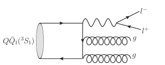
Figure 1: The tree-level Feynman diagrams for $Q\bar{Q}_{1}({}^{3}S_{1})\to l^{+}l^{-}gg$. For simplicity, the crossed diagrams have been suppressed.

IV.2 Projection of spin-triplet $Q\bar{Q}$ state

The amplitude given in (39) describes the decay of the heavy quark and the antiquark state with the spins of the third component $s_{1}$ and $s_{2}$, respectively. To calculate the decay of the $Q\bar{Q}$ in the spin-triplet state and color-singlet state, one needs to project the total spin state of the $Q\bar{Q}$ pair onto the spin-triplet and color-singlet $Q(p_{1})\bar{Q}(p_{2})$ state. This can be done by introducing the projection operator $\Pi_{3}(p_{1},p_{2})$Bodwin:2002hg expressed by

$$\Pi_{3}(p_{1},p_{2}) = \sum_{s_{1},s_{2}}u(p_{1},s_{1})\bar{v}(p_{2},s_{2})\langle\frac{1}{2},s_{1};\frac{1}{2},s_{2}|1\epsilon\rangle\otimes\frac{\mathbf{1}_{c}}{\sqrt{N_{c}}}$$ (41)

$$= -\frac{1}{8\sqrt{2}E^{2}(E+m)}(/\!\!\!{p_{1}}+m)(\,/\!\!\!P\!+\!2E)\,/\!\!\!\epsilon(/\!\!\!p_{2}-m)\otimes\frac{\mathbf{1}_{c}}{\sqrt{N_{c}}},$$

where $\mathbf{1}_{c}$ is the unit matrix in the fundamental representation of the color SU(3) group, and $\epsilon$ is the polarization vector of the spin-triplet state. The above spin-triplet projector is derived by assuming the nonrelativistic normalization convention for Dirac spinor. With this projection operator, the amplitude for a spin-triplet and color-singlet $Q\bar{Q}$ pair annihilation decay reads

$${\mathcal{A}}_{\mu}^{\rm sing}[Q\bar{Q}\to\gamma^{*}gg]=\textrm{Tr}\bigg{\{}\Pi_{3}(p_{1},p_{2})T_{\mu}\bigg{\}},$$ (42)

where the trace is understood to act on both Dirac and color spaces.

IV.3 Projection of $S$-wave amplitude

Besides projecting the $Q\bar{Q}$ pair onto the spin-triplet state, to account for the contribution from the $S$-wave orbital-angular-momentum state, one has to project further the $Q\bar{Q}$ state onto the $S$-wave state. It can be done by averaging the amplitude ${\mathcal{A}}^{\rm sing}$ over all directions of the relative momentum $\mathbf{q}$ in the $Q\bar{Q}$ rest frame.

The amplitude can be expanded in terms of the powers of ${\bm{q}}^{2}$ and the series can be truncated to the desired order. Since here we are only interested in the NLO relativistic corrections, we may do it by expanding the spin-triplet amplitude ${\mathcal{A}}^{\rm sing}$ in $q^{\mu}$ through quadratic order, then making the following replacement Bodwin-Lee:2003 :

$$q^{\mu}q^{\nu} \to \frac{\mathbf{q}^{2}}{3}\>\Pi^{\mu\nu}(P),$$ (43)

where

$$\Pi^{\mu\nu}(P) \equiv -g^{\mu\nu}+\frac{P^{\mu}P^{\nu}}{P^{2}}.$$ (44)

IV.4 The decay rate of $Q\bar{Q}_{1}({{}^{3}S_{1}})\to l^{+}l^{-}gg$ up to relative order $v^{2}$

Since the calculation for the momentum distributions of the charm quark and charmed hadron are similar to that of the invariant mass distribution of the lepton pair, in the following subsections, we merely demonstrate the latter.

We now proceed to compute the lepton pair invariant mass distribution for the process $Q\bar{Q}_{1}({}^{3}S_{1})\to l^{+}l^{-}gg$ at the LO and the NLO in $v$, based on the techniques described in Sec. IV.3.

We first expand the amplitude given in (42) in terms of ${\bm{q}}$ up to quadratic order, then apply (43) to extract the $S$-wave part

$${\overline{A}}_{\mu}={\overline{A}}^{(0)}_{\mu}+{\overline{A}}_{\mu}^{(2)}\frac{{\bm{q}}^{2}}{m^{2}}+{\mathcal{O}}({\bm{q}}^{4}).$$ (45)

The hadronic tensor in (23) is then given by squaring the amplitude ${\overline{A}}_{\mu}$, averaging over the polarizations of the initial state, and summing over the polarizations of the two gluons:

$${\widetilde{H}}_{\mu\nu}=\frac{1}{3}\sum_{\rm{pol}}{\overline{A}}_{\mu}{\overline{A}}^{*}_{\nu}.$$ (46)

Substituting it into (23), the decay rate is expressed as

$$\Gamma = -\frac{4E^{2}}{2(4\pi)^{4}}\int\!\!dzdxdy\frac{(1-z)^{3}(1-x)x}{1-(1-z)x}\times L\times\frac{1}{3}\sum_{pol}{\overline{A}}^{\mu}{\overline{A}}^{*}_{\mu}$$ (47)

$$= -\frac{2m^{2}}{3}\frac{1}{(4\pi)^{4}}\int\!\!dzdxdy\frac{(1-z)^{3}(1-x)x}{1-(1-z)x}\times L$$

$$\times\sum_{pol}\bigg{[}{\overline{A}}^{(0)\mu}{\overline{A}}^{(0)*}_{\mu}+\bigg{(}{\overline{A}}^{(0)\mu}{\overline{A}}^{(0)*}_{\mu}+2{\textrm{R}e}[{\overline{A}}^{(0)\mu}{\overline{A}}^{(2)*}_{\mu}]\bigg{)}\times\frac{{\bm{q}}^{2}}{m^{2}}+{\mathcal{O}}({\bm{q}}^{4})\bigg{]}\;.$$

In the calculation, we employ the mathematica package Feyncalc Mertig:1990an to implement the arithmetic of Dirac trace and Lorentz contraction. The resultant distribution of the invariant mass of the lepton pair reads

$$\frac{d\Gamma}{dz} = \frac{4\alpha^{2}\alpha_{s}^{2}e_{Q}^{2}}{27\pi m^{2}}\sqrt{1-\frac{r}{z}}\ (1+\frac{r}{2z})\;\bigg{(}f_{0}(z)+f_{2}(z)\frac{{\bm{q}}^{2}}{m^{2}}\bigg{)},$$ (48)

where the analytic expressions for $f_{0}(z)$ and $f_{2}(z)$ are given by

$$f_{0}(z) = \frac{4}{z(1-z)^{2}}\bigg{\{}\bigg{[}(2z^{3}-z^{2}-12z+8)\tan^{-1}\bigg{(}\sqrt{\frac{1-z}{z}}\bigg{)}+2\sqrt{z(1-z)}(4z^{2}-9z+8)\bigg{]}$$ (49)

$$\times \tan^{-1}\bigg{(}\sqrt{\frac{1-z}{z}}\bigg{)}-9(1-z)(z^{2}-2z+2)+z(5z^{2}-14z+3)\log z\bigg{\}},$$

and

$$f_{2}(z) = \frac{4}{9z(1-z)^{3}}\bigg{\{}\bigg{[}3(4z^{4}-8z^{3}-57z^{2}+96z-38)\tan^{-1}\left(\sqrt{\frac{1-z}{z}}\right)-6\sqrt{z(1-z)}$$ (50)

$$\times (17z^{2}-51z+31)\bigg{]}\tan^{-1}\left(\sqrt{\frac{1-z}{z}}\right)-(1-z)(61z^{3}-192z^{2}+386z-198)$$

$$+ 2z(z^{3}-55z^{2}+43z-13)\log z\bigg{\}}.$$

Notice that, when extracting the relativistic corrections, we do not expand $r$ in terms of $E=\sqrt{m^{2}+{\bm{q}}^{2}}$ in (48). Actually, from the expression of (48), we find the differential decay rate is sensitive to the value of $r$ in the region of $z\to r$. Moreover, the decay rate develops a strong dependence on $r$ from this region, i.e., $\int_{r}dz\frac{d\Gamma}{dz}\propto\log r$. In our numerical calculation, we will choose $r=4m_{l}^{2}/P^{2}=4m_{l}^{2}/m_{H}^{2}$, where $m_{H}$ is the mass of the initial quarkonium. Since the quarkonium mass is well measured, this choice may also reduce the uncertainties from the input parameters.

For the same reasons, we will make the choice of $r=4m_{D}^{2}/m_{H}^{2}$ in (33) when evaluating the momentum distributions for the charm quark and the charmed hadron.

IV.5 The short-distance coefficients $d\bm{F({}^{3}S_{1})}$ and $d\bm{G({}^{3}S_{1})}$

To determine the short-distance coefficients, we need to calculate the parton level process $Q\bar{Q}_{1}({}^{3}S_{1})\to l^{+}l^{-}gg$ in the NRQCD factorization formula. The involved matrix elements are easily obtained by perturbative NRQCD:

$$\langle Q\bar{Q}_{1}({}^{3}S_{1})|{\mathcal{O}}_{1}(^{3}S_{1})|Q\bar{Q}_{1}({}^{3}S_{1})\rangle = 2N_{c},$$ (51a)

$$\langle Q\bar{Q}_{1}({}^{3}S_{1})|{\mathcal{P}}_{1}(^{3}S_{1})|Q\bar{Q}_{1}({}^{3}S_{1})\rangle = 2N_{c}\,\bm{q}^{2},$$ (51b)

where the state of the heavy quark pair is normalized nonrelativistically, and the factor $2N_{c}$ accounts for the spin and color normalization.

Substituting (51) into (5), we can write down the corresponding differential decay rate in the NRQCD factorization formula:

$$\frac{d}{dz}\Gamma(Q\bar{Q}_{1}({}^{3}S_{1})\to l^{+}l^{-}gg)=\frac{2N_{c}}{m^{2}}\bigg{(}\frac{d\,F({}^{3}S_{1})}{dz}+\frac{d\,G({}^{3}S_{1})}{dz}\frac{{\bm{q}}^{2}}{m^{2}}+{\mathcal{O}}({\bm{q}}^{4})\bigg{)}.$$ (52)

Matching the QCD side and the NRQCD side by equating (48) with (52), one determines the short-distance coefficients $\frac{d\,F({}^{3}S_{1})}{dz}$ and $\frac{d\,G({}^{3}S_{1})}{dz}$:

$$\frac{d\,F({}^{3}S_{1})}{dz} = \frac{2\alpha^{2}\alpha_{s}^{2}e_{Q}^{2}}{81\pi}f_{0}(z)\sqrt{1-\frac{r}{z}}\ (1+\frac{r}{2z}),$$ (53a)

$$\frac{d\,G({}^{3}S_{1})}{dz} = \frac{2\alpha^{2}\alpha_{s}^{2}e_{Q}^{2}}{81\pi}f_{2}(z)\sqrt{1-\frac{r}{z}}\ (1+\frac{r}{2z}).$$ (53b)

Employing (53), we are able to provide the following discussions. It is instructive to look at the ratio

$$t(z)\equiv\frac{d\,G({}^{3}S_{1})}{dz}/\frac{d\,F({}^{3}S_{1})}{dz}=\frac{f_{2}(z)}{f_{0}(z)},$$ (54)

which solely depends on variable $z$. This ratio characterizes the importance of the NLO relativistic corrections compared to the LO contribution. To visualize the relation, we plot the ratio $t(z)$ over the variable $z$ in Fig. 2.

Figure 2: Distribution of the scaled variable $z$ for the invariant mass of the lepton pair. We use $F,G$ to signify the short-distance coefficients $F({}^{3}S_{1})$ and $G({}^{3}S_{1})$.

From this figure, we see that the ratio $t(z)$ is negative in the physical region with the variable $z$ ranging from 0 to 1. We also notice that the magnitude of $t(z)$ rises rapidly with the increase of $z$.

In addition, we go further to analyze the two limits of the ratio $t(z)$. In the limit of $z\to 0$, there is

$$\lim_{z\to 0}t(z) = \frac{132-19\pi^{2}}{12(\pi^{2}-9)}=-5.32\,,$$ (55)

which agrees with the ratio of the short-distance coefficient of the NLO relativistic corrections and that of the LO for the processes $\psi\to\gamma gg$ and $\psi\to ggg$, as expected. In the limit of $z\to 1$, it follows from Eqs. (49) and (50) that $f_{0}(z)\to 0$, and $f_{2}(z)\to{\rm const}$. As a consequence,

$$\lim_{z\to 1}t(z) = -\,\frac{8}{1-z}+\frac{4}{3}+{\mathcal{O}}(1-z)\,.$$ (56)

From (56), we see that the ratio $t(z)$ goes to infinity in the limit of $z\to 1$, which is the result of a vanishing $f_{0}(z)$ in that limit. In fact, we can see that $f_{0}(z)$ vanishes in the limit of $z\to 1$ from amplitude. When the momenta of two real gluons are soft, the amplitude of $J/\psi\to\gamma^{*}gg$ can be separated into

$${\mathcal{A}}(J/\psi\to\gamma^{*}gg) = g_{s}^{2}\bigg{(}\frac{p_{1}\cdot\epsilon_{1}p_{1}\cdot\epsilon_{2}}{p_{1}\cdot k_{1}p_{1}\cdot k_{2}}+\frac{p_{2}\cdot\epsilon_{1}p_{2}\cdot\epsilon_{2}}{p_{2}\cdot k_{1}p_{2}\cdot k_{2}}-\frac{p_{1}\cdot\epsilon_{1}p_{2}\cdot\epsilon_{2}+p_{2}\cdot\epsilon_{1}p_{1}\cdot\epsilon_{2}}{p_{1}\cdot k_{1}p_{2}\cdot k_{2}}\bigg{)}$$ (57)

$$\times\frac{\delta^{a_{1}a_{2}}}{2}{\mathcal{A}}(J/\psi\to\gamma^{*}),$$

where $\epsilon_{i}$ and $a_{i}$ indicate the polarization vector and color index of the $i$ gluon. At LO in $v$, there is $p_{1}=p_{2}=\tfrac{P}{2}$, and therefore ${\mathcal{A}}(J/\psi\to\gamma^{*}gg)$ vanishes. Consequently, $f_{0}(z)$ vanishes in $z\to 1$.

Figure 2 and Eq. (55) combine to indicate that the NLO relativistic corrections in this process are not only large but increase rapidly with the rise of the virtuality of the intermediate photon. One may doubt the convergence of the expansion series in $v$. In Ref. Bodwin:2002hg , the authors calculated the relativistic corrections to the decay rate of $\Upsilon\to ggg$ up to $v^{4}$. Their results indicate the relativistic corrections from the color-singlet matrix elements are convergent. Since the Feynman graphs are quite similar, we expect the relativistic expansion will be convergent in the process of $\Upsilon\to l^{+}l^{-}gg$.

The short-distance coefficients $G({}^{3}S_{1})$ and $F({}^{3}S_{1})$ can be readily obtained by integrating out the variable $z$. Finally, substituting the short-distance coefficients given in Eqs. (53) into Eq. (1), we present the differential decay rates in the NRQCD factorization formula for the process $H(^{3}S_{1})\to l^{+}l^{-}gg$:

$$\frac{d\Gamma[H(^{3}S_{1})\to l^{+}l^{-}gg]}{dz} = \bigg{(}\frac{dF({}^{3}S_{1})}{dz}+\frac{dG({}^{3}S_{1})}{dz}\langle{v^{2}}\rangle_{H}\bigg{)}\frac{\langle{\mathcal{O}}\rangle_{H}}{m^{2}},$$ (58)

where the matrix element $\langle{v^{2}}\rangle_{H}$ is previously defined in (4). The decay rate is correspondingly achieved by integrating out the variable $z$.

The differential short-distance coefficients as well as the decay rate for the lepton pair production can be easily extended to the process $\Upsilon(nS)\to c\bar{c}gg$, where the charm pair is produced through one virtual gluon instead of the virtual photon. One can get them by multiplying a color factor 5/24, and substituting $m_{l}$ and $e_{Q}^{2}\alpha^{2}$ into $m_{D}$ and $\alpha_{s}^{2}$ on the right-hand side of (53) and (58).

V Numerical Results and discussions

In this section, we first numerically evaluate the total decay rate and the short-distance coefficients for various processes, and then discuss the momentum distribution related to the charmed meson $D^{*+}$ in the process $\Upsilon(1S)\to c\bar{c}gg\to D^{*+}X$.

V.1 Decay rate and the short-distance coefficients

In this subsection, we employ the obtained differential short-distance coefficients (53) and the decay rate (58) to make numerical predictions for the decay rate of the processes $H(^{3}S_{1})\to l^{+}l^{-}(c\bar{c})gg$. The corresponding discussions are also presented.

Table 1: Numerical values for the parameters of different initial-state particles: the mass $m_{H}$, strong coupling constant $\alpha_{s}(m_{H}/2)$, the NRQCD matrix elements $\langle{\mathcal{O}}_{1}\rangle_{H}$ and the value of $\langle v^{2}\rangle_{H}$.

		$m_{H}(\rm GeV)$		$\alpha_{s}(m_{H}/2)$		$\langle{\mathcal{O}}_{1}\rangle_{H}(\rm GeV^{3})$		$\langle v^{2}\rangle_{H}$
$J/\psi$		3.097		0.334		0.440		0.225
$\psi(2S)$		3.686		0.300		0.274		0.633
$\Upsilon(1S)$		9.460		0.215		3.07		0.057
$\Upsilon(2S)$		10.023		0.211		1.62		0.179
$\Upsilon(3S)$		10.355		0.210		1.28		0.251

Table 2: The ratio $r$, theoretical predictions for the decay rate, the ratio between the NLO rate and LO rate, and the ratio between the short-distance coefficients.

		$r$		$\Gamma^{(0)}(\rm keV)$		$\Gamma^{(2)}(\rm keV)$		$\Gamma^{(2)}/\Gamma^{(0)}$		$G_{1}({}^{3}S_{1})/{F_{1}({}^{3}S_{1})}$
$J/\psi\to e^{+}e^{-}gg$		$1.08\times 10^{-7}$		$4.73\times 10^{-1}$		$-5.91\times 10^{-1}$		$-125\%$		-5.56
$J/\psi\to\mu^{+}\mu^{-}gg$		$4.69\times 10^{-3}$		$1.08\times 10^{-1}$		$-1.57\times 10^{-1}$		$-145\%$		-6.49
$\psi(2S)\to e^{+}e^{-}gg$		$7.66\times 10^{-8}$		$2.43\times 10^{-1}$		$-8.56\times 10^{-1}$		$-352\%$		-5.55
$\psi(2S)\to\mu^{+}\mu^{-}gg$		$3.31\times 10^{-3}$		$5.98\times 10^{-2}$		$-2.41\times 10^{-1}$		$-403\%$		-6.37
$\Upsilon(1S)\to e^{+}e^{-}gg$		$1.16\times 10^{-8}$		$3.68\times 10^{-2}$		$-1.16\times 10^{-2}$		$-31.5\%$		-5.53
$\Upsilon(1S)\to\mu^{+}\mu^{-}gg$		$5.02\times 10^{-4}$		$1.22\times 10^{-2}$		$-4.16\times 10^{-3}$		$-34.0\%$		-5.97
$\Upsilon(1S)\to\tau^{+}\tau^{-}gg$		$1.41\times 10^{-1}$		$1.05\times 10^{-3}$		$-7.06\times 10^{-4}$		$-67.3\%$		-11.8
$\Upsilon(1S)\to c\bar{c}gg$		$1.56\times 10^{-1}$		$1.44$		$-1.01$		$-70.4\%$		-12.4
$\Upsilon(2S)\to c\bar{c}gg$		$1.39\times 10^{-1}$		$7.99\times 10^{-1}$		$-1.68$		$-210\%$		-11.7
$\Upsilon(3S)\to c\bar{c}gg$		$1.30\times 10^{-1}$		$6.63\times 10^{-1}$		$-1.90$		$-287\%$		-11.4

To this end, we need to specify various input parameters, such as the coupling constants, the pole masses of the heavy quarks, the physical masses of various involved quarkonia and final-state leptons and charm quark (we choose the mass of the final-state charm quark to be the mass of the charmed hadron), and the values of the nonperturbative NRQCD matrix elements. In our calculation, we take the charm and bottom quark pole masses to be $m_{c}=1.4$ GeV and $m_{b}=4.6$ GeV, respectively. The lepton masses are taken to be $m_{e}=0.51\times 10^{-3}$ GeV, $m_{\mu}=0.106$ GeV, $m_{\tau}=1.777$ GeV Nakamura:2010zzi . Since the final-state charm quark will dominantly evolve to the charmed hadron, we choose the charm quark mass to be the mass of the charmed hadron $m_{D}=1.87$ GeV, which is the average masses of the $D^{0}$ and $D^{+}$. The fine structure constant changes slightly from the scale of charmonium to that of bottomonium, so we uniformly choose $\alpha=\frac{1}{133}$ for all the decay processes involved.

The values of the quarkonium masses, coupling constants, and the NRQCD matrix elements are listed in Table 1, where scales of the coupling constants are chosen to be half of the corresponding decay quarkonium. In the table, the masses of the quarkonia are taken from Ref. Nakamura:2010zzi ; we take the NRQCD matrix elements $\langle{\mathcal{O}}\rangle_{J/\psi}$ and $\langle{v^{2}}\rangle_{J/\psi}$ from Ref. Bodwin:2007fz , $\langle{\mathcal{O}}\rangle_{\Upsilon(nS)}$ from Ref. Kang:2007uv , and $\langle{\mathcal{O}}\rangle_{\psi(2S)}$ from Ref. HJCH:2008 ; other values of the NRQCD matrix elements $\langle{v^{2}}\rangle_{H}$ are determined by the Gremm-Kapustin relation Gremm:1997dq :

$$\langle v^{2}\rangle_{H}=\frac{m_{H}-2m_{pole}}{m_{pole}},$$ (59)

where $m_{pole}$ denotes the pole mass of the heavy quark, which is taken to be $1.4$ GeV and $4.6$ GeV for the charm quark and bottom quark, respectively.

With the parameters chosen above, we are able to make numerical predictions for various decay channels, which include the inclusive lepton decay of the charmonium and bottomonium, as well as the inclusive charm decay of the bottomonium. First, we consider the total decay rate. The predicted results are listed in Table 2. In the table, we give the decay rates both in the LO and in the NLO relativistic corrections. To show the magnitude of the relativistic corrections, we also list two ratios. One is the ratio of the NLO and the LO short-distance coefficients, namely, $G(^{3}S_{1})/F(^{3}S_{1})$. The other is the ratio of the NLO and the LO decay rates $\Gamma^{(2)}/\Gamma^{(0)}$.

From Table 2, we find that all the relativistic corrections are huge and negative. This is especially serious for the bottomonium decay to charm pair channels. We can reach two conclusions from the table. First, the ratio of the NLO and the LO short-distance coefficients ascends with the increase of $r$, which is previously defined as $4m_{l}^{2}/m_{H}^{2}$ [or $4m_{D}^{2}/m_{H}^{2}$ for $\Upsilon(nS)\to c\bar{c}gg$]. Second, in the channel with small $r$ such as $\Upsilon(nS)(\psi(nS))\to e^{+}e^{-}gg$, the ratio of the short-distance coefficients approaches to that in the process of $J/\psi\to\gamma gg$ or $J/\psi\to ggg$. This is understood from the fact that the decay rate of $H(^{3}S_{1})\to e^{+}e^{-}gg$ is dominated by the region, where the virtual photon is nearly on-shell.

It is also intriguing to study the $r$ dependence of the relativistic corrections.

Figure 3: Dependence of the ratio of the short-distance coefficients $G(^{3}S_{1})/F(^{3}S_{1})$ on $r$.

In Fig. 3, we show the dependence of the ratio $G(^{3}S_{1})/F(^{3}S_{1})$ on $r$. From the figure, we see that as the value of $r$ increases, the relativistic corrections will increase rapidly. Actually, this feature has been shown in Table 2. When the mass of the final-state fermion is close to half of that of the initial quarkonium, the momenta of the two real gluons will become soft, and therefore the perturbative QCD calculation is unreliable. Therefore, only the region $r<0.5$ is plotted in Fig. 3.

V.2 Momentum distribution of charmed hadron $D^{*+}$

To predict the production rate of a charmed hadron from $\Upsilon(1S)$ decay, we need to consider the probability of a charm quark hadronizing into the charmed hadron. In Ref. Seuster:2005tr , the authors computed the ratio ${\rm Br}[c\to h]$. In the Table 10 of Ref. Seuster:2005tr , one can read that the ratio for $D^{*+}$ production is ${\rm Br}[c\to D^{*+}]=0.220$. With this value, we can readily derive the decay rate for $D^{*+}$ production through the process $\Upsilon(1S)\to c\bar{c}gg\to D^{*+}X$.

As mentioned in the previous subsection, the NRQCD matrix element $\langle v^{2}\rangle_{\Upsilon(1S)}$ determined from the Gremm-Kapustin relation is sensitive to the bottom pole mass. Here we present another method to determine this matrix element, and then use the new value to predict the momentum distribution of $D^{*+}$.

In Ref. :2009wm , the BABAR Collaboration reported their measurement ${\rm Br}\left[\Upsilon(1S)\to D^{*+}X\right]=(2.52\pm 0.13({\rm stat})\pm 0.15({\rm syst}))\%$. In addition, they derived the contribution from the virtual photon annihilation process to be ${\rm Br}\left[\Upsilon(1S)\to\gamma^{*}\to D^{*+}X\right]=(1.52\pm 0.20)\%$, and therefore we may expect that the difference arises from the contribution of $\Upsilon(1S)\to c\bar{c}gg\to D^{*+}X$. With this assumption, we are able to fix the value of $\langle v^{2}\rangle_{\Upsilon(1S)}$ through the relation

$$\frac{1}{\Gamma_{\Upsilon}}\bigg{(}F(^{3}S_{1})+G(^{3}S_{1})\langle v^{2}\rangle_{H}\bigg{)}\times\frac{\langle{\mathcal{O}}_{1}\rangle_{H}}{m_{b}^{2}}\times{\rm Br}[c\to D^{*+}]=2.52\%-1.52\%=1.00\%,$$ (60)

where $\Gamma_{\Upsilon}$ represents the total decay rate of $\Upsilon(1S)$. By taking as $\Gamma_{\Upsilon}=54.02$ keV, we obtain $\langle v^{2}\rangle_{\Upsilon(1S)}=-0.0781$. In Ref. Chung:2010vz , this matrix element is also determined to be $-0.009\pm 0.003$ through fitting the decay rate of the process $\Upsilon\to e^{+}e^{-}$. Though both results are negative, our result is much larger than theirs. We apply the formulas (33) and (38) derived in Sec. III.2.2 to calculate the momentum distribution of $D^{*+}$. Prior to making the numerical predictions, we need to select an appropriate fragmentation function. Here we employ two well-known models: the Kartvelishvili-Likhoded-Petrov (KLP) fragmentation function Kartvelishvili:1977pi , which was used in the analyses of charmed-hadron momentum distribution in $\Upsilon(nS)$ and $\chi_{b}$ decays, and the Peterson fragmentation function Peterson . The KLP and Peterson fragmentation functions both have a simple parametrization depending only on the light-cone momentum fraction $z^{\prime}$ (see Table 3). The optimal values of $\alpha_{c}$ determined by the Belle Collaboration are $\alpha_{c}=5.6$, and $0.054$ for the KLP and Peterson fragmentation functions, respectively Seuster:2005tr .

The normalization factor $N_{h}$ is determined by the constraint $\int_{0}^{1}dzD_{c\to h}(z)=$Br$[c\to h]$. Taking the fragmentation probability ${\rm Br}[c\to D^{*+}]=0.220$, we are able to determine the normalization factors for the two fragmentation functions, which are shown in Table 3.

Table 3: The KLP and Peterson fragmentation function and the value of the corresponding parameters.

			$D(z^{\prime})$		$N_{h}$		$\alpha_{c}$
	KLP		$N_{h}z^{{}^{\prime}\alpha_{c}(1-z^{\prime})}$		11.0		5.6
	Peterson		$N_{h}\frac{1}{z^{\prime}}(1-\frac{1}{z^{\prime}}-\frac{\alpha_{c}}{1-z^{\prime}})^{-2}$		0.127		0.054

With the formulas (33) (38) and the fragmentation functions in Table 3, we can evaluate the momentum distribution of $D^{*+}$ in the KLP and Peterson models, which is shown in Fig. 4. We notice that the discrepancy between the figures from the two models is small. This implies the momentum distribution is insensitive to the models. In addition, we find that the contribution from the NLO relativistic corrections is comparable with that of the LO, and therefore modifies the LO magnitude significantly.

Figure 4: The momentum distribution of the charmed hadron $D^{*+}$ for the different fragmentation function. The left figure is for the KLP model, and the right one is for the Peterson model. In the figure, the dotted line, dash-dotted line, and solid line correspond to the LO, NLO, and total distributions, respectively.

VI Summary

In this work, we compute the NLO relativistic corrections to the decay rates of the processes of $\psi(nS)(\Upsilon(nS))\to l^{+}l^{-}(c\bar{c})gg$ in the framework of the NRQCD factorization formula. The differential short-distance coefficients and decay rates over the invariant mass of the lepton pair or the charm pair are presented analytically. The relativistic corrections to all the processes are significant. The magnitude of the NLO relativistic corrections even surpasses that of the LO contribution in most processes. Furthermore, we analyze the ratio of the differential short-distance coefficients. The results indicate that the relativistic corrections increase rapidly with rise of the invariant mass of the lepton pair or the charm pair. In addition, we study the $r$ dependence of the ratio of the short-distance coefficients $G(^{3}S_{1})/F(^{3}S_{1})$. In the limit of $r\to 0$, our result is consistent with that of $J/\psi\to\gamma gg$ or $J/\psi\to ggg$. With the increase of $r$, the ratio $G(^{3}S_{1})/F(^{3}S_{1})$ increases rapidly.

The momentum distributions of a free charm quark and of a charmed hadron in the process $\Upsilon(1S)\to c\bar{c}gg\to DX$ are studied. We also determine the NRQCD matrix element $\langle v^{2}\rangle_{\Upsilon(1S)}$ based on the measurement of the BABAR Collaboration. Taking it as an input parameter, we also predict the momentum distribution of $D^{*+}$ through the process $\Upsilon(1S)\to c\bar{c}gg\to D^{*+}X$.

References

• (1) H. Albrecht et al. [ARGUS Collaboration], Z. Phys.  C 55, 25 (1992).
• (2) B. Aubert et al. [BaBar Collaboration], Phys. Rev.  D 81, 011102 (2010) [arXiv:0911.2024 [hep-ex]].
• (3) J. P. Alexander et al. [CLEO Collaboration], Phys. Rev. D 82, 092002 (2010) [arXiv:1007.2886 [hep-ex]]; D. Besson et al. [CLEO Collaboration], Phys. Rev. D 83, 037101 (2011) [arXiv:1101.0153 [hep-ex]]; Phys. Rev. D 75, 072001 (2007) [arXiv:hep-ex/0512003]; S. B. Athar et al. [CLEO Collaboration], Phys. Rev. D 73, 032001 (2006) [arXiv:hep-ex/0510015].
• (4) D. M. Asner et al., arXiv:0809.1869 [hep-ex].
• (5) N. Brambilla et al. [Quarkonium Working Group], arXiv:hep-ph/0412158.
• (6) G. T. Bodwin, E. Braaten and G. P. Lepage, Phys. Rev.  D 51, 1125 (1995) [Erratum-ibid.  D 55, 5853 (1997)] [arXiv:hep-ph/9407339].
• (7) J. P. Leveille and D. M. Scott, Phys. Lett. B95, 96 (1980).
• (8) J. G. Korner and D. W. McKay, Z. Phys.  C 20, 275 (1983).
• (9) L. Clavelli, P. H. Cox and B. Harms, Phys. Rev.  D 31, 78 (1985).
• (10) H. Fritzsch and K. H. Streng, Phys. Lett.  B 77 (1978) 299.
• (11) A. Y. Parkhomenko and A. D. Smirnov, Mod. Phys. Lett.  A 9, 115 (1994) [arXiv:hep-ph/9404260].
• (12) D. Kang, T. Kim, J. Lee and C. Yu, Phys. Rev.  D 76, 114018 (2007) [arXiv:0707.4056 [hep-ph]].
• (13) H. S. Chung, T. Kim and J. Lee, Phys. Rev.  D 78, 114027 (2008) [arXiv:0805.1989 [hep-ph]].
• (14) I. I. Y. Bigi and S. Nussinov, Phys. Lett.  B 82, 281 (1979).
• (15) Y. Jia, Phys. Rev.  D 76, 074007 (2007) [arXiv:0706.3685 [hep-ph]].
• (16) Y. J. Zhang and K. T. Chao, Phys. Rev.  D 78, 094017 (2008) [arXiv:0808.2985 [hep-ph]].
• (17) K. m. Cheung, W. Y. Keung and T. C. Yuan, Phys. Rev.  D 54, 929 (1996) [arXiv:hep-ph/9602423].
• (18) W. Y. Keung and I. J. Muzinich, Phys. Rev.  D 27, 1518 (1983).
• (19) M. Gremm and A. Kapustin, Phys. Lett.  B 407, 323 (1997) [arXiv:hep-ph/9701353].
• (20) G. T. Bodwin, D. Kang and J. Lee, Phys. Rev.  D 74, 014014 (2006) [arXiv:hep-ph/0603186].
• (21) G. T. Bodwin, S. Kim and D. K. Sinclair, Nucl. Phys. Proc. Suppl.  34, 434 (1994). G. T. Bodwin, D. K. Sinclair and S. Kim, Phys. Rev. Lett.  77, 2376 (1996) [arXiv:hep-lat/9605023].
• (22) E. J. Eichten and C. Quigg, Phys. Rev. D 52, 1726 (1995) [hep-ph/9503356]. G. T. Bodwin, D. Kang, T. Kim, J. Lee and C. Yu, in Quark Confinement and the Hadron Spectrum VII: 7th Conference on Quark Confinement and the Hadron Spectrum-QCHS7, edited by J. Emilio, F. T. Ribeiro, N. Brambilla, A. Vairo, K. Maung, and G. M. Prosperi, AIP Conf. Proc.  892 (AIP, New York, 2007), p. 315 [arXiv:hep-ph/0611002]. Y. Q. Ma, K. Wang and K. T. Chao, Phys. Rev. Lett.  106, 042002 (2011) [arXiv:1009.3655 [hep-ph]].
• (23) H. K. Guo, Y. Q. Ma and K. T. Chao, arXiv:1104.3138 [hep-ph].
• (24) G. T. Bodwin, H. S. Chung, D. Kang, J. Lee and C. Yu, Phys. Rev.  D 77, 094017 (2008) [arXiv:0710.0994 [hep-ph]].
• (25) G. T. Bodwin, E. Braaten, D. Kang and J. Lee, Phys. Rev.  D 76, 054001 (2007) [arXiv:0704.2599 [hep-ph]].
• (26) G. T. Bodwin and A. Petrelli, Phys. Rev.  D 66, 094011 (2002) [arXiv:hep-ph/0205210].
• (27) G. T. Bodwin and J. Lee, Phys. Rev. D69, 054003 (2004) [arXiv:hep-ph/0308016]. W. L. Sang, L. F. Yang and Y. Q. Chen, Phys. Rev.  D 80, 014013 (2009). W. L. Sang and Y. Q. Chen, Phys. Rev.  D 81, 034028 (2010) [arXiv:0910.4071 [hep-ph]].
• (28) R. Mertig, M. Bohm, A. Denner, Comput. Phys. Commun.  64, 345 (1991).
• (29) K. Nakamura et al. [Particle Data Group], J. Phys. G 37, 075021 (2010).
• (30) H. S. Chung, J. Lee, and C. Yu, Phys. Rev.  D 78, 074022 (2008) [arXiv:0808.1625 [hep-ph]].
• (31) R. Seuster et al. [Belle Collaboration], Phys. Rev.  D 73, 032002 (2006) [arXiv:hep-ex/0506068].
• (32) H. S. Chung, J. Lee and C. Yu, Phys. Lett.  B 697, 48 (2011) [arXiv:1011.1554 [hep-ph]].
• (33) V. G. Kartvelishvili, A. K. Likhoded, and V. A. Petrov, Phys. Lett.  B 78, 615 (1978).
• (34) C. Peterson, D. Schlatter, I. Schmitt, and P.M. Zerwas, Phys. Rev. D27, 105 (1983).