Cayley Trees and Bethe Lattices,
a concise analysis for mathematicians and physicists

Abstract

We review critically the concepts and the applications of Cayley Trees and Bethe Lattices in statistical mechanics in a tentative effort to remove widespread misuse of these simple, but yet important - and different - ideal graphs. We illustrate, in particular, two rigorous techniques to deal with Bethe Lattices, based respectively on self-similarity and on the Kolmogorov consistency theorem, linking the latter with the Cavity and Belief Propagation methods, more known to the physics community.

1 Introduction

After many years since their introduction, Cayley Trees (CT) [1] and Bethe Lattices (BL) [2] still play an important role as prototypes of graphs. In fact, even if one can say, from the point of graph theory, that these ideal graphs are by now obsolete objects which have been replaced by more realistic random graphs, like the classical random graph since a few decades [3]  , and by complex networks more recently [4], their key feature, that is the fact they are exact tree, i.e., cycles-free, makes CT and BL very instructive examples where exact calculations can be done [5]. However, even though there are several excellent works on their applications, there is still a quite widespread confusion about their exact definition and use. In particular, by a rapid survey (September 2011), ranging from Wikipedia to famous textbooks in statistical mechanics, as well as many papers in referred journals of mathematics or physics, one finds statements claiming, for example, that the BL is the thermodynamic limit of the CT, or one finds that a BL is the interior of a large CT, that can be then analyzed by introducing large but finite subtrees, etc… Such false statements and misuses are not just formal mistakes, but serious conceptual misunderstandings that may lead in turn to fatal errors. The difference between a CT and a BL was emerged long ago in [6, 7, 8, 9, 10] but, nevertheless, confusion on the subject remained around over the years, both among mathematicians and physicists. We think that the main reason for that is due to an ill mathematical approach to the BL, and to a scarce communication between the physics and mathematics communities. Moreover, at the time of the Refs. [6, 7, 8, 9, 10], a proper nomenclature for the two kind of graphs was not yet consolidated, causing further confusion.

The aim of this paper is to give a concise definition of CT and BL and to illustrate ambiguities-free mathematical tools to be used for statistical mechanical models built over CT and BL. We will show two rigorous techniques to deal with BL: self-similarity and the Kolmogorov consistency theorem, pointing out that the latter is equivalent to the Cavity and Belief Propagation methods, more known among physicists.

2 Cayley Trees and Bethe Lattices: definition and basic properties

Both CT and BL are simple connected undirected graphs $G=(V,E)$ ($V$ set of vertices, $E$ set of edges) with no cycles (a cycle is a closed path of different edges), i.e., they are trees.

A CT of order $q$ with $n$ shells is defined in the following way. Given a root vertex $({0})$, we link $({0})$ with $q$ new vertices by means of $q$ edges. This first set of $q$ vertices constitutes the shell $n=1$ of the CT. Then, to build the shell $l\geq 2$, each vertex of the shell $l-1$ is linked to $q-1$ new vertices. Note that the vertices in the last shell $n$ have degree $q_{n}=1$, while all the other vertices have degree $q_{l}=q$, $l=0,\ldots,n-1$ (the shell $l=0$ is represented by the single root vertex (0)).

The BL of degree $q$ is instead defined as a tree in which any vertex has degree $q$, so that there is no boundary and no central vertex and, as a consequence, the main difference between CT and BL is simply that CT is finite while BL is infinite:

$$\mathrm{CT}:\quad|V|,|E|<\infty,$$ (1)

$$\mathrm{BL}:\quad|V|,|E|=\infty.$$ (2)

Note that Eqs. (1) and (2) imply an important difference for the average connectivity $c$ (the connectivity of a given vertex is defined as the number of edges emanating from it) between a CT and a BL. In fact, for any finite tree, and in particular a CT, it holds $|V|=|E|+1$. Therefore

$$\mathrm{CT}:\quad c=2-\frac{2}{|V|},$$ (3)

$$\mathrm{BL}:\quad c=q,$$ (4)

where in deriving $c$ for the CT case we have used $c=2|E|/|V|$ (valid for any graph). In Secs. III and IV we will see that the difference between Eqs. (3) and (4) has a dramatic consequence in statistical mechanics.

In probability theory, an important distinction is in order between a sequence of probability spaces of increasing size that eventually diverges, and a probability space that is infinite by definition. Similarly, in statistical mechanics, one can be more interested in studying the thermodynamic limit of the density free energy of the system, or else in studying the physical properties of a system which is defined from the very beginning as an infinite space (physical or abstract). Despite only the former kind of infinity leads to a constructive theory of statistical mechanics and seems physically relevant (in the real world nothing is really infinite, neither the universe), the second kind of infinity may still be, not only mathematically convenient, but even physically important (we will see this soon). From Eqs. (1) and (2), we see that, when we study a model of statistical mechanics built on a CT, we can have access only to the thermodynamic limit of the system, while when we study a model on a BL, by definition, we have access only to the physical properties of the model as defined over an infinite space. Even tough most of the models in physics show equivalence between the two different “kind of infinity”, in the case of CT and BL such equivalence is lost. The reason for such a difference is easily seen even without entering into the details of a specific model. In fact, when we study a model on the CT we need to specify the boundary conditions of the model, while on the BL, by definition, there are no boundary conditions. Given a CT of degree $q>2$ with $n$ shells, the number of vertices on the $l$-th shell is given by $N_{l}=q(q-1)^{l-1}$, while the total number of vertices of the CT is $N=q((q-1)^{n}-1)/(q-2)$. We see therefore that the ratio $N_{n}/N$ of the CT, in the thermodynamic limit, $N\to\infty$, does not approach zero (for $q>2$). This situation is very different from what happens in a $d$-dimensional regular lattice box, where the ratio of the number of boundary vertices (vertices on the $d-1$ dimensional surface), with respect to the total number of vertices, for $N\to\infty$ reaches zero as fast as $1/N^{1/d}$. Therefore, while the thermodynamic limit of a model built on increasing boxes subsets of $Z^{d}$, is equivalent to the physical properties of the model defined on the infinite space $Z^{d}$, the boundary conditions becoming negligible, the thermodynamic limit of a model built on increasing CT’s is not equivalent to the physical properties of the model defined on the infinite space BL where, by definition, there are no boundaries. No matter how large $N$ is, the model built on the CT will heavily depend on the boundary conditions, a feature that makes the model on the CT rarely representative of a real world physical system, so that the model on the BL is often preferred. In the next Sections the non equivalence between CT and BL will be made concrete with the example of the Ising model.

3 Ising model on Cayley Trees and on General Trees

Given a CT $(V,E)$ of degree $q>2$ and $n$ shells, we want to analyze the Ising model built on it, having Hamiltonian

$$H\left[\{\sigma_{i}\}\right]{\buildrel\;def\;\over{=}}-J\sum_{(i,j)\in E}\sigma_{i}\sigma_{j}-H_{0}\sum_{i}\sigma_{i},$$ (5)

and partition function

$$Z_{n}{\buildrel\;def\;\over{=}}\sum_{\{\sigma_{i}\}}e^{-\beta H\left[\{\sigma_{i}\}\right]},$$ (6)

where $\beta=1/T$ is the inverse temperature, $J$ the coupling constant, $H_{0}$ the external field, the $\sigma^{\prime}$s$=\pm 1$s are the spin variables, and $Z_{l}$ stands for the partition function of a CT with $l$ shells. Let us consider free boundary conditions, and, for simplicity, the case $H_{0}=0$. Since the CT is finite, we can in particular start to perform the summation of (6) by summing over the boundary spins, i.e., by summing over the spins on the $n$-th shell. By using $\cosh(\beta J\sigma)=\cosh(\beta J)$ we get the recursive Equation

$$Z_{n}=Z_{n-1}\left[\cosh(\beta J)\right]^{N_{n}},$$ (7)

from which, by iterating, we arrive at

$$Z_{n}=\left[\cosh(\beta J)\right]^{N_{n}+N_{n-1}+\ldots+N_{1}},$$ (8)

that is

$$Z_{n}=\left[\cosh(\beta J)\right]^{|V|}.$$ (9)

From Eq. (9) we see that the density free energy $f$

$$-\beta f{\buildrel\;def\;\over{=}}\lim_{|V|\to\infty}\frac{\log(Z_{n})}{|V|}=\log\left[\cosh(\beta J)\right]$$ (10)

is an analytic function of $\beta$ for any $\beta<\infty$, therefore the Ising model on the CT does not give rise to a spontaneous magnetization. Eq. (10) has actually a more general counterpart, as it holds for any tree, i.e., with no cycles. This can be easily seen, for example, by using the high temperature expansion of the free energy [11]. By using the high temperature expansion, for any graph $G=(V;E)$, $f$ can be written as

$$-\beta f=\lim_{|V|\to\infty}\frac{|E|}{|V|}\log\left[\cosh(\beta J)\right]+\varphi_{G},$$ (11)

where $\varphi_{G}$ is the non trivial part of the expansion and is defined as the sum over all the closed non overlapping paths $C$ of $G$ of $\tanh(\beta J)^{l(C)}$, where $l(C)$ is the length of the closed path $C$. Now, if $G$ is a tree, there are no closed paths, therefore $\varphi_{G}=0$, and from Eq. (1) it follows

$$-\beta f=\log\left[\cosh(\beta J)\right]\lim_{|V|\to\infty}\frac{|E|}{|V|}.$$ (12)

The last factor ${|E|}/{|V|}$ is nothing else than $c/2$, $c$ being the average connectivity of $G$. By using Eq. (3) we see that the free energy of any tree does not depend on the details of the graph. In conclusion, the thermodynamic limit of the Ising model built on trees does not have a spontaneous magnetization. However, it can be shown [7, 8, 10] that the free energy density $f$ of a CT with $q>2$ is a non analytic function of the external field $h$ for $T\leq T_{\mathrm{BL}}$, where $T_{\mathrm{BL}}$ will be introduced in the next Section.

4 Ising model on the Bethe Lattice

We now illustrate how to solve an Ising model on the BL by using two methods which are free of ambiguities.

4.1 Self-Similarity method

Let us consider for simplicity a BL lattice $G$ with degree $q=3$ with the exception of one single vertex $({0})$ that instead has degree 2 (see Fig. 1).

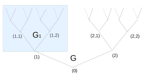
Figure 1: Example of (a portion of) an irregular Bethe Lattice $G$ of degree $q=3$ with the root vertex (0) having only 2 first neighbors. The numbers (1) and (2) in the Figure represent the vertices in the shell $n=1$, the numbers $(1,1),~{}(1,2),~{}(2,1),$ and $(2,2)$, the vertices on the second shell, and so on. Up to a change of names of the vertices, one has $G=G_{1}$, where $G_{1}$ is the (infinite) subgraph in the shaded area.

We introduce this little irregularity on our BL just to make things simpler (later on we will show how to restore the fully regular BL). From the root $({0})$ emanate 2 edges pointing at the vertices $1$ and $2$. Since $G$ is infinite, it turns out that the two equivalent infinite subgraphs $G_{1}$ and $G_{2}$ that we obtain by eliminating from $G$ the vertex $({0})$ together with its two edges, are also both equivalent to the original $G$, i.e., up to a change of name of the vertices, we have the self-similarity $G=G_{1}=G_{2}$. Note, furthermore, that $G_{1}$ and $G_{2}$ are each other disconnected. If we define the conditional partition function of the system $Z(\sigma_{0})$ with respect to the root $({0})$ as

$$Z(\sigma_{0}){\buildrel\;def\;\over{=}}\sum_{\{\sigma_{i},i\neq 0\}}e^{-\beta H\left[\{\sigma_{i}\}\right]},$$ (13)

where $H$ is defined similarly to Eq. (5), by using the self-similarity and the fact that $G_{1}$ and $G_{2}$ are disconnected, we get (again for simplicity we consider here only the case with no external field $H_{0}=0$)

$$Z(\sigma_{0})=\sum_{\sigma_{1},\sigma_{2}}e^{\beta J\sigma_{0}(\sigma_{1}+\sigma_{2})}Z(\sigma_{1})Z(\sigma_{2}).$$ (14)

One can feel unease with Eqs. (13) and (14) due to the fact that G is infinite, as well as $H$, and the $Z$’s. However we can get rid of the $Z$’s and any ill defined quantity when we consider the finite ratio $P(-)/P(+)=Z(-)/Z(+)$, where $P(\sigma_{0})$ stands for the probability that the spin at $({0})$ has value $\sigma_{0}$. If we define

$$e^{-2h}{\buildrel\;def\;\over{=}}\frac{P(-)}{P(+)},$$ (15)

from Eqs. (14) we arrive at the equation for $h$

$$e^{-2h}=\frac{e^{2\beta J-4h}+e^{-2\beta J}+2e^{-2h}}{e^{2\beta J}+e^{-2\beta J-4h}+2e^{-2h}}.$$ (16)

Eq. (16) has always the trivial solution $h=0$ corresponding to a zero magnetization. However, by expanding Eq. (16) for small $h$, it is easy to see that a non trivial solution $h\neq 0$ is present when $T<T_{\mathrm{BL}}$, where $T_{\mathrm{BL}}$ is the critical temperature given as solution of the equation

$$(q-1)\tanh(\beta J)=1,$$ (17)

which has solution as soon as $q>2$. In other words, the value $q=2$ represents the critical number of neighbors above which in the system there exists a phase transition. We can now physically understand why, unlike the BL, in the CT we cannot never have a spontaneous magnetization. From Eqs. (3) and (4) we see that, unlike the BL, on average, no matter how large the degree $q$ of the CT is, the connectivity $c$ of the CT is always strictly below the value $c=2$, therefore, in the CT, no matter how large its degree $q$ is, on average any spin is surrounded by an insufficient number of neighbors so that the system cannot have a spontaneous magnetization (at zero external field $H$)  . Similar conclusions apply to the Potts model [10]. The average magnetization of the spin $\sigma_{0}$ can be calculated from Eq. (15) and gives $\langle\sigma_{0}\rangle=\tanh(h)$, while, the average magnetization for the fully regular BL with $q=3$ is simply $\langle\sigma_{0}\rangle=\langle\sigma\rangle=\tanh(h\times 3/2)$. Notice however the necessity to consider the irregular BL: self-similarity, and then the possibility to have an equation for the effective field $h$, applies only to the irregular BL, not to the fully regular BL. The physicist familiar with the Cavity Method (see next subsection) recognizes in this step another way to see that $h$ is the strength felt by a spin due to all the other spins in the absence (“the cavity”) of the spin itself.

We end this subsection with the following critical note. In many textbooks of statistical mechanics, as well as in many papers that deal with a BL (regular or not), in the place of Eqs. (14) or (16), we find respectively

$$Z_{n+1}(\sigma_{0})=\sum_{\sigma_{1},\sigma_{2}}e^{\beta J\sigma_{0}(\sigma_{1}+\sigma_{2})}Z_{n}(\sigma_{1})Z_{n}(\sigma_{2}),$$ (18)

and

$$e^{-2h_{n+1}}=\frac{e^{2\beta J-4h_{n}}+e^{-2\beta J}+2e^{-2h_{n}}}{e^{2\beta J}+e^{-2\beta J-4h_{n}}+2e^{-2h_{n}}},$$ (19)

and it is often wrongly said that $Z_{n}$ stands for the partition function of that finite portion of the BL having only $n$ shells. From what we have seen all above, it should be clear that such an approach for the BL is conceptually quite wrong: $Z_{n}$ cannot be interpreted as the partition function of a finite subgraph of the BL, otherwise for $Z_{n}$ we would get again Eq. (9). At this level, the only correct meaning we can attribute here to $Z_{n}(\sigma)$ is that of the conditional partition function of an infinite subgraph self-similar to that associated to $Z_{n+1}(\sigma)$, as showed above, and, most importantly, $Z_{n+1}(\sigma)$ and $Z_{n}(\sigma)$ are the same thing. In this context, the index $n$ appearing in Eqs. (18) or (19) is a quite misleading symbol. More precisely, one should use instead $Z(\sigma_{n+1})$ and $Z(\sigma_{n})$ but, as a consequence, for the ratios we would get the same value regardless of the index: $h_{n}=h_{n+1}$. Rather, looking at Eqs. (14) or (16), as a mere numerical tool, it can be convenient to introduce the recurrent Eqs. (18) or (19) since its fixed points are equivalent to Eqs. (14) or (16), respectively. A more rigorous and general meaning to $h_{n}$ can be attributed by following the next measure-theoretical approach.

4.2 Kolmogorov’ s condition

A more rigorous approach to the BL comes from the Kolmogorov consistency theorem (see e.g., [12] and [13]) by which we can avoid to introduce any ill defined quantity but, most importantly, as we will see, the method attributes a rigorous and physical meaning to Eq. (19) and to its generalizations.

From the point of view of probability theory, solving the Ising model on the BL amounts to find all the marginal probabilities of an infinite probability space, i.e., a probability space characterized by an infinite number of random variables (in our case the spins with indices in $V$), a suitable sigma-algebra [12], and a measure $\mu$. The marginal probabilities can be calculated in turn from an infinite set of given finite dimensional marginal distributions $\mu_{n}=\mu_{|V_{n}}$, where $V_{n}$ is the set of vertices that are at distance not greater than $n$ from 0. Note however that, when we consider $\mu_{n}$, we are not dealing with a finite disconnected subgraph of the given BL; the spins of $V_{n}$ that are located on the shell $n$ are in fact in turn connected to the spins of $V_{n+1}$. The key point to be used is that, given the values of the spins on $V\setminus V_{n}$, the spins on $V_{n}$ are conditioned only by the neighboring spins, i.e., the spins of the $n+1$-th shell. In turn, given a spin $\sigma_{i}$, with $i\in V_{n}$, the effects of all its neighbor spins that are on $V\setminus V_{n}$, can be encoded via a single effective external field $h_{i}$ acting only on $\sigma_{i}$. Therefore, for the $\mu_{n}$, we look for solutions of the form

$$\mu_{n}(\{\sigma_{i},i\in V_{n}\})=e^{-\beta H_{n}+\sum_{i\in W_{n}}h_{i}\sigma_{i}}/Z_{n}$$ (20)

where $H_{n}$ is given by Eq. (5), $W_{n}=V_{n}\setminus V_{n-1}$ stands for the set of vertices of the shell $n$, and $Z_{n}$ is the normalization constant. Physically, Eq. (20) represents the first step of the Bethe-Peierls approach [2] (nowadays also known as Cavity-Method in physics [16], or Belief-Propagation in computer science [18]) in which the effects of all the spins other than those of the set $V_{n}$ are encoded in the fields $\{h_{i}\}$ to be determined self-consistently. From a strict probabilistic point of view, Eqs. (20) and (5) represent the definition of the Ising model itself on the BL. Now, as we have mentioned in Sec. II, the distinction between a sequence of probability spaces of increasing size and an infinite probability space is important. The sequence of probability spaces may or may not converge to anything, and even if it converges, it may happen that it does not converge to a probability space. The tool to investigate whether a sequence of increasing probability spaces converges to an infinite probability space is provided by the Kolmogorov consistency theorem [12]. It should be clear that on an infinite space like the BL, the probability that a given configuration of spins $\{\sigma_{i},i\in\mathbb{N}\}$ (a point-like event) is realized is zero: $\mu(\{\sigma_{i},i\in\mathbb{N}\})=0$. Therefore, when one considers an infinite probability space, the introduction of a proper sigma-algebra is not just a formal necessity. However, since here we do not need to work directly with the measure $\mu$ of the infinite space, for what follows, we can skip the introduction of the sigma-algebras. The Kolmogorov consistency theorem says that a sequence of probability spaces $(V_{n},\mu_{n})$ converges to the probability space on BL, $(V,\mu)$, if for any $n\geq 1$ one has

$$\sum_{\{\sigma_{i},i\in W_{n+1}\}}\mu_{n+1}(\{\sigma_{i},i\in V_{n+1}\})=\mu_{n}(\{\sigma_{i},i\in V_{n}\}).$$ (21)

Eqs. (20) and (21) give the functional equations for the fields $h_{i},i\in W_{n}$.

Due to the tree-like structure of the BL, Eq. (21) factorizes over independent branches allowing for a fundamental simplification. Let us apply Eqs. (20) and (21) to the same model analyzed in the previous subsection (a BL with $q=3$ in which the root vertex (0) has only two first neighbors) [14, 15]. For any given $i_{0}\in W_{n}$ we indicate with $i_{1}$ and $i_{2}$ the indices of the first two neighbors of $i_{0}$ that belong to $W_{n+1}$. We have ($H_{0}=0$)

$$\frac{e^{-\beta H_{n}(\{\sigma_{l},l\in V_{n}\})}}{Z_{n+1}}\prod_{i_{0}\in W_{n}}\sum_{\sigma_{i_{1}},\sigma_{i_{2}}}\left[e^{\beta J\sigma_{i_{0}}(\sigma_{i_{1}}+\sigma_{i_{2}})+h_{i_{1}}\sigma_{i_{1}}+h_{i_{2}}\sigma_{i_{2}}}\right]$$ (22)

$$= \frac{e^{-\beta H_{n}(\{\sigma_{l},l\in V_{n}\})}}{Z_{n}}\prod_{i_{0}\in W_{n}}e^{h_{i_{0}}\sigma_{i_{0}}}~{}~{}$$

From Eq. (22), for any $i_{0}\in W_{n}$ and for any values of $\sigma_{i_{0}}$, we have an equation for the field $h_{i_{0}}$ as a function of the fields $h_{i_{1}}$ and $h_{i_{2}}$

$$\frac{Z_{n}}{Z_{n+1}}\sum_{\sigma_{i_{1}},\sigma_{i_{2}}}e^{\beta J\sigma_{i_{0}}(\sigma_{i_{1}}+\sigma_{i_{2}})+h_{i_{1}}\sigma_{i_{1}}+h_{i_{2}}\sigma_{i_{2}}}=e^{h_{i_{0}}\sigma_{i_{0}}},$$

from which, by evaluating the cases $\sigma_{i_{0}}=+1$ and $\sigma_{i_{0}}=-1$ we get

$$e^{-2h_{i_{0}}}=$$ (23)

$$\frac{e^{2\beta J-h_{i_{1}}-h_{i_{2}}}+e^{-2\beta J+h_{i_{1}}+h_{i_{2}}}+e^{h_{i_{1}}-h_{i_{2}}}+e^{h_{i_{2}}-h_{i_{1}}}}{e^{2\beta J+h_{i_{1}}+h_{i_{2}}}+e^{-2\beta J-h_{i_{1}}-h_{i_{2}}}+e^{h_{i_{1}}-h_{i_{2}}}+e^{h_{i_{2}}-h_{i_{1}}}}.$$

It is immediate to verify that Eqs. (23) reduce to Eq. (19) for the choice $h_{i_{0}}=h_{i_{1}}=h_{i_{2}}=h_{n}$. Besides to be rigorous, this approach, based on the Kolmogorov consistency theorem, shows us that a possible non homogeneous solution for the effective fields $\{h_{i}\}$, periodic or not, is not an artifact of the theory: an effective field which depends on the index vertex is in correspondence with a non homogeneous marginal probability which depends on the index vertex too.

In the context of the Cavity and Belief Propagation methods, Eqs. (23) are better known in another form more suited for an intuitive interpretation of the effective fields as messages $h_{i\to j}$ passing from a vertex $i$ to a neighbor vertex $j$; see Fig. (2).

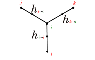
Figure 2: Graphical message-passing interpretation of the effective fields. Each field $h_{i\to l}$ is in correspondence with an edge $(i,l)=(l,i)\in E$ (recall that our BL $G$ is an undirected graph). The field/message $h_{i\to l}$, emanating from $i$, as seen from Eq. (24), is a function of all the other fields/messages arriving to $i$: $h_{j\to i}$ and $h_{k\to i}$. The correspondence between the fields appearing in Eqs. (23) and those of Eqs. (24) is: $h_{i\to l}=h_{i_{0}}$, $h_{j\to i}=h_{i_{1}}$, and $h_{k\to i}=h_{i_{2}}$. Note that, in general, we can attribute a direction to the fields/messages $h_{i\to l}$ even if the graph $G$ is an undirected graph (i.e., for any $(i,j)\in E$ we have $(i,j)=(j,i)\in E$).

By using $\tanh^{-1}(x)=1/2\log[(1+x)/(1-x)]$, valid for $|x|<1$, it is easy to see that Eqs. (23) can be rewritten as

$$h_{i\to l} = \tanh^{-1}\left[\tanh(\beta J)\tanh(h_{j\to i})\right]+\tanh^{-1}\left[\tanh(\beta J)\tanh(h_{k\to i})\right].$$ (24)

More in general, the equation for a an Ising model built on a generic BL, regular or not, having generic couplings $J_{ij}$ and an external field $H_{0}$, reads as

$$h_{i\to j}=\sum_{k\in\partial i\setminus j}\tanh^{-1}\left[\tanh(\beta J_{ij})\tanh(\beta H_{0}+h_{k\to i})\right],~{}~{}$$ (25)

where $\partial i$ stands for the set of the first neighbors of the vertex $i$.

The developments about the convergence and algorithmic issues around Eqs. (25), as well as their applications in physics, computer science, and statistical inference are huge (see e.g. [16], [17], [18]). Here we wanted just to stress the equivalence between the Cavity/Belief-Propagation approaches and a rigorous method based on the Kolmogorov consistency theorem.

5 Last observation

From the previous Section, we see that we could re-interpret the (infinite) BL, as the thermodynamic limit of (finite) CT’s having specific “boundary conditions” determined by the fields $h_{i}$ solution of Eqs. (20) and (21), as shown in [19]. However, this point of view is a quite poor physical one (a system whose thermodynamic limit exists only for a specific boundary condition) and, pedagogically, very inconvenient.

6 conclusions

We have reviewed critically the concepts and the applications of CT and BL in statistical mechanics emphasizing their very different features. We have pointed out that careful must be paid especially in the case of a BL, an infinite space, where serious misuses and misunderstandings are currently seen in both textbooks and journal papers due to a ill mathematical approach to the BL. We have then illustrated for the BL case two alternative approaches which are rigorous and free of dangerous ambiguities based respectively on self-similarity and the Kolmogorov consistency theorem, pointing out the link of the latter with the Cavity and Belief Propagation methods, more known to the physics community. We hope that this critical review paper, where concepts and tools from physics and mathematics (too often kept apart) are used, might reduce the quite widespread misuse and conceptual errors around CT and BL.

References

References

- [1] A. Cayley, Arthur, Desiderata and suggestions: No. 2. The Theory of groups: graphical representation. Amer. J. Math. (2): 174 (1878).
- [2] H. A. Bethe, Statistical theory of superlattices, Proc. Roy. Soc. London Ser A, 150, 552 (1935).
- [3] P. Erds, A. Rnyi, Publ. Math. Debrecen 6, 290 (1959).
- [4] R. Albert, A.L. Barb´asi, Rev. Mod. Phys. 74, 47 (2002); S.N. Dorogovtsev, J.F.F. Mendes, Evolution of Networks (University Press: Oxford, 2003); M. E. J. Newman, SIAM Review 45, 167 (2003); S. N. Dorogovtsev, Lectures on Complex Networks (Oxford Master Series in Statistical, Computational, and Theoretical Physics, 2010); S. N. Dorogovtsev, A. V. Goltsev, J.F.F. Mendes, Rev. Mod. Phys. 80, 1275 (2008).
- [5] R. J. Baxter, Exact Solved Models in Statistical Mechanics (Academic Press, London, 1982).
- [6] T. P. Eggarter, Phys. Rev. B 9, 2989 (1974).
- [7] H. Matsuda, Progr. Theor. Phys. 51 1053 (1973).
- [8] E. Muller-Hartmann, and J. Zittartz, Phys. Rev. Lett. 33, 893 (1974).
- [9] F. Y. Wu, J. Phys. A: Math. Gen. 9 593 (1976).
- [10] L. Turban, Phys. Lett. 78A 404 (1980).
- [11] C. Domb, Ising model Phase Transitions and Critical Phenomena Vol. 3 Ed. C. Domb. and M. S. Green (London: Academic Press) 357 (1974).
- [12] A. N. Shiryaev, Probability (New York, Springer, 1984).
- [13] Y. G. Sinai, Theory of phase transitions: rigorous results, (Oxford ; New York : Pergamon Press, 1982).
- [14] H. O. Georgii, Gibbs measures and phase transitions (Walter de Gruyter, Berlin, 1988).
- [15] P. M. Bleher, J. Ruiz and V. A. Zagrebnov, J. Stat. Phys. 79, 473 (1995).
- [16] M. Mezard, G. Parisi, Eur. Phys. J. B 20, 217-233 (2001).
- [17] R. Zecchina, O. C. Martin, and R. Monasson, Statistical mechanics methods and phase transitions in optimization problems Theoretical Computer Science, 3, 265 (2001).
- [18] J. S. Yedidia, J.S.; W. T. Freeman, Understanding Belief Propagation and Its Generalizations In Lakemeyer, Gerhard; Nebel, Bernhard. Exploring Artificial Intelligence in the New Millennium. Morgan Kaufmann, 239 (2003).
- [19] C. J. Thomposon, J. Stat. Mech. 27, 441 (1982).