Ab initio studies of electron correlation and Gaunt interaction effects in boron isoelectronic sequence using coupled-cluster theory

Abstract

In this paper, we have studied electron correlation and Gaunt interaction effects in ionization potentials (IPs) and hyperfine constants A of 2p${}^{2}P_{1/2}$ and 2p${}^{2}P_{3/2}$ states along with the fine structure splitting (FSS) between them for boron isoelectronic sequence using relativistic coupled-cluster (RCC) method. The range of atomic number Z has been taken from 8 to 21. Gaunt contributions are presented at both Dirac-Fock (DF) and coupled-cluster (CC) levels of calculations. The Gaunt corrected correlated results of the IPs and the FSS are compared with the results of NIST. Important correlation contributions like core correlation, core polarisation, pair correlation etc. are studied for hyperfine constants A. Many distinct features of correlation and relativistic effects are observed in these studies. With best of our knowledge, within Gaunt limit, most of the hyperfine constants are presented for the first time in the literature.

I Introduction

Researches in isoelectronic sequences of lighter atoms have been a subject of recent interest to study various atomic properties of low-lying atomic states and the transitions between them pachucki ; yerokhin ; hao . Accurate estimations of these properties require correlation corrections with Breit and quantum electrodynamic (QED) effects jie . However, individual studies of all these effects are necessary to realize the relative strengths between them with increasing atomic number for different isoelectronic sequences. To implement these effects in different many-body theories, suitable form of matrix elements of their operators are necessary. From our literature survey, we have found a number of such formulations for the Breit operator mann ; kim ; pyper ; hinze ; grant . However, in our work, we have implemented the Gaunt interaction which is the magnetic part of the Breit interaction grant and is considered to be an order of magnitude larger than the other part, called as the retardation part mann . Hence the Gaunt interaction is considered to provide a useful approximation to the Breit interaction mann . The matrix element of the Gaunt operator is reformulated to add with the coulomb operator in a self consistent approach at both the DF as well as the CC level of calculations.

In recent years, a number of theoretical calculations have been performed on boron isoelectronic sequence which take into account the Breit interaction in the atomic Hamiltonian hao ; jie ; li ; zhang ; rancova ; koc1 ; koc2 ; koc3 ; koc4 ; tachiev ; safronova1 ; safronova2 ; safronova3 ; merkelis ; galavis ; zheng . These calculations have been performed using different many-body approaches like configuration-interaction technique hao ; rancova ; galavis , multi-configuration Dirac-Fock method jie ; li ; zhang , weakest bound electron potential model theory zheng , relativistic multireference configuration-interaction technique koc1 ; koc2 ; koc3 ; koc4 , multiconfiguration Hartree-Fock method tachiev , relativistic many-body perturbation theory safronova1 ; safronova2 ; safronova3 ; merkelis etc. Eliav et al. have implemented Breit operator in the CC theory but treated only four members of this sequence to calculate the IPs and the FSS eliav . Recently, the RCC calculations of this sequence have been performed by Nataraj et al. nataraj for Mg VIII, Si X and S XII. They have performed the RCC calculations on different transition properties among some low-lying states of these ions in the basis of Dirac-Coulomb Hamiltonian. In their paper, they have highlighted the requirement of the Breit interaction in the fine structure splitting of 2${}^{2}P$ term of this sequence.

Isoelectronic sequences are also very useful to study the trends of relativistic and the different correlation effects in the hyperfine properties of different ions panigrahy . Panigrahy et al. have investigated different correlation mechanisms on the magnetic dipole hyperfine constants (A) of Li like systems by many-body perturbation theory panigrahy . As members of boron isoelectronic sequence, hyperfine constants of C II, N III and O IV have been calculated by Jönsson et al. jonsson . The QED and the interelectronic interaction corrections in hyperfine properties have been analyzed by Oreshkina et al. by large-scale configuration-interaction Dirac-Fock-Sturm method for few members of this sequence glazov .

The purpose of this present paper is to analyze the correlation and the Gaunt effects in the calculations of the IPs, the hyperfine constants A of 2p${}^{2}P_{1/2}$ and 2p${}^{2}P_{3/2}$ states and the FSS between them for boron like systems using relativistic coupled-cluster approach. The systematic investigations of both these effects with increasing atomic number can provide a comparative information about their contributions in the calculations of these properties. Comparisons of the Gaunt contributions at both the DF and the CC levels of calculations have been explicitly studied to test the correlation effects on these. Our final calculated results of the IPs and the FSS including correlation and Gaunt effects, are compared with the results of National Institute of Standards and Technology (NIST) nist . Graphical variations of these effects are shown with increasing atomic number. The RCC method, applied in these calculations, consist of single, double and partial triple excitations dixit . Different types of correlation effects like core correlation, pair correlation and core polarisation in the hyperfine constants are tabulated and are plotted to observe their variations w.r.t. Z.

II Theory

II.1 Matrix element of Gaunt interaction operator

The Breit interaction, introduced by Breit breit , is the first relativistic correction of the Coulomb interaction. The frequency independent form of the Breit interaction between two electrons, indicated by ’1’ and ’2’, is given by

$$H_{B}=-\frac{\overrightarrow{\alpha_{1}}\cdot\overrightarrow{\alpha_{2}}}{r_{12}}+\frac{1}{2}\left[\frac{\overrightarrow{\alpha_{1}}\cdot\overrightarrow{\alpha_{2}}}{r_{12}}-\frac{(\overrightarrow{\alpha_{1}}\cdot\overrightarrow{r_{12}})(\overrightarrow{\alpha_{2}}\cdot\overrightarrow{r_{12}})}{r^{3}_{12}}\right]$$ (1)

where $\alpha_{1}$ and $\alpha_{2}$ are the corresponding Dirac matrices and $r_{12}$ is the distance of separation between the two electrons reither . The overall Breit interaction is contributed by magnetic part, called Gaunt interaction gaunt as stated earlier, represented by the first term of Eq. 2.1 and the other part which includes the retardation effect, called as retardation part, represented by the remaining part of this equation.

Including Gaunt interaction with Coulomb interaction, the atomic Hamiltonian of a N electron system is written in the form

$$H=\sum_{i=1}^{N}\left(c\overrightarrow{\alpha_{i}}\cdot\overrightarrow{p_{i}}+\left(\beta_{i}-1\right)c^{2}+V_{nuc}(r_{i})+\sum_{j<i}^{N}\left(\frac{1}{r_{ij}}-\frac{\overrightarrow{\alpha_{i}}\cdot\overrightarrow{\alpha_{j}}}{r_{ij}}\right)\right).$$ (2)

The irreducible tensor operator form of the Gaunt interaction is given by pyper ; grant

$$B_{g}=\sum_{\nu,L}(-1)^{\nu+L}V_{\nu}(1,2)\left[\textbf{X}^{((1\nu)L)}(1).\textbf{X}^{((1\nu)L)}(2)\right]$$ (3)

where $\nu=L-1$, $L$ or $L+1$ and $\textbf{X}^{((1\nu)L)}(1)=\left[\bm{\alpha}_{1}\textbf{C}^{(\nu)}(1)\right]^{(L)}$ pyper . In the long wavelength approximation pyper ,

$$V_{\nu}(1,2)=\frac{r^{\nu}_{<}}{r^{\nu+1}_{>}}$$ (4)

where $r_{<}/r_{>}=min/max(r_{1},r_{2})$.

The knowledge of general two electron matrix element of the Gaunt operator is necessary to include this effect in the CC theory which is derived from Ref. pyper and is given as follows:

$$\langle A_{1}B_{2}|B_{g}|C_{1}D_{2}\rangle = \langle A_{1}B_{2}|\sum_{\nu,L}(-1)^{\nu+L}V_{\nu}(1,2)\left[\textbf{X}^{((1\nu)L)}(1).\textbf{X}^{((1\nu)L)}(2)\right]|C_{1}D_{2}\rangle$$ (9)

$$= \sum_{L,M}(-1)^{j_{A}-m_{A}+j_{B}-m_{B}+L-M}\left(\begin{array}[]{ccc}j_{A}&L&j_{C}\\ -m_{A}&M&m_{C}\\ \end{array}\right)\left(\begin{array}[]{ccc}j_{B}&L&j_{D}\\ -m_{B}&-M&m_{D}\\ \end{array}\right)$$

$$\times X^{L}(ABCD).$$ (10)

Here operator strength, $X^{L}(ABCD)$ is written in the following form:

$$X^{L}(ABCD) = (-1)^{j_{A}+j_{B}+L+1}\sqrt{(2j_{A}+1)(2j_{B}+1)(2j_{C}+1)(2j_{D}+1)}\left(\begin{array}[]{ccc}j_{A}&L&j_{C}\\ \frac{1}{2}&0&-\frac{1}{2}\\ \end{array}\right)\left(\begin{array}[]{ccc}j_{B}&L&j_{D}\\ \frac{1}{2}&0&-\frac{1}{2}\\ \end{array}\right)$$ (15)

$$\times \left[\sum^{L+1}_{\nu=L-1}\Pi^{o}(\kappa_{A},\kappa_{C},\nu)\Pi^{o}(\kappa_{B},\kappa_{D},\nu)\sum^{4}_{\mu=1}r^{\nu}_{\mu}(ABCD)R^{\nu}_{\mu}(ABCD)\right].$$ (16)

The factor

$$\Pi^{o}(\kappa_{A},\kappa_{C},\nu)=\frac{1}{2}\left[1+a_{A}a_{C}(-1)^{j_{A}+j_{C}+\nu}\right]$$ (17)

is associated with the parity selection rule of Gaunt interaction operator which is opposite to the coulomb parity selection rule. The values of $a_{A}$ and $a_{C}$ are +1 or $-$1 according to the positive or negative kappa values, respectively. The coefficients $r^{\nu}_{\mu}(ABCD)$ and the radial integrals $R^{\nu}_{\mu}(ABCD)$ are presented in Table I and Table II, respectively for values of $\mu$=1, 2, 3 or 4. For Table I, we have

$$P=\begin{cases}\dfrac{1}{L(2L-1)}\hskip 88.2037ptfor\hskip 14.22636pt\nu=L-1\\ -\dfrac{(\kappa_{A}+\kappa_{C})(\kappa_{B}+\kappa_{D})}{L(L+1)}\hskip 28.45274ptfor\hskip 14.22636pt\nu=L\\ \dfrac{1}{(L+1)(2L+3)}\hskip 59.75095ptfor\hskip 14.22636pt\nu=L+1,\end{cases}$$ (18)

$\overline{k}=\kappa_{C}-\kappa_{A}$ and $\overline{k^{\prime}}=\kappa_{D}-\kappa_{B}$. $\dfrac{P_{A}(r)}{r}$ and $\dfrac{Q_{A}(r)}{r}$ are the large and small components of the radial part of the wavefunctions, respectively pyper .

At the Dirac-Fock level, we need the knowledge of direct and exchange matrix elements of this operator which are obtained by replacing $A=A$, $B=B$, $C=A$ and $D=B$; and $A=A$, $B=B$, $C=B$ and $D=A$, respectively grant . However, the direct contribution to the Gaunt interaction is zero mann . So using the algebras of 3-$j$ symbols from Ref. grant , we give the exchange matrix element of this operator as follows:

$$\langle A_{1}B_{2}|B_{g}|B_{1}A_{2}\rangle=\sum_{L}(2j_{B}+1)\left(\begin{array}[]{ccc}j_{A}&L&j_{B}\\ \frac{1}{2}&0&-\frac{1}{2}\\ \end{array}\right)^{2}\times\left[\sum^{L+1}_{\nu=L-1}\Pi^{o}(\kappa_{A},\kappa_{B},\nu)\sum^{4}_{\mu=1}r^{\nu}_{\mu}(ABBA)R^{\nu}_{\mu}(ABBA)\right].$$ (19)

The coefficients $r^{\nu}_{\mu}(ABBA)$ are presented in Table III and the radial integrals $R^{\nu}_{\mu}(ABBA)$ are obtained from Table II by replacing $A=A$, $B=B$, $C=B$ and $D=A$. For Table III, we have

$$P=\begin{cases}\dfrac{1}{L(2L-1)}\hskip 71.13188ptfor\hskip 14.22636pt\nu=L-1\\ -\dfrac{(\kappa_{A}+\kappa_{B})^{2}}{L(L+1)}\hskip 56.9055ptfor\hskip 14.22636pt\nu=L\\ \dfrac{1}{(L+1)(2L+3)}\hskip 42.67912ptfor\hskip 14.22636pt\nu=L+1\end{cases}$$

and $\overline{k}=-\overline{k^{\prime}}=\kappa_{B}-\kappa_{A}$.

Table 1: Coefficients $r^{\nu}_{\mu}(ABCD)$

	$\nu=L-1$	$\nu=L$	$\nu=L+1$
$\mu=1$	$P(L+\overline{k})(L+\overline{k^{\prime}})$	$P$	$P(\overline{k}-L-1)(\overline{k^{\prime}}-L-1)$
$\mu=2$	$P(L-\overline{k})(L-\overline{k^{\prime}})$	$P$	$P(\overline{k}+L+1)(\overline{k^{\prime}}+L+1)$
$\mu=3$	$P(L+\overline{k})(\overline{k^{\prime}}-L)$	$P$	$P(\overline{k}-L-1)(\overline{k^{\prime}}+L+1)$
$\mu=4$	$P(\overline{k}-L)(L+\overline{k^{\prime}})$	$P$	$P(\overline{k}+L+1)(\overline{k^{\prime}}-L-1)$

Table 2: Radial integrals $R^{\nu}_{\mu}(ABCD)$

	$\nu=L-1$, $L$ or $L+1$
$\mu=1$	$\int^{\infty}_{0}\int^{\infty}_{0}P_{A}(r_{1})Q_{C}(r_{1})V_{\nu}(1,2)P_{B}(r_{2})Q_{D}(r_{2})dr_{1}dr_{2}$
$\mu=2$	$\int^{\infty}_{0}\int^{\infty}_{0}Q_{A}(r_{1})P_{C}(r_{1})V_{\nu}(1,2)Q_{B}(r_{2})P_{D}(r_{2})dr_{1}dr_{2}$
$\mu=3$	$\int^{\infty}_{0}\int^{\infty}_{0}P_{A}(r_{1})Q_{C}(r_{1})V_{\nu}(1,2)Q_{B}(r_{2})P_{D}(r_{2})dr_{1}dr_{2}$
$\mu=4$	$\int^{\infty}_{0}\int^{\infty}_{0}Q_{A}(r_{1})P_{C}(r_{1})V_{\nu}(1,2)P_{B}(r_{2})Q_{D}(r_{2})dr_{1}dr_{2}$

Table 3: Coefficients $r^{\nu}_{\mu}(ABBA)$

	$\nu=L-1$	$\nu=L$	$\nu=L+1$
$\mu=1$	$-P(\overline{k}^{2}-L^{2})$	$P$	$-P(\overline{k}^{2}-(L+1)^{2})$
$\mu=2$	$-P(\overline{k}^{2}-L^{2})$	$P$	$-P(\overline{k}^{2}-(L+1)^{2})$
$\mu=3$	$-P(\overline{k}+L)^{2}$	$P$	$-P(\overline{k}-(L+1))^{2}$
$\mu=4$	$-P(\overline{k}-L)^{2}$	$P$	$-P(\overline{k}+(L+1))^{2}$

II.2 Coupled-Cluster theory

The CC method is one of the most powerful highly correlated many-body method due to its all order structure to account the correlation effects lindgren ; dutta . This method is used here for the one valence electron and has been described in details elsewhere lindgren ; mukherjee ; Haque ; Pal ; ccsdt ; sahoo1 ; dixit .

According to the CC theory, the correlated wavefunction of a single valance atomic state having valance orbital ’$v$’ is written in the form

$$|\Psi_{v}\rangle=e^{T}\{1+S_{v}\}|\Phi_{v}\rangle$$ (20)

Here, $|\Phi_{v}\rangle$ is the corresponding DF state. $T$ is the closed shell cluster operator which considers excitations from the core orbitals and $S_{v}$ is the open shell cluster operator corresponding to the valence electron ’$v$’ sahoo1 .

The correlated expectation value of an operator $\hat{O}$ at any particular atomic state $\Psi_{v}$ can be written as

$$O^{CC}_{vv} = \frac{\langle\Psi_{v}|\hat{O}|\Psi_{v}\rangle}{\langle\Psi_{v}|\Psi_{v}\rangle}$$ (21)

$$= \frac{\langle\Phi_{v}|\{1+S^{{\dagger}}_{v}\}\overline{O}\{1+S_{v}\}|\Phi_{v}\rangle}{\langle\Phi_{v}|\{1+S^{{\dagger}}_{v}\}e^{T^{{\dagger}}}e^{T}\{1+S_{v}\}|\Phi_{v}\rangle}$$

where $\overline{O}=e^{T^{{\dagger}}}Oe^{T}$.

II.3 Hyperfine constant A

The hyperfine constant A of a state represented by $|JM\rangle$ is given by the following expression:

$$A=\mu_{N}g_{I}\frac{\langle J||{\textbf{T}^{(1)}}||J\rangle}{\sqrt{J(J+1)(J+2)}}$$ (22)

where $\mu_{N}$ is the nuclear magneton and $g_{I}$ is the g-factor of the nucleus having nuclear spin I sahoo1 ; gopal . The operator $\textbf{T}^{(1)}$ and the single-particle reduced matrix element of the electronic part of this operator is defined in Ref. sahoo2 ; rajat .

III Results and Discussions

The CC calculations are based on the generation of DF orbitals. Therefore, accurate descriptions of the radial part of the orbital wavefunctions at the DF level is one of the building blocks for accurate calculations. Here, these orbitals are considered to be gaussian type orbitals (GTOs) and are generated in the environment of $V^{N-1}$ potential of Dirac-Coulomb Hamiltonian where N is the number of electrons of each single valance system sahoo1 . The radial wavefunctions are generated on 750 grid points which follow, $r_{i}=r_{0}\left[e^{h(i-1)}-1\right]$ with $r_{0}=2\times 10^{-6}$ and h=0.05. The nuclei are considered to obey Fermi type distribution function sahoo1 . The GTOs are obtained by using universal basis parameters: $\alpha_{0}$ and $\beta$ sahoo1 ; gopal . These parameters, presented in Table IV, are optimized for each system with respect to the wavefunctions obtained from GRASP 2 code where DF equations are solved using numerical technique parpia .

In the DF calculations, the number of bases are taken as 30, 25, and 20 for s, p and d symmetries, respectively. However, in the CC calculations, 12, 11 and 10 number of the bases are used including all the bound orbitals for s, p and d symmetries, respectively. These number of symmetries and bases are chosen in accordance with the numerical convergence of the core correlation energies. In our discussions, the DF results are calculated for Dirac-Coulomb Hamiltonian. Also, correlation contributions ($\Delta^{corr}$) are calculated by the differences between the CC and the DF results for the Dirac-Coulomb Hamiltonian, i.e., Coulomb correlations. But the Gaunt contributions ($\Delta^{Gaunt}$) are calculated by the differences between the CC results for the Dirac-Coulomb-Gaunt Hamiltonian and the Dirac-Coulomb Hamiltonian. The percentage correlation contributions ($\%$ $\Delta^{corr}$) and Gaunt contributions ($\%$ $\Delta^{Gaunt}$) are evaluated with respect to the DF results and the CC results, respectively, for the Dirac-Coulomb Hamiltonian.

In Table V, our calculated IPs at the DF level are presented along with $\Delta^{corr}$ and $\Delta^{Gaunt}$. The final results which are the sum of these three, i.e., DF+$\Delta^{corr}$+$\Delta^{Gaunt}$, are compared with the results of NIST in the same table nist . Except Ca XVI, the final calculated IPs are in good agreement with the NIST results. However, our results for the former element are within the uncertainty limits (about $\pm$16000 cm^-1) of the experimental measurements jie . From Table V, one can see $\Delta^{Gaunt}$ are negative everywhere and with increasing atomic number their absolute values increase monotonically whereas positive values of $\Delta^{corr}$ decrease and become negative at $Z\geq 17$ and $Z\geq 18$ for 2p${}^{2}P_{1/2}$ and 2p${}^{2}P_{3/2}$ states, respectively. According to Eliav et al, for Z=10, the estimated correlation contributions for 2p${}^{2}P_{1/2}$ and 2p${}^{2}P_{3/2}$ states are 4806.93 and 4865.75 cm^-1, respectively whereas for Z=18 these values are $-$1104.40 and $-$59.26 cm^-1, respectively which are in well agreement with our calculations. The IP of 2p${}^{2}P_{3/2}$ state for Z=16 calculated at the DF level is close to the total result. For this case, the absolute values of $\Delta^{Gaunt}$ and $\Delta^{corr}$ are relatively close to each other, but their signs are opposite. So the overall contribution of these two effects do not change the DF result significantly. However, the wavefunctions responsible for the DF and final results are entirely different which is observed in the calculations of the hyperfine properties as discussed later in the present paper. As seen from the table, at higher Z values of the sequence, $\Delta^{Gaunt}$ are comparable with $\Delta^{corr}$ in the determinations of the IPs.

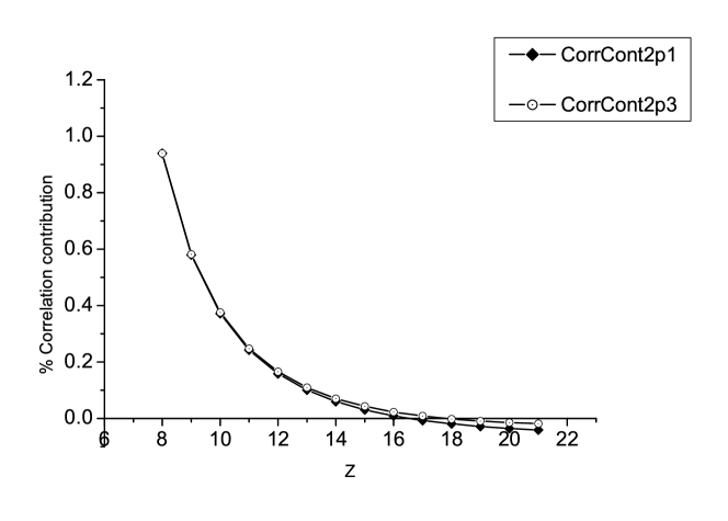
Figure 1: Percentage correlation contributions (CorrCont) to the IPs of 2p${}^{2}P_{1/2}$ (2p1) and 2p${}^{2}P_{3/2}$ (2p3) states.

In Fig. 1 and Fig. 2, graphical variations of $\%$ $\Delta^{corr}$ and $\%$ $\Delta^{Gaunt}$ to the IPs w.r.t. Z are presented, respectively. The $\%$ $\Delta^{corr}$ first decrease rapidly and then vary slowly whereas absolute values of the $\%$ $\Delta^{Gaunt}$ increase linearly with increasing Z. In Fig. 1, the $\%$ $\Delta^{corr}$ curve of 2p${}^{2}P_{1/2}$ states shows slightly more fall compare to the curve of 2p${}^{2}P_{3/2}$ states. Even from Fig. 2, one can see the curve of 2p${}^{2}P_{1/2}$ is slightly more steep than that of 2p${}^{2}P_{3/2}$. So from these two figures, it is obvious that with increasing Z, both $\%$ $\Delta^{Gaunt}$ and $\%$ $\Delta^{corr}$ are more effective for the former states than that of the latter states in determining the IPs. The correlation and the Gaunt effects are found to vary from +1$\%$ to $-$0.1$\%$ and $-$0.01$\%$ to $-$0.04$\%$, respectively in the IPs.

In Table VI, the FSS between 2p${}^{2}P_{1/2}$ and 2p${}^{2}P_{3/2}$ states are tabulated with correlation and Gaunt contributions. The final results are compared with the results of NIST nist . From this table one can find, except at Z=8, $\Delta^{corr}$ are negative for rest of the Z and their absolute values increase with increasing Z. But $\Delta^{Gaunt}$ are negative for all the Z and their absolute values also increase with increasing Z. In the cases of Mg VIII, Si X and S XII, our CC results (DF+$\Delta^{corr}$) are in good agreement with the results of Nataraj et al. nataraj . However, the significant improvement of the final results due to the inclusion of the Gaunt interaction not only for these but also for the other ions are noted from this table.

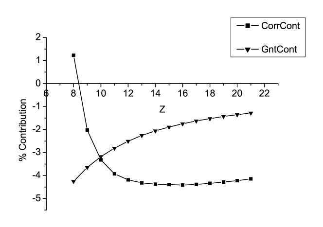
Figure 3: Percentage correlation (CorrCont) and Gaunt contributions (GntCont) to the FSS between 2p${}^{2}P_{1/2}$ and 2p${}^{2}P_{3/2}$ states.

In Fig. 3, variation of percentage correlation and Gaunt contributions to the FSS are plotted w.r.t. Z. This figure highlights that from Z=9, absolute values of $\%$ $\Delta^{corr}$ first increase rapidly, then slow down and after Z=16, decrease slowly whereas absolute values of $\%$ $\Delta^{Gaunt}$ decrease systematically with increasing Z. Up to Z=9, $\%$ $\Delta^{Gaunt}$ dominate over $\%$ $\Delta^{corr}$, but after that the case is reverse. From this figure. one can see, $\%$ $\Delta^{corr}$ vary from +1.5$\%$ to $-$4.5$\%$ and $\%$ $\Delta^{Gaunt}$ vary from $-$4.5$\%$ to $-$1.5$\%$ in the FSS. These show that both $\Delta^{corr}$ and $\Delta^{Gaunt}$ are very much important in accurate determinations of the FSS compare to the IPs.

In Table VII, the hyperfine constants A are tabulated with correlation and Gaunt effects. In these calculations, the most stable isotopes of the each elements are chosen and the $g_{I}$ values of these isotopes are calculated from Ref. raghavan . Here, we consider the magnitudes of the $g_{I}$ values neglecting their signs and are presented in the same table. The multiconfiguration Dirac-Hartree-Fock results within Breit-Pauli approximation by Jönsson et al. for O IV (Z=8) of 2p${}^{2}P_{1/2}$ and 2p${}^{2}P_{3/2}$ states are 1647 and 324 MHz, respectively which are in good agreement with our final results jonsson . This table clearly shows correlation contributions arise as a dominating mechanism compared to the Gaunt contributions in the determinations of the hyperfine constants. Contrary to the IP, the DF result differ significantly from the final result of 2p${}^{2}P_{3/2}$ state for Z=16 due to the difference of the wavefunctions between two different level of calculations.

In Table VIII, important correlation contributions from core correlation ($\overline{O}-O$), pair correlation ($\overline{O}S_{1v}$+c.c.) and the lowest order core polarisation ($\overline{O}S_{2v}$+c.c.) along with correlations from the terms $S^{{\dagger}}_{2v}\overline{O}S_{2v}$ +c.c. and normalization corrections to the hyperfine constants are reported gopal . Here c.c. stands for complex conjugate of the corresponding term gopal . The remaining correlation contributions come from the terms like $S^{{\dagger}}_{1v}\overline{O}S_{1v}$ +c.c. and $S^{{\dagger}}_{1v}\overline{O}S_{2v}$ +c.c. and the other effective two-body terms gopal which are not discussed here due to their relatively small contributions. As seen from this table, the pair correlation effects are positive, but core correlation and core polarisation effects are opposite in sign between the fine structure states. For lighter ions, considerable correlation contributions are found to occur from the terms $S^{{\dagger}}_{2v}\overline{O}S_{2v}$ +c.c. for 2p${}^{2}P_{3/2}$ states.

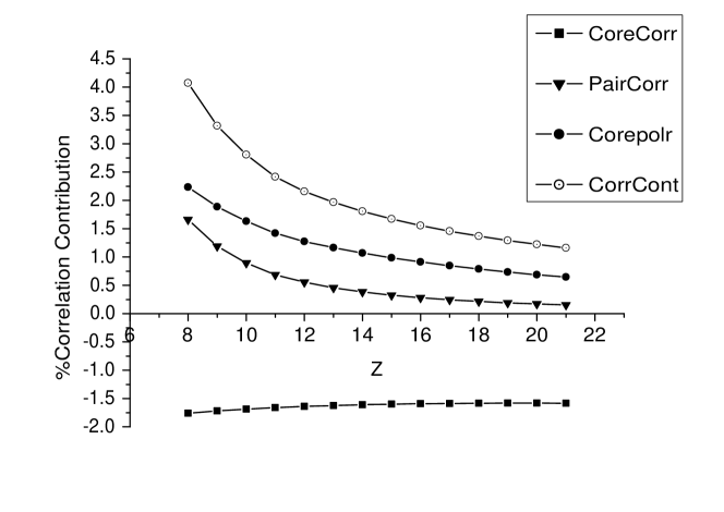
Figure 4: Percentage of total correlation contributions (TotCorrCont) with core correlation (CoreCorr), pair correlation (PairCorr) and core polarisation (CorePolr) effects in the hyperfine constants A of 2p${}^{2}P_{1/2}$ states.

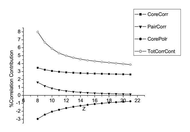
Figure 5: Percentage of total correlation contributions (TotCorrCont) with core correlation (CoreCorr), pair correlation (PairCorr) and core polarisation (CorePolr) effects in the hyperfine constants A of 2p${}^{2}P_{3/2}$ states.

The variation of $\%$ $\Delta^{corr}$, i.e., the percentage of total correlation contributions, w.r.t. Z to the hyperfine constants are shown in Fig. 4 and Fig. 5 along with the different correlation effects for 2p${}^{2}P_{1/2}$ and 2p${}^{2}P_{3/2}$ states, respectively. The percentage correlation contributions of the different correlation terms are calculated w.r.t. the DF results. Like the IPs, here also $\%$ $\Delta^{corr}$ first decrease rapidly and then decrease slowly with increasing Z. But unlike to the IPs, $\%$ $\Delta^{corr}$ are positive everywhere. The $\%$ $\Delta^{corr}$ of 2p${}^{2}P_{1/2}$ and 2p${}^{2}P_{3/2}$ states vary from +4.25$\%$ to +1.25$\%$ and +8$\%$ to +4$\%$, respectively. As Z increase, absolute values of the percentage correlation contributions from the different correlation terms decrease. Among these, the core correlation effects are most stable with respect to the other two correlation effects. At higher Z values, major correlations come from the core correlations and the next higher contributions come from the core polarisations.

In Table IX, Table X and Table XI, Gaunt contributions to the IPs, the FSS and the hyperfine A constants are presented, respectively at both the DF and the CC levels of calculations to show their changes due to correlation effects. From Table IX, it is seen for 2p${}^{2}P_{1/2}$ states where correlation effects on Gaunt contributions are increasing systematically, for 2p${}^{2}P_{3/2}$ states, it is increasing up to Z=15 and then start decreasing with increasing Z. The same table also shows that correlation effects on Gaunt contributions are relatively more stronger for 2p${}^{2}P_{1/2}$ states compare to the 2p${}^{2}P_{3/2}$ states. In the IP’s, correlation effects change the Gaunt contributions from the DF to the CC levels by +7.50$\%$ to +2.94$\%$ and +3.73$\%$ to $-$0.09$\%$ for 2p${}^{2}P_{1/2}$ and 2p${}^{2}P_{3/2}$ states, respectively. However, in the FSS the changes are more stronger which are about +17.34$\%$ to +15.13$\%$. As expected due to relatively large correlation effects, the dramatic changes occur in the hyperfine constants as seen from Table XI which almost exhaust the Gaunt contributions at the DF levels and provide very small to the CC levels. These changes are about +102.97$\%$ to +88.60$\%$ and +88.89$\%$ to +75.61$\%$ for 2p${}^{2}P_{1/2}$ and 2p${}^{2}P_{3/2}$ states, respectively.

Table 4: Universal basis parameters $\alpha_{0}$ and $\beta$

Z	8	9	10	11	12	13	14	15	16	17	18	19	20	21
$\alpha_{0}$	0.00225	0.00275	0.00325	0.00350	0.00425	0.00525	0.00625	0.00725	0.00825	0.00925	0.01025	0.01125	0.01225	0.01325
$\beta$	2.73	2.73	2.73	2.73	2.73	2.73	2.73	2.73	2.73	2.73	2.73	2.73	2.73	2.73

Table 5: Calculated IPs with correlation and Gaunt effects along with the comparisons with the NIST results (in cm^-1).

Z	State	DF	$\Delta^{corr}$	$\Delta^{Gaunt}$	Totala	NISTb
8	2p${}^{2}P_{1/2}$	618204.38	5808.89	-73.72	623939.55	624382
	2p${}^{2}P_{3/2}$	617770.18	5803.55	-55.03	623518.70	623996
9	2p${}^{2}P_{1/2}$	915988.05	5307.30	-128.55	921166.80	921430
	2p${}^{2}P_{3/2}$	915158.69	5324.07	-98.90	920383.86	920686
10	2p${}^{2}P_{1/2}$	1269209.36	4716.60	-204.62	1273721.34	1273820
	2p${}^{2}P_{3/2}$	1267767.50	4764.47	-160.38	1272371.59	1272513
11	2p${}^{2}P_{1/2}$	1677809.33	4060.48	-305.45	1681564.36	1681700
	2p${}^{2}P_{3/2}$	1675470.31	4152.24	-242.35	1679380.20	1679565
12	2p${}^{2}P_{1/2}$	2141817.07	3385.86	-433.87	2144769.06	2145100
	2p${}^{2}P_{3/2}$	2138220.31	3536.45	-347.56	2141409.20	2141798
13	2p${}^{2}P_{1/2}$	2661309.44	2677.04	-593.23	2663393.25	2662650
	2p${}^{2}P_{3/2}$	2656009.14	2905.80	-478.73	2658436.21	2657760
14	2p${}^{2}P_{1/2}$	3236356.19	1944.52	-787.29	3237513.42	3237300
	2p${}^{2}P_{3/2}$	3228811.95	2274.68	-638.94	3230447.69	3230309
15	2p${}^{2}P_{1/2}$	3867061.50	1193.76	-1019.32	3867235.94	3867100
	2p${}^{2}P_{3/2}$	3856629.52	1651.45	-830.90	3857450.07	3857401
16	2p${}^{2}P_{1/2}$	4553546.98	411.06	-1292.67	4552665.37	4552500
	2p${}^{2}P_{3/2}$	4539468.86	1032.31	-1057.46	4539443.71	4539365
17	2p${}^{2}P_{1/2}$	5295946.59	-371.31	-1610.97	5293964.31	5293800
	2p${}^{2}P_{3/2}$	5277342.47	444.22	-1321.51	5276465.18	5276390
18	2p${}^{2}P_{1/2}$	6094410.81	-1166.35	-1977.55	6091266.91	6090500
	2p${}^{2}P_{3/2}$	6070267.99	-118.69	-1625.80	6068523.50	6067844
19	2p${}^{2}P_{1/2}$	6949103.86	-1973.12	-2395.89	6944734.85	6943800
	2p${}^{2}P_{3/2}$	6918267.32	-652.16	-1973.18	6915641.98	6914783
20	2p${}^{2}P_{1/2}$	7860203.67	-2790.74	-2869.39	7854543.54	7860000
	2p${}^{2}P_{3/2}$	7821366.32	-1152.48	-2366.49	7817847.35	7823480
21	2p${}^{2}P_{1/2}$	8827901.77	-3618.45	-3401.58	8820881.74	8820000
	2p${}^{2}P_{3/2}$	8779594.34	-1616.56	-2808.45	8775169.33	8774363

^aTotal= DF+$\Delta^{corr}$+$\Delta^{Gaunt}$.

^bNIST $\rightarrow$ NIST results nist .

Table 6: Calculated FSS between 2p${}^{2}P_{1/2}$ and 2p${}^{2}P_{3/2}$ states with correlation and Gaunt effects along with the comparisons with the NIST results (in cm^-1) .

Z	DF	$\Delta^{corr}$	$\Delta^{Gaunt}$	Totala	NISTb
8	434.20	5.34	-18.69	420.85	386
9	829.36	-16.77	-29.65	782.94	744
10	1441.86	-47.87	-44.24	1349.75	1307
11	2339.02	-91.76	-63.10	2184.16	2135
12	3596.76	-150.59	-86.31	3359.86	3302
13	5300.30	-228.76	-114.50	4957.04	4890
14	7544.24	-330.16	-148.33	7065.75	6991
15	10431.98	-457.69	-188.42	9785.87	9699
16	14078.12	-621.25	-235.21	13221.66	13135
17	18604.12	-815.53	-289.46	17499.13	17410
18	24142.82	-1047.66	-351.75	22743.41	22656
19	30836.54	-1320.96	-422.71	29092.87	29017
20	38837.35	-1638.26	-502.90	36696.19	36520
21	48307.43	-2001.89	-593.13	45712.41	45637

^aTotal= DF+$\Delta^{corr}$+$\Delta^{Gaunt}$.

^bNIST $\rightarrow$ NIST results nist .

Table 7: Calculated hyperfine constants A with Correlation and Gaunt effects (in MHz).

Z	$g_{I}$	State	DF	$\Delta^{corr}$	$\Delta^{Gaunt}$	Totala
8	0.7575	2p${}^{2}P_{1/2}$	1595.69	64.98	0.03	1660.70
		2p${}^{2}P_{3/2}$	317.67	25.37	-0.02	343.02
9	5.2577	2p${}^{2}P_{1/2}$	18100.83	600.68	-0.10	18701.41
		2p${}^{2}P_{3/2}$	3598.48	239.80	-0.29	3837.99
10	0.4412	2p${}^{2}P_{1/2}$	2310.26	64.83	-0.05	2375.04
		2p${}^{2}P_{3/2}$	458.56	26.97	-0.04	485.49
11	1.4784	2p${}^{2}P_{1/2}$	11170.12	270.02	-0.49	11439.65
		2p${}^{2}P_{3/2}$	2213.27	117.65	-0.26	2330.66
12	0.3422	2p${}^{2}P_{1/2}$	3582.42	77.29	-0.20	3659.51
		2p${}^{2}P_{3/2}$	708.45	35.37	-0.10	743.72
13	1.4566	2p${}^{2}P_{1/2}$	20459.89	402.39	-1.42	20860.86
		2p${}^{2}P_{3/2}$	4037.56	191.52	-0.65	4228.43
14	1.1106	2p${}^{2}P_{1/2}$	20390.77	368.23	-1.68	20757.32
		2p${}^{2}P_{3/2}$	4014.68	183.07	-0.75	4197.00
15	2.2632	2p${}^{2}P_{1/2}$	53148.34	887.65	-5.15	54030.84
		2p${}^{2}P_{3/2}$	10438.26	461.21	-2.23	10897.24
16	0.4292	2p${}^{2}P_{1/2}$	12658.08	196.88	-1.41	12853.55
		2p${}^{2}P_{3/2}$	2479.40	106.89	-0.60	2585.69
17	0.5479	2p${}^{2}P_{1/2}$	19978.04	290.71	-2.54	20266.21
		2p${}^{2}P_{3/2}$	3902.05	164.37	-1.05	4065.37
18	0.3714	2p${}^{2}P_{1/2}$	16518.00	225.90	-2.37	16741.53
		2p${}^{2}P_{3/2}$	3216.44	132.62	-0.96	3348.10
19	0.1433	2p${}^{2}P_{1/2}$	7682.31	99.13	-1.23	7780.21
		2p${}^{2}P_{3/2}$	1491.10	60.23	-0.49	1550.84
20	0.3765	2p${}^{2}P_{1/2}$	24077.93	294.13	-4.29	24367.77
		2p${}^{2}P_{3/2}$	4657.46	184.30	-1.68	4840.08
21	1.3590	2p${}^{2}P_{1/2}$	102723.90	1191.39	-20.18	103895.11
		2p${}^{2}P_{3/2}$	19798.50	767.11	-7.75	20557.86

^aTotal= DF+$\Delta^{corr}$+$\Delta^{Gaunt}$.

Table 8: Important correlation contributions to the hyperfine constants A (in MHz).

Z	State	Core-Corra	Pair-Corrb	Core-Polrc	$S^{{\dagger}}_{2v}\overline{O}S_{2v}$	Normd
8	2p${}^{2}P_{1/2}$	-28.07	26.51	35.66	13.62	21.51
	2p${}^{2}P_{3/2}$	11.04	5.25	-9.43	15.32	4.38
9	2p${}^{2}P_{1/2}$	-311.09	215.09	341.76	119.27	270.91
	2p${}^{2}P_{3/2}$	116.17	42.50	-87.33	123.50	54.41
10	2p${}^{2}P_{1/2}$	-38.98	20.66	37.65	12.10	36.84
	2p${}^{2}P_{3/2}$	14.11	4.07	-9.41	11.76	7.32
11	2p${}^{2}P_{1/2}$	-185.61	76.62	158.66	47.50	185.94
	2p${}^{2}P_{3/2}$	65.82	15.07	-40.17	43.75	36.46
12	2p${}^{2}P_{1/2}$	-58.75	19.82	45.66	12.67	61.28
	2p${}^{2}P_{3/2}$	20.54	3.89	-11.31	11.24	11.84
13	2p${}^{2}P_{1/2}$	-331.92	93.45	238.57	61.09	357.17
	2p${}^{2}P_{3/2}$	114.83	18.28	-58.14	52.56	67.84
14	2p${}^{2}P_{1/2}$	-327.95	78.19	218.16	52.14	361.01
	2p${}^{2}P_{3/2}$	112.47	15.24	-52.42	43.65	67.27
15	2p${}^{2}P_{1/2}$	-849.01	173.54	523.73	117.76	951.09
	2p${}^{2}P_{3/2}$	288.87	33.71	-124.24	96.30	173.43
16	2p${}^{2}P_{1/2}$	-201.59	35.62	115.32	24.56	229.00
	2p${}^{2}P_{3/2}$	68.05	6.89	-27.05	19.66	40.72
17	2p${}^{2}P_{1/2}$	-317.05	48.96	168.84	34.26	363.96
	2p${}^{2}P_{3/2}$	106.13	9.44	-39.17	26.89	62.94
18	2p${}^{2}P_{1/2}$	-261.57	35.58	129.91	25.23	302.70
	2p${}^{2}P_{3/2}$	86.75	6.83	-29.83	19.46	50.74
19	2p${}^{2}P_{1/2}$	-121.53	14.66	56.40	10.53	141.51
	2p${}^{2}P_{3/2}$	39.89	2.80	-12.82	7.98	22.92
20	2p${}^{2}P_{1/2}$	-380.95	41.00	165.45	29.80	445.60
	2p${}^{2}P_{3/2}$	123.56	7.80	-37.30	22.25	69.48
21	2p${}^{2}P_{1/2}$	-1626.87	157.03	662.34	115.47	1909.14
	2p${}^{2}P_{3/2}$	520.56	29.73	-148.18	84.92	285.64

^aCore-Corr $\longrightarrow$ Core correlation.
^bPair-Corr $\longrightarrow$ Pair correlation.
^cCore-Polr $\longrightarrow$ Core polarisation.
^dNorm $\longrightarrow$ Normalization correction.

Table 9: Gaunt contributions to the IPs at the DF and the CC levels along with their differences, $\Delta{E_{g}}$ (in cm^-1).

Z	State	DF	$\Delta{E_{g}}$	CC
8	2p${}^{2}P_{1/2}$	-79.70	5.98	-73.72
	2p${}^{2}P_{3/2}$	-57.16	2.13	-55.03
9	2p${}^{2}P_{1/2}$	-137.84	9.29	-128.55
	2p${}^{2}P_{3/2}$	-101.97	3.07	-98.90
10	2p${}^{2}P_{1/2}$	-217.74	13.12	-204.62
	2p${}^{2}P_{3/2}$	-164.37	3.99	-160.38
11	2p${}^{2}P_{1/2}$	-323.04	17.59	-305.45
	2p${}^{2}P_{3/2}$	-247.17	4.82	-242.35
12	2p${}^{2}P_{1/2}$	-456.70	22.83	-433.87
	2p${}^{2}P_{3/2}$	-353.10	5.54	-347.56
13	2p${}^{2}P_{1/2}$	-622.14	28.91	-593.23
	2p${}^{2}P_{3/2}$	-484.92	6.19	-478.73
14	2p${}^{2}P_{1/2}$	-822.90	35.61	-787.29
	2p${}^{2}P_{3/2}$	-645.45	6.51	-638.94
15	2p${}^{2}P_{1/2}$	-1061.92	42.60	-1019.32
	2p${}^{2}P_{3/2}$	-837.42	6.52	-830.90
16	2p${}^{2}P_{1/2}$	-1344.01	51.34	-1292.67
	2p${}^{2}P_{3/2}$	-1063.64	6.18	-1057.46
17	2p${}^{2}P_{1/2}$	-1671.19	60.22	-1610.97
	2p${}^{2}P_{3/2}$	-1326.90	5.39	-1321.51
18	2p${}^{2}P_{1/2}$	-2047.36	69.81	-1977.55
	2p${}^{2}P_{3/2}$	-1629.95	4.15	-1625.80
19	2p${}^{2}P_{1/2}$	-2476.08	80.19	-2395.89
	2p${}^{2}P_{3/2}$	-1975.60	2.42	-1973.18
20	2p${}^{2}P_{1/2}$	-2960.70	91.31	-2869.39
	2p${}^{2}P_{3/2}$	-2366.61	0.12	-2366.49
21	2p${}^{2}P_{1/2}$	-3504.68	103.10	-3401.58
	2p${}^{2}P_{3/2}$	-2805.77	-2.68	-2808.45

Table 10: Gaunt contributions to the FSS between 2p${}^{2}P_{1/2}$ and 2p${}^{2}P_{3/2}$ states at the DF and the CC levels along with their differences, $\Delta{E_{g}}$ (in cm^-1) .

Z	DF	$\Delta{E_{g}}$	CC
8	-22.54	3.85	-18.69
9	-35.87	6.22	-29.65
10	-53.37	9.13	-44.24
11	-75.87	12.77	-63.10
12	-103.60	17.29	-86.31
13	-137.22	22.72	-114.50
14	-177.45	29.12	-148.33
15	-224.50	36.08	-188.42
16	-280.37	45.16	-235.21
17	-344.29	54.83	-289.46
18	-417.41	65.66	-351.75
19	-500.48	77.77	-422.71
20	-594.09	91.19	-502.90
21	-698.91	105.78	-593.13

Table 11: Gaunt contributions to the hyperfine constants A at the DF and the CC levels along with their differences, $\Delta{A_{g}}$ (in MHz).

Z	State	DF	$\Delta A_{g}$	CC
8	2p${}^{2}P_{1/2}$	-1.01	1.04	0.03
	2p${}^{2}P_{3/2}$	-0.18	0.16	-0.02
9	2p${}^{2}P_{1/2}$	-12.98	12.88	-0.10
	2p${}^{2}P_{3/2}$	-2.30	2.01	-0.29
10	2p${}^{2}P_{1/2}$	-1.86	1.81	-0.05
	2p${}^{2}P_{3/2}$	-0.33	0.29	-0.04
11	2p${}^{2}P_{1/2}$	-9.92	9.43	-0.49
	2p${}^{2}P_{3/2}$	-1.78	1.52	-0.26
12	2p${}^{2}P_{1/2}$	-3.48	3.28	-0.20
	2p${}^{2}P_{3/2}$	-0.63	0.53	-0.10
13	2p${}^{2}P_{1/2}$	-21.64	20.22	-1.42
	2p${}^{2}P_{3/2}$	-3.90	3.25	-0.65
14	2p${}^{2}P_{1/2}$	-23.28	21.60	-1.68
	2p${}^{2}P_{3/2}$	-4.20	3.45	-0.75
15	2p${}^{2}P_{1/2}$	-65.15	60.00	-5.15
	2p${}^{2}P_{3/2}$	-11.75	9.52	-2.23
16	2p${}^{2}P_{1/2}$	-16.57	15.16	-1.41
	2p${}^{2}P_{3/2}$	-2.99	2.39	-0.60
17	2p${}^{2}P_{1/2}$	-27.82	25.28	-2.54
	2p${}^{2}P_{3/2}$	-5.02	3.97	-1.05
18	2p${}^{2}P_{1/2}$	-24.38	22.01	-2.37
	2p${}^{2}P_{3/2}$	-4.39	3.43	-0.96
19	2p${}^{2}P_{1/2}$	-11.97	10.74	-1.23
	2p${}^{2}P_{3/2}$	-2.15	1.66	-0.49
20	2p${}^{2}P_{1/2}$	-39.52	35.23	-4.29
	2p${}^{2}P_{3/2}$	-7.10	5.42	-1.68
21	2p${}^{2}P_{1/2}$	-177.08	156.90	-20.18
	2p${}^{2}P_{3/2}$	-31.78	24.03	-7.75

Figure 2: Percentage Gaunt contributions (GntCont) to the IPs of 2p${}^{2}P_{1/2}$ (2p1) and 2p${}^{2}P_{3/2}$ (2p3) states.

IV Conclusion

Detail analysis of the electron correlation and the Gaunt contributions to the IPs and the hyperfine constants A have been performed for first two low-lying states of boron like systems using the RCC approach. We have reported the important role of these two effects in the determinations of the FSS. Gaunt contributions from the DF to the CC levels of calculations have been discussed elaborately. The strengths of the correlation and the Gaunt effects among all these properties with increasing Z have been established. In the framework of the RCC theory, contributions from the different correlation terms to the hyperfine constants A have been studied descriptively. We hope, in future, our study will be extended to incorporate the retardation as well as the QED effects in both the DF and the CC levels of calculations for more accurate descriptions of all these properties. This will be also useful to judge the relative strengths of all these effects with increasing Z not only for this sequence but also for all the other isoelectronic sequences having higher degree of correlation.

- (1) K Pachucki and V A Yerokhin, PRL 104, 070403 (2010).
- (2) V A Yerokhin, A N Artemyev, and V M Shabaev, Phys. Rev. A 75, 062501 (2007).
- (3) L H Hao and G Jiang, Phys. Rev A 83, 012511 (2011).
- (4) H Jie, Z Qian, and J Gang, Commun. Theor. Phys. 54, 871 (2010).
- (5) J B Mann and W R Johnson, Phy. Rev. A 4, 41 (1971).
- (6) Y K Kim, Phy. Rev 154, 17 (1967).
- (7) I P Grant and N C Pyper, J. Phys. B 9, 761 (1976).
- (8) M Reiher and J Hinze, J. Phys. B 32, 5489 (1999).
- (9) I P Grant, Relativistic Quantum theory of Atoms and Molecules 40, (Springer) (2007).
- (10) P Bogdanovich, R Karpukiene, and O Rancova, Phys. Scr. 75, 669 (2007).
- (11) J Li, P Jnsson, C Dong, and G Gaigalas, J. Phys. B 43, 035005 (2010).
- (12) H L Zhang and D H Sampson, At. Data Nucl. Data Tables 56, 41 (1994).
- (13) K Koc, J. Phys. B 36, L93 (2003).
- (14) K Koc, Nucl. Instrum. Methods. Phys. Res. B 235, 46 (2005).
- (15) K Koc, Phys. Scrpt. 67, 491 (2003).
- (16) K Koc, Eur. Phys. J. D 53, 9 (2009).
- (17) G Tachiev and C F Fischer, J. Phys. B 33, 2419 (2000).
- (18) U I Safronova, W R Johnson, and A E Livingston, Phys. Rev. A 60, 996 (1999).
- (19) M S Safronova, W R Johnson, and U I Safronova, Phys. Rev. A 54, 2850 (1996).
- (20) U I Safronova, W R Johnson, and M S Safronova, At. Data. Nucl. Data Tables 69, 183 (1998).
- (21) G Merkelis, M J Vilkas, G Gaigalas, and R Kisielius, Phys. Scr. 51, 233 (1995).
- (22) M E Galavis, C Mendoza, and C J Zeippen, Astron. Astrophys. Suppl. Ser. 131, 499 (1998).
- (23) N W Zheng and T Wang, Int. J. Quant. Chem. 98, 495 (2004).
- (24) E Eliav, U Kaldor, and Y Ishikawa, Chem. Phys. Lett.222, 82 (1994).
- (25) H S Nataraj, B K Sahoo, B P Das, R K Chaudhuri, and D Mukherjee J. Phys. B 40, 3153 (2007).
- (26) S N Panigrahy, R W Dougherty, and T P Das, Phys. Rev. A 40, 1765 (1989).
- (27) P Jönsson, J Li, G Gaigalas, and C Dong At. Data Nucl. Data Tables 96, 271 (2010).
- (28) N S Oreshkina, D A Glazov, A V Volotka, V M Shabaev, I I Tupitsyn, and G Plunien, Phys. Lett. A 372, 675 (2008).
- (29) Y Ralchanko, A E Kramida, J Reader, and NIST ASD TEAM (2011). NIST Atomic Spectra Database (ver. 4.1.0),[Online]. Available:http://physics.nist.gov/asd3[2011, October 20]. National Insitutes of Standards and Technology, Gaithersburg, MD.
- (30) G Dixit, B K Sahoo, R K Chaudhuri, and S Majumder, Phys. Rev. A 76, 042505 (2007).
- (31) G Breit, Phys. Rev. 34, 553 (1929); Phys. Rev. 36, 383 (1930); Phys. Rev. 39, 616 (1932).
- (32) M Reiher and B A Hess, Modern Methods and Algorithms of Quantum Chemestry 3, 479 (2000).
- (33) J A Gaunt, Proc. Roy. Soc. (London) A122, 513 (1929).
- (34) I Lindgren and J Morrison, Atomic Many-body Theory 3, ed. G. E. Lambropoulos and H. Walther (Berlin: Springer) (1985).
- (35) N N Dutta and S Majumder, ApJ 737, 25 (2011).
- (36) I Lindgren and D Mukherjee, Phys. Rep. 151, 93 (1987).
- (37) A Haque and D Mukherjee, J. Chem. Phys. 80, 5058 (1984).
- (38) S Pal, M Rittby, R J Bartlett, D Sinha, and D Mukherjee Chem. Phys. Lett. 137, 273 (1987); J. Chem. Phys. 88, 4357 (1988).
- (39) K Raghavachari, G W Trucks, J A Pople, and M Head-Gordon, Chem. Phys. Lett. 157, 479 (1989); M Urban, J Noga, S J Cole and R J Bartlett, Chem. Phys. Lett. 83, 4041 (1985).
- (40) B K Sahoo, R K Chaudhuri, B P Das, H Merlitz, and D Mukherjee, Phys. Rev. A 72, 032507 (2005).
- (41) G Dixit, H S Nataraj, B K Sahoo, R K Chaudhuri, and S Majumder, Phys. Rev. A 77, 012718 (2008).
- (42) B K Sahoo, R K Chaudhuri, B P Das, S Majumder, H Merlitz, U S Mahapatra, and D Mukherjee, J. Phys. B 36, 1899 (2003).
- (43) R K Chaudhuri and K F Freed, J. Chem. Phys. 122, 204111 (2005).
- (44) F A Parpia, C F Fischer, and I P Grant, Comp. Phys. Comm. 175, 745 (2006).
- (45) P Raghavan, At. Data. Nucl. Data Tables 42, 189 (1989).