Recent results on large N gauge theories on a single site lattice with adjoint fermions

Abstract

Large N gauge theories with adjoint matter can be numerically studied using lattice techniques. Eguchi-Kawai reductions holds for this theory and one can reduce the lattice model to a single site. Hybrid Monte Carlo algorithm can be used to simulate this model. One can either perform an exact computation of the “fermionic force” or use pseudo fermions as part of the HMC algorithm. The former algorithm is slower than the latter but has the advantage that one can work with any real number for the fermion flavor. Some results using both algorithms will be presented.

I Introduction

Lattice studies of vector like gauge theories with adjoint fermion matter with the aim of understanding the conformal window has recently attracted considerable attention (see DelDebbio:2010zz and references therein). The gauge group is chosen to be SU(N) and the beta function is

$$\frac{d\alpha}{d\ln a^{2}}=\beta(\alpha)=\frac{11-4f}{3}\alpha^{2}+\frac{34-32f}{3}\alpha^{3}+\cdots;\ \ \alpha=\frac{\lambda}{16\pi^{2}};$$ (1)

where $a$ is the lattice spacing, $f$ is the number of Dirac flavors or adjoint fermions and $\lambda=g^{2}N$ is the ’t Hooft gauge coupling on the lattice. The first two coefficients in the beta function are renormalization scheme independent. In order to maintain asymptotic freedom, we restrict ourselves to $f<3$. The two loop beta function has a zero if $f=2$ and this has a motivated numerical studies of SU(2) gauge group with two Dirac flavors of fermions in the adjoint representation Catterall:2011zf ; DeGrand:2011qd ; Hietanen:2009az .

A continuum analysis of the theory with adjoint fermions on ${\bf R}^{3}\times S^{1}$ with periodic boundary conditions for fermions in the compact direction shows that the $Z_{N}$ symmetry is not broken in that direction Kovtun:2007py . An analysis on $S^{3}\times S^{1}$ also shows a region where the $Z_{N}$ symmetry is not broken Hollowood:2009sy . A lattice analysis of the same theory with Wilson fermions indicates that one can reduce the compact direction to a single site on the lattice and still maintain the $Z_{N}$ symmetry Bringoltz:2009mi ; Bringoltz:2009fj . This is expected to be the case for $f\geq\frac{1}{2}$ Hietanen:2009ex and for non-zero quark masses Azeyanagi:2010ne ; Hietanen:2010fx ; Catterall:2010gx .

The model on the single site lattice is defined in Sec. II. We will use one-loop perturbation theory of this model to show that it is expected to the correct continuum phase in Sec. III. A summary of our non-perturbative results will be presented in Sec. IV.

II The model

The action on a single site lattice with one flavor of adjoint Dirac overlap fermion is given by

$$S=S_{g}+S_{f}.$$ (2)

The matrices, $H_{\mu}$; $\mu=1,2,3,4$ are elements of the $su(N)$ algebra and conjugate to the four SU(N) gauge degrees of freedom, $U_{\mu}$; $\mu=1,2,3,4$. The gauge action is

$$S_{g}=-bN\sum_{\mu\neq\nu=1}^{4}{\rm Tr}\left[U_{\mu}U_{\nu}U_{\mu}^{\dagger}U_{\nu}^{\dagger}\right].$$ (3)

The lattice gauge coupling constant is $b=\frac{1}{g^{2}N}$. The overlap fermion action is

$$S_{f}=-2f\log\det H_{o+}.$$ (4)

The Hermitian massive overlap Dirac operator is defined by Edwards:1998wx ; Neuberger:1997fp

$$H_{o}(\mu)=\frac{1}{2}\left[\left(1+\mu\right)\gamma_{5}+\left(1-\mu\right)\epsilon(H)\right],$$ (5)

where $\mu\in[0,1]$ is the bare mass and

$$H_{o\pm}^{2}(\mu)=\frac{1+\mu^{2}}{2}P_{\pm}\pm\frac{1-\mu^{2}}{2}P_{\pm}\epsilon(H)P_{\pm};\ \ \ P_{\pm}=\frac{1\pm\gamma_{5}}{2},$$ (6)

factorizes into two disjoint pieces corresponding to the two chiralities. Note that $f=1$ in (4) is the correct result for a single Dirac fermion in the adjoint representation . We can set $f$ to be half integers and simulate Majorana fermions but we can also extend $f$ to any real number in (4).

The function $\epsilon(H)$ appearing in (5) is the sign function of the Hermitian Wilson Dirac operator, $H$. The Hermitian Wilson Dirac operator for adjoint fermions is given by

$$H = \pmatrix{4-m-\frac{1}{2}\sum_{\mu}\left(V_{\mu}+V_{\mu}^{t}\right)&\frac{1}{2}\sum_{\mu}\sigma_{\mu}\left(V_{\mu}-V_{\mu}^{t}\right)\cr-\frac{1}{2}\sum_{\mu}\sigma^{\dagger}_{\mu}\left(V_{\mu}-V_{\mu}^{t}\right)&-4+m+\frac{1}{2}\sum_{\mu}\left(V_{\mu}+V_{\mu}^{t}\right)\cr}$$ (7)

$$= (4-m)\gamma_{5}-\sum_{\mu}\left(w_{\mu}V_{\mu}+w_{\mu}^{\dagger}V_{\mu}^{t}\right)$$ (8)

with

$$w_{\mu}=\frac{1}{2}\pmatrix{1&-\sigma_{\mu}\cr\sigma_{\mu}^{\dagger}&-1\cr}.$$ (9)

Let $\Phi$ be a traceless Hermitian matrix and denote one component of an adjoint Dirac fermion on the single site lattice. The action of $V_{\mu}$ on $\Phi$ is given by

$$V_{\mu}\Phi=U_{\mu}\Phi U_{\mu}^{\dagger};\ \ \ V^{t}_{\mu}\Phi=U^{\dagger}_{\mu}\Phi U_{\mu}.$$ (10)

One can verify that $H$ is Hermitian in the usual sense:

$${\rm Tr}\Psi^{\dagger}H\Phi=\left[{\rm Tr}\Phi^{\dagger}H\Psi\right]^{*}={\rm Tr}\left[(H\Psi)^{\dagger}\Phi\right].$$ (11)

Therefore $\Psi^{\dagger}H=(H\Psi)^{\dagger}$ and in addition it is also true that ${\rm Tr}H\Phi=0$ if ${\rm Tr}\Phi=0$. The same is also true for $H_{o}(\mu)$.

III Weak coupling perturbation theory

For the single site lattice theory to reproduce the correct infinite volume continuum theory, the center symmetry that takes

$$U_{\mu}\to e^{i\frac{2\pi k_{\mu}}{N}}U_{\mu};\ \ \ \ k_{\mu}=0,\cdots,N-1$$ (12)

with $k_{\mu}$; $\mu=1,2,3,4$ independent of each other should not be broken. In the limit of large $N$, this amounts to saying that ${\rm Tr}U_{\mu}=0$ for all $\mu$ which is equivalent to the statement that the eigenvalues of $U_{\mu}$ are uniformly distributed on the unit circle. The single site perturbation theory is given by

$$U_{\mu}=e^{ia_{\mu}}D_{\mu}e^{-ia_{\mu}};\ \ \ \ D_{\mu}^{ij}=e^{i\theta_{\mu}^{i}}\delta_{ij}.$$ (13)

Keeping $\theta_{\mu}^{i}$ fixed, we expand in powers of $a_{\mu}$. The lowest contribution to $S_{g}$ comes from the quadratic term in $a_{\mu}$ Bhanot:1982sh and the lowest contribution to $S_{f}$ comes from setting $a_{\mu}=0$. Each $V_{\mu}$ has $\frac{N(N-1)}{2}$ two by two blocks of the form

$$\pmatrix{\cos(\theta_{\mu}^{i}-\theta_{\mu}^{j})&\sin(\theta_{\mu}^{i}-\theta_{\mu}^{j})\cr-\sin(\theta_{\mu}^{i}-\theta_{\mu}^{j})&\cos(\theta_{\mu}^{i}-\theta_{\mu}^{j})\cr}$$ (14)

with $1\leq i<j\leq N$. The remaining $(N-1)\times(N-1)$ matrix is a unit matrix. Therefore, the gauge field effectively has $(N-1)$ zero momentum modes and $N(N-1)$ non-zero momentum modes of the form $e^{i(\theta_{\mu}^{i}-\theta_{\mu}^{j})}$ with $1\leq i\neq j\leq N$. If $\theta_{\mu}^{i}$ for a fixed $\mu$ are uniformly distributed on the unit circle and there is no correlation between the different $\mu$, the single site model will correctly reproduce the momentum integral of the infinite volume continuum theory. Our aim in one-loop perturbation theory is to study the distribution of $\theta_{\mu}^{i}$.

The computation of the fermion determinant reduces to a free field calculation at this order and the result is

$$S_{f}=-4f\sum_{i\neq j}\ln\lambda(\theta^{i}-\theta^{j}+\phi)-4(N-1)f\ln\lambda(\phi)$$ (15)

where $e^{i\phi_{\mu}}$, $\phi_{\mu}=\frac{2\pi k_{\mu}}{N}$, is the phase associated with the boundary condition in the $\mu$ direction. The eigenvalues, $\pm\lambda(p)$, are two fold degenerate and given by

$$\lambda(p)=\sqrt{\frac{1+\mu^{2}}{2}+\frac{1-\mu^{2}}{2}\frac{2\sum_{\mu}\sin^{2}\frac{p_{\mu}}{2}-m}{\sqrt{\left(2\sum_{\mu}\sin^{2}\frac{p_{\mu}}{2}-m\right)^{2}+\sum_{\mu}\sin^{2}p_{\mu}}}}.$$ (16)

The complete result from fermions and gauge fields is

$$S=\sum_{i\neq j}\left\{\ln\left[\sum_{\mu}\sin^{2}\frac{1}{2}\left(\theta_{\mu}^{i}-\theta_{\mu}^{j}\right)\right]-4f\ln\lambda(\theta^{i}-\theta^{j}+\phi)\right\}-4(N-1)f\ln\lambda(\phi).$$ (17)

If $f=0$, the minimum of the action occurs when all $\theta_{\mu}^{i}=0$ and the single site model is not in the correct continuum phase  Bhanot:1982sh . If $\mu=0$, $S_{f}\to\infty$ when all $\theta_{\mu}^{i}=0$ and this choice need not be the minimum.

Overlap fermions reproduce the correct continuum behavior by restricting the full Brillouin zone to a physical region around zero defined by

$$m>2\sum_{\mu}\sin^{2}\frac{p_{\mu}}{2}=2\sum_{\mu}\sin^{2}\frac{\theta_{\mu}^{i}-\theta_{\mu}^{j}}{2}.$$ (18)

We cannot set $m$ to be very large since overlap fermions reduce to naïve fermions as $m\to\infty$ and naïve fermions on a single site lattice do not reproduce the correct continuum behavior Hietanen:2009ex . We cannot set $m$ to be too small since we will not cover a substantial region of the Brillouin zone to realize the correct momentum measure.

Unfortunately (17) is a function of $4N$ variables and it is not easy to study it analytically and find the minimum. One option is to numerically study this function. In order to find the minimum of $S$, we consider the Hamiltonian

$$H=\frac{1}{2}\sum_{\mu,i}\left(\pi_{\mu}^{i}\right)^{2}+\beta S.$$ (19)

For large $\beta$, the Boltzmann measure $e^{-H}$ will be dominated by the minimum of $S$. We can perform a HMC update of the $\pi,\theta$ system to find this minimum Hietanen:2009ex .

A choice for the order parameters associated with the $Z_{N}^{4}$ symmetries is Bhanot:1982sh

$$P_{\mu}=\frac{1}{2}\left(1-\frac{1}{N^{2}}|{\rm Tr}U_{\mu}|^{2}\right)=\frac{1}{N^{2}}\sum_{i,j}\sin^{2}\frac{1}{2}\left(\theta_{\mu}^{i}-\theta_{\mu}^{j}\right)$$ (20)

If $P_{\mu}=\frac{1}{2}$, then the $Z_{N}$ symmetry in that direction is not broken. If $\theta_{\mu}^{i}$ are uniformly distributed in a width $\alpha\leq 2\pi$, then

$$\lim_{N\to\infty}P_{\mu}=\frac{1}{2}\left[1-\left(\frac{2}{\alpha}\sin\frac{\alpha}{2}\right)^{2}\right].$$ (21)

The result of the numerical simulation to look for the minimum of $S$ in (17) with $f=1$ is shown in the left panel of Fig. 1. It is clear that we will not reproduce the correct continnum behavior if $m<3$. It seems that one can take $m$ as large as $8$. This analysis does not take into account possibilities of correlations in the different directions. Instead of studying correlations in different directions, we compute the correlated action, $S_{c}$, with $\theta^{j}_{\mu}=\frac{2\pi j}{N}$ and compare it to the uncorrelated action, $S_{u}$, with $\theta^{j}_{\mu}=\frac{2\pi\pi^{\mu}_{j}}{N}$ where $\pi^{\mu}$ are different permutations for different $\mu$. The difference between $S_{u}$ and $S_{c}$ is plotted as a function of $m$ for several values of $N$ in the right panel of Fig. 2 for $f=1$. It shows that the correlated one is below the uncorrelated one for $m>5$. Using the above two arguments, we conclude that we need to set $3<m<5$ in order for the single site theory to reproduce the correct momentum measure when $f=1$.

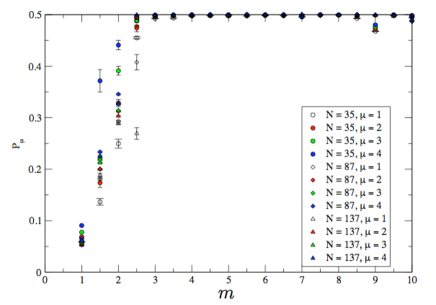
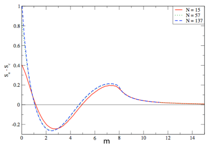
Figure 1: The left panel is a plot of $P_{\mu}$ as a function of $m$ for several different values of $N$. The right panel shows a plot of $S_{u}-S_{c}$ as a function of $m$ for several different values of $N$.

IV Non-perturbative results

We need to verify if the results obtained in one-loop perturbation theory in the previous section remains valid in a full non-perturbative computation. The non-perturbative computation is performed using the Hybrid Monte Carlo algorithm. Let $H_{\mu}$ be traceless Hermitian matrices that are conjugate to the gauge fields, $U_{\mu}$. The algorithm starts with one choice for $U_{\mu}$. Then, we draw $H_{\mu}$ according to a Gaussian distribution.

The equations of motion for $U_{\mu}$ are

$$\frac{dU_{\mu}}{d\tau}=iH_{\mu}U_{\mu}.$$ (22)

Setting $\frac{dS}{d\tau}=0$ results in

$$\sum_{\mu=1}^{4}{\rm Tr}\left[H_{\mu}\frac{dH_{\mu}}{d\tau}\right]+\frac{dS_{g}}{d\tau}+\frac{dS_{f}}{d\tau}=0.$$ (23)

The derivative of $S_{f}$ with respect to $\tau$ is referred to as fermionic force term and is computationally intensive. One can derive exact expressions for the single site model Hietanen:2009ex . It involves exact diagonalization of $H$ and the computational cost grows like $N^{6}$. The advantage of computing the fermionic force exactly is that one can work with any real value of $f$. An alternative approach is to use the pseudo-fermion algorithm to compute the fermionic force term inprep . This is less computationally intensive but works only for integer values of $f$.

The result for massless fermions (we set $\mu=0.01$ in the numerical simulation) is shown in the left panel of Fig. 2 using the exact algorithm for the fermionic force. We can see that the theory will reproduce the correct continuum limit if $m>3$. We set $m=5$ and studied the behavior of the model as a function of the quark mass. The result is plotted in the right panel of Fig. 2. We see that the model will reproduce correct continuum physics even when the fermions are massive.

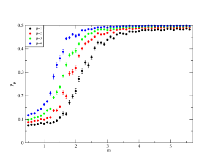
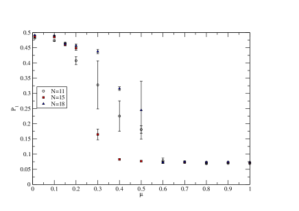
Figure 2: The left panel is a plot of $P_{\mu}$ as a function of $m$ in the full numerical simulation with $N=11$, $b=7$, $f=\frac{1}{2}$ and $\mu=0.01$. The right panel shows a plot of $P_{1}$ (this is the one that is broken first) as a function of $\mu$ for several different values of $N$.

IV.1 Chiral symmetry

In order to study whether chiral symmetry is spontaneously broken, we studied the behavior of the low lying positive eigenvalues, $0<\lambda_{1}<\lambda_{2}\cdots$, of the hermitian overlap Dirac operator. If chiral symmetry is broken, we expect a relation of the form

$$z_{i}=N^{2}\lambda_{i}\Sigma(b)$$ (24)

where the joint distribution of the scaled variables, $z_{i}$, are given by some chiral random matrix model Verbaarschot:2000dy and $\Sigma(b)$ is the value of the chiral condensate.

The chiral Random Matrix theory ensemble for a symplectic matrix, $C=\sum_{\mu}\sigma_{\mu}C_{\mu}$, is

$$Z=\int[dC_{\mu}]e^{-\sum_{\mu}\sum_{ij}\left[C_{\mu}^{ij}\right]^{2}}\left[\det H_{\rm rmt}\right]^{f};\ \ \ \ H_{\rm rmt}=\pmatrix{\mu&C\cr C^{\dagger}&-\mu\cr}$$ (25)

with $C_{\mu}$ being a real square matrix. We expect $z_{i}$ to be the eigenvalues of $H_{\rm rmt}$ with $\Sigma(b)$ being the scale that relates these eigenvalues to the eigenvalues of $H_{o}$. We want to eliminate the scale set by the chiral condensate, and we focus on

$$r=\left\langle\frac{\lambda_{1}}{\lambda_{2}}\right\rangle.$$ (26)

The result as a function of $f$ with $b=5$, $m=5$, $\mu=0.01$ and $N=11$ is shown in the left panel of Fig.3. By comparion with chiral random matrix theory, it looks like chiral symmetry is broken for $f=0$ and $f=1$ but not for $f>1$. This would be the case if the non-pertubative beta function has a zero for $f>1$.

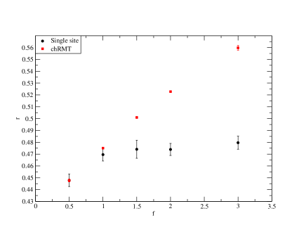
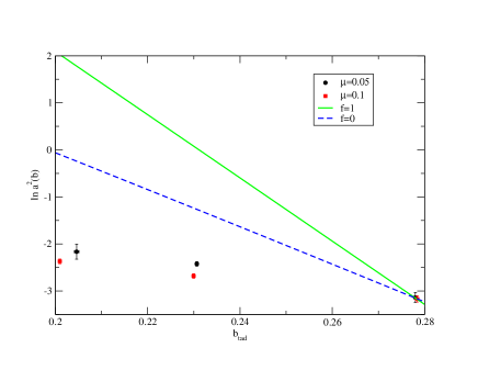
Figure 3: The left panel is a plot of $r$ as a function of $f$ in the full numerical simulation with $N=11$, $b=5$, and $\mu=0.01$. The right panel shows the lattice scale as a function of the lattice coupling for $f=1$. The two loop result for $f=0$ and $f=1$ are shown for comparison.

IV.2 Setting the scale

In order to get some insight into the non-perturbative beta function, we study a lattice scale as a function of the lattice coupling. An $L\times T$ Wilson loop operator in the $\mu-\nu$ plane is given by

$$W(L,T)=U_{\mu}^{L}U_{\nu}^{T}{U_{\mu}^{\dagger}}^{L}{U_{\mu}^{\dagger}}^{T}.$$ (27)

The eigenvalues, $e^{i\theta_{k}}$; $k=1,\cdots,N$ of this operator are gauge invariant. Let $p(\theta;L,T,b)$ be the distribution of these eigenvalues with $\theta\in[-\pi,\pi)$. This distribution undergoes a transition Narayanan:2006rf at $N\to\infty$ as the area, $LT$, is changed at a fixed coupling $b$: the distribution has a gap at $\pi$ for small areas and it becomes gapless for large areas. There is a critical area $A_{c}(b)$ where the gap closes. There is a universal function Narayanan:2007dv describing the distribution in terms of the scaled variables derived from $A(b)$ and $\theta$ in the vicinity of $A_{c}(b)$ and $\pi$.

Let

$$O_{N}(y;A,b)=\langle\det\left(e^{\frac{y}{2}}+e^{-\frac{y}{2}}W(L,T)\right)\rangle;\ \ \ \ A=LT.$$ (28)

The region close to $y=0$ probes $\theta$ close to $\pi$. Let

$$O_{N}(y;A,b)=C_{0}(A,b,N)+C_{1}(A,b,N)y^{2}+C_{2}(A,b,N)y^{4}+\cdots.$$ (29)

It is useful to define

$$\Omega(A,b,N)=\frac{C_{0}(A,b,N)C_{2}(A,b,N}{C_{1}^{2}(A,b,N)}.$$ (30)

One can show using the universal scaling function that

$$\Omega(A_{c}(b),n,\infty)=\frac{\Gamma^{4}\left(\frac{1}{4}\right)}{48\pi^{2}}=0.364739936$$ (31)

We can define $A_{c}(b,N)$ at a fixed $N$ and $b$ as the area where

$$\Omega(A_{c}(b,N),b,N)=0.364739936,$$ (32)

and

$$\lim_{N\to\infty}A_{c}(b,N)=A_{c}(b),$$ (33)

will be the location of the transition at infinite $N$.

Since we are working at a fixed but large $N$ in this paper, we will define our length scale as

$$a(b)=\frac{1}{\sqrt{A_{c}(b,N)}}.$$ (34)

It is necessary to work with a lattice coupling that shows the weak to strong coupling transition that is essentially free of finite $N$ effects. We chose $N=18$ and set the lattice couplings to $b=0.32,0.35,0.4$. The fermion mass was set to $\mu=0.1$ and $\mu=0.05$ and we set $m=4$. The pseudo-fermion algorithm was used to compute the fermionic force.

This is an irrelevant parameter but needs to be chosen in a specific range to realize the correct continuum limit. Based on previous studies Hietanen:2010fx , we set $m=4$ in this paper.

We restrict ourselves to square Wilson loops and this enables us to extract a length scale using linear interpolation. The results are plotted in the right panel of Fig. 3 and compared with the two loop result for $f=0$ and $f=1$. The length scale changes very little in the range of coupling we have studied in this paper. Let us assume a beta function of the form

$$\beta(\alpha)=\epsilon+(\alpha-\alpha_{0})^{2}$$ (35)

motivated by Kaplan:2009kr . Assume $\epsilon>0$ but small for our case since the two loop beta function has a zero if $f$ is slightly bigger than unity. The scale as a function of the coupling is given by

$$\ln a^{2}=\frac{1}{\sqrt{\epsilon}}\tan^{-1}\frac{\alpha-\alpha_{0}}{\sqrt{\epsilon}}.$$ (36)

If $\epsilon$ is small and our lattice coupling is larger than $\alpha_{0}$ and not close to it, the scale will change very little if we change the coupling. This leads us to speculate that the single site model we are simulating might be close to a situation where the beta function has a zero. A careful analysis of the large $N$ corrections along with results at weaker coupling are needed to confirm this speculation. In addition, it will be necessary to study the chiral limit. The effect due to fermion masses in the right panel of Fig. 3 are small.

- (1) L. Del Debbio, PoS LATTICE2010, 004 (2010).
- (2) S. Catterall, L. Del Debbio, J. Giedt, L. Keegan, [arXiv:1108.3794 [hep-ph]].
- (3) T. DeGrand, Y. Shamir, B. Svetitsky, Phys. Rev. D83, 074507 (2011). [arXiv:1102.2843 [hep-lat]].
- (4) A. J. Hietanen, K. Rummukainen, K. Tuominen, Phys. Rev. D80, 094504 (2009). [arXiv:0904.0864 [hep-lat]].
- (5) P. Kovtun, M. Unsal, L. G. Yaffe, JHEP 0706, 019 (2007). [hep-th/0702021 [HEP-TH]].
- (6) T. J. Hollowood and J. C. Myers, arXiv:0907.3665 [hep-th].
- (7) B. Bringoltz, JHEP 0906, 091 (2009). [arXiv:0905.2406 [hep-lat]].
- (8) B. Bringoltz, arXiv:0911.0352 [hep-lat].
- (9) A. Hietanen, R. Narayanan, JHEP 1001, 079 (2010). [arXiv:0911.2449 [hep-lat]].
- (10) T. Azeyanagi, M. Hanada, M. Unsal, R. Yacoby, Phys. Rev. D82, 125013 (2010). [arXiv:1006.0717 [hep-th]].
- (11) A. Hietanen, R. Narayanan, Phys. Lett. B698, 171-174 (2011). [arXiv:1011.2150 [hep-lat]].
- (12) S. Catterall, R. Galvez, M. Unsal, JHEP 1008, 010 (2010). [arXiv:1006.2469 [hep-lat]].
- (13) R. G. Edwards, U. M. Heller, R. Narayanan, Phys. Rev. D59, 094510 (1999). [hep-lat/9811030].
- (14) H. Neuberger, Phys. Lett. B417, 141-144 (1998). [hep-lat/9707022].
- (15) G. Bhanot, U. M. Heller and H. Neuberger, Phys. Lett. B 113, 47 (1982).
- (16) A. Hietanen, R. Narayanan, work in progress.
- (17) J. J. M. Verbaarschot, T. Wettig, Ann. Rev. Nucl. Part. Sci. 50, 343-410 (2000). [hep-ph/0003017].
- (18) R. Narayanan, H. Neuberger, JHEP 0603, 064 (2006). [hep-th/0601210].
- (19) R. Narayanan, H. Neuberger, JHEP 0712, 066 (2007). [arXiv:0711.4551 [hep-th]].
- (20) D. B. Kaplan, J. -W. Lee, D. T. Son, M. A. Stephanov, Phys. Rev. D80, 125005 (2009). [arXiv:0905.4752 [hep-th]].