FPEOS: A First-Principles Equation of State Table of Deuterium for Inertial Confinement Fusion Applications

Abstract

Understanding and designing inertial confinement fusion (ICF) implosions through radiation-hydrodynamics simulations rely on the accurate knowledge of the equation of state (EOS) of the deuterium and tritium fuels. To minimize the drive energy for ignition, the imploding shell of DT-fuel needs to be kept as cold as possible. Such low-adiabat ICF implosions can access to coupled and degenerate plasma conditions, in which the analytical or chemical EOS models become inaccurate. Using the path integral Monte Carlo (PIMC) simulations we have derived a first-principles EOS (FPEOS) table of deuterium that covers typical ICF fuel conditions at densities ranging from 0.002 to 1596 g/cm³ and temperatures of 1.35 eV $-$ 5.5 keV. We report the internal energy and the pressure, and discuss the structure of the plasma in terms of pair correlation functions. When compared with the widely used SESAME table and the revised Kerley03 table, discrepancies in the internal energy and in the pressure are identified for moderately coupled and degenerate plasma conditions. In contrast to the SESAME table, the revised Kerley03 table is in better agreement with our FPEOS results over a wide range of densities and temperatures. Although subtle differences still exist for lower temperatures ($T<10$ eV) and moderate densities ($1-10$ g/cm³), hydrodynamics simulations of cryogenic ICF implosions using the FPEOS table and the Kerley03 table have resulted in similar results for the peak density, areal density $\rho R$, and neutron yield, which are significantly different from the SESAME simulations.

I Introduction

Inertial confinement fusion (ICF) has been pursued for decades since the concept was introduced in 1972 ICF . In the traditional central-hot-spot ignition designs, a capsule of cryogenic deuterium-tritium (DT) covered with plastic ablator is driven to implode either directly by intense laser pulses DDI or indirectly by x-rays in a hohlraum IDI . To minimize the driving energy required for ignition, the imploding DT-capsule needs to be maintained as cold as possible Betti for high compressions (larger than a thousand times that of the solid DT density) at the stagnation stage. This can either be done with fine-tuned shocks GoncharovPRL_2010 or with ramp compression waves. The reduction in temperature leads to pressures in the imploding DT-shell that are just above the Fermi degeneracy pressure. This is conventionally characterized by the so-called adiabat parameter $\alpha=P/P_{F}$. Low-adiabat ICF designs with $1<\alpha<2$ are currently studied with indirect-drive implosions at the National Ignition Facility (NIF) NIF . Direct-drive ignition designs GoncharovPRL_2010 for NIF also place the DT-shell adiabat at a low value of $2<\alpha<3$. Cryogenic DT targets scaled from the hydro-equivalent NIF designs are routinely imploded with a direct drive at the Omega laser facility omega .

Since the compressibility of a material is determined by its equation of state (EOS) Hu_PRL_2008 , the accurate knowledge of the EOS of the DT-fuel is essential for designing ICF ignition targets and predicting the performance of the target during ICF implosions. To perform radiation-hydrodynamics simulations of ICF implosions, one needs to know the pressure and energy of the DT-fuel and the ablator materials at various density and temperature conditions, which are usually provided by EOS tables or analytical formulas. Various EOS tables for deuterium have been assembled because its importance in ICF applications, planetary science and high pressure physics.

The widely used SESAME EOS table of deuterium Kerley1972 ; Kerley2003 was based upon a chemical model for hydrogen SaumonPRA1992 ; Ross1998 ; Rogers2001 ; Juranek2002 that describes the material in terms of well-defined chemical species like H₂ molecules, H atoms and free protons and electrons. Their interaction as well as many-body and degeneracy effects are treated approximately. For the SESAME table, liquid perturbation theory was adopted in the molecular/atomic fluid phase for ICF plasma conditions. A first-order expansion that only takes into account nearest neighbor interactions was used in the original SESAME table Kerley1972 .

Chemical models are expected to work well in the regime of weak coupling. However, in ICF implosions, the DT shell goes through a wide range of densities from 0.1 up to 1000 g/cm³ and temperatures varying from a few electron volts (eV) to several hundreds of electron volts DDI ; IDI , which include plasma conditions with moderately strong coupling. This provides the primary motivation for this paper, where we derive the deuterium from first-principles path integral Monte Carlo simulations PierleoniPRL1994 ; MagroPRL1996 ; MilitzerPRL2000 ; MilitzerPRL2001 .

The conditions for a low-adiabat ($\alpha\simeq 2.5$) cryogenic DT implosion on OMEGA are shown in Fig. 1 on panels (a)-(c). Panels (d)-(f) characterize the conditions for a direct-drive ignition design for NIF that is hydro-equivalent to the OMEGA implosion. In panels (a) and (d), we plot the laser pulse shapes. Panels (b) and (e) show the density, $\rho$, and temperature, $T$, path of the driven DT-shell that we derived with one dimensional (1D) hydro-simulations using the hydro-code LILAC LILAC . The DT shell is predicted to undergo a variety of drive stages including several shocks and the final push by the main pulse.

The $\rho$-$T$ path of the imploding DT shell can be projected onto a plane spanned by the coupling parameter $\Gamma=1/(r_{s}k_{b}T)$ and the degeneracy parameter $\theta=T/T_{F}$. $T_{F}=\frac{\hbar^{2}}{2m_{e}k_{b}}\times(3\pi^{2}n)^{2/3}$ is the Fermi temperature of the electrons in a fully ionized plasma and $r_{s}$ is the Wigner-Seitz radius that is related to the number density of the electrons, $n=3/(4\pi r_{s}^{3})$. One finds that the imploding shells indeed pass through the strongly coupled ($\Gamma>1$) and degenerate ($\theta<1$) regimes and one expects coupling and degeneracy effects to play significant roles in the compression and yield-production in low-adiabat ICF implosions FPEOS_PRL .

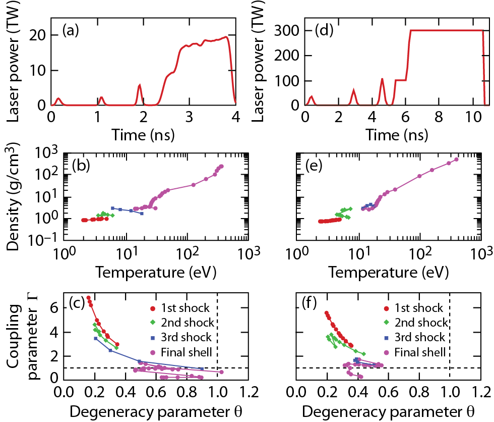
Figure 1: (Color online) (a)-(c): A cryogenic DT-implosion on OMEGA with the triple-picket step-pulse; (d)-(f): A direct-drive ignition design for NIF, scaled from hydro-equivalent OMEGA implosions. In both cases, strongly coupled and degenerated plasma conditions are indeed accessed.

Strong coupling and degeneracy effects in ICF plasmas have recently attracted much attention, as they may redefine the so-called 1D-physics of ICF implosions. The essential pieces of physics models used in ICF hydro-simulations, such as the electron-ion energy relaxation rate relax-rates , the thermal conductivity French_PRL_2008 , the fusion reaction rate Polluk2004 , and viscosity and mutual diffusion in deuterium-tritium mixtures Kress2010 in coupled and degenerated plasmas have been re-examined recently with experimental and theoretical methods. EOS measurements of liquid deuterium along the principal Hugoniot reaching about 100-200 GPa have been performed using laser-driven shock waves Silva1997 ; Collins1998Science ; Collins1998POP ; MostovychPRL ; Boehly2004 ; Hicks2009 , magnetically driven flyers Knudson2001 ; Knudson2004PRB , and convergent explosives Belov2002 ; Fortov2007 . First-principles computer simulations have emerged as the preferred theoretical tool to derive the EOS of deuterium under such extreme conditions. Two methods have been most successful: density functional molecular dynamics (DFT-MD) LACollins1995 ; Lenosky2000 ; GalliPRB2000 ; CollinsPRB2001 ; Clerouin2001 ; DesjarlaisPRB2003 ; BonevPRB2004 and the path integral Monte Carlo (PIMC) PierleoniPRL1994 ; MagroPRL1996 ; MilitzerPRL2000 ; MilitzerPRL2001 . In contrast to chemical models, these first-principles methods can take many-body effects fully into account. Results from such simulations have also been used to revise the original SESAME EOS table of deuterium to yield the improved Kerley03 EOS table Kerley2003 .

For ICF applications, we are especially concerned about the EOS accuracy along the implosion path in the density-temperature plane, i.e., in the range of $\rho=0.1-1000$ g/cm³ and $T=1-1000$ eV. For such high temperatures, standard DFT methods become prohibitively expansive because of the large number of electronic orbitals that would need to be included in the calculation to account for electronic excitations Collins_QMD . Orbital-free semi-classical simulation methods based on Thomas-Fermi theory OFMD is more efficient but they approximate electronic correlation effects and cannot represent chemical bonds. Therefore, in current form, they cannot describe the systems at lower temperatures accurately.

Path integral Monte Carlo has been shown to work rather well for EOS calculations of low-Z materials such as deuterium FPEOS_PRL and helium Mi06 ; Milizer_He_2009 . In this paper we present a first-principles equation of state (FPEOS) table of deuterium from restricted PIMC simulations CeperleyRMP1995 . This method has been successfully applied to compute the deuterium EOS MilitzerPRL2000 ; MiltzerPhD up to a density of $\rho=5.388$ g/cm³. At lower temperatures, the PIMC results have been shown to agree well with DFT-MD calculations for hydrogen MilitzerPRL2001 and more recently for helium Milizer_He_2009 .

Our FPEOS table derived from PIMC covers the whole DT-shell plasma conditions throughout the low-adiabat ICF implosions. Specifically, our table covers densities ranging from 0.002 to $1596$ g cm^-3 and temperatures of 1.35 eV $-$ 5.5 keV. When compared with the widely used SESAME-EOS table and the revised Kerley03-EOS table, discrepancies in the internal energy and the pressure have been identified in moderately coupled and degenerate regimes. Hydrodynamics simulations for cryogenic ICF implosions using our FPEOS table and the Kerley03-EOS table have resulted in similar peak density, areal density $\rho R$, and neutron yield, which differ significantly from the SESAME simulations.

The paper is organized as follows. A brief description of the path integral Monte Carlo method is given in Sec. II. In Sec. III our FPEOS table is presented. In Sec. IV, we characterize the properties of the deuterium plasma for a variety of density and temperature conditions in terms of pair correlation functions. Comparisons between the FPEOS table, the SESAME and the Kerley03 EOS as well as the simple Debye-Hückel plasma model are made in Sec. V. In Sec. VI, we analyze the implications of different EOS tables for ICF applications through hydro-simulations and comparisons with experiments. The paper is summarized in Sec. VII.

II The Path integral Monte Carlo method

Path integral Monte Carlo (PIMC) is the appropriate computational technique for simulating many-body quantum systems at finite temperatures. In PIMC calculations, electrons and ions are treated on equal footing as paths, which means the quantum effects of both species are included consistently, although for the temperatures under consideration, the zero-point motion and exchange effects of the nuclei are negligible.

The fundamental idea of the path integral approach is that the density matrix of a quantum system at temperature, $T$, can be expressed as a convolution of density matrices at a much higher temperature, $M\times T$:

$$\rho({\bf R,R^{\prime}};\beta) = \int d{\bf R}_{1}\,d{\bf R}_{2}\,\cdots\,d{\bf R}_{M-1}\,\rho({\bf R,R}_{1};\Delta\beta)$$ (1)

$$\times \rho({\bf R}_{1},{\bf R}_{2};\Delta\beta)\cdots\rho({\bf R}_{M-1},{\bf R^{\prime}};\Delta\beta).$$

This is an exact expression. The integral on the right can be interpreted as a weighted average over all paths that connect the points ${\bf R}$ and ${\bf R^{\prime}}$. ${\bf R}$ is a collective variable that denote the positions of all particles ${\bf R}=\{{\bf r}_{1},\ldots{\bf r}_{N}\}$. $\beta=1/k_{b}T$ represents length of the path in “imaginary time” and $\Delta\beta=\beta/M$ is the size of each of the $M$ time steps.

From the free particle density matrix which can be used for the high-temperature density-matrices,

$$\rho^{[1]}_{0}({\bf r,r^{\prime}};\beta)=(2\pi\hbar^{2}\beta/m)^{-d/2}\exp\left\{-\frac{({\bf r}-{\bf r}^{\prime})^{2}}{2\hbar^{2}\beta/m}\right\}\;,$$ (2)

one can estimate that the separation of two adjacent positions on the path, $\Delta r={\bf r}_{i+1}-{\bf r}_{i}$ can only be on the order of $\sqrt{\hbar^{2}\Delta\beta/m}$ while the separation of the two end points is approximately $\sqrt{\hbar^{2}\beta/m}$. One can consequently interpret the positions ${\bf R}_{1}\ldots{\bf R}_{M-1}$ as intermediate points on a path from ${\bf R}$ and ${\bf R^{\prime}}$. The multi-dimensional integration over all paths in Eq. 1 can be performed efficiently with Monte Carlo methods CeperleyRMP1995 .

In general observables associated with operator, $\hat{O}$, can be derived from,

$$\left<\hat{O}\right>=\frac{\int{\bf d}{\bf R}\int{\bf d}{\bf R^{\prime}}\left<{\bf R}\right|\hat{O}\left|{\bf R^{\prime}}\right>\rho({\bf R^{\prime}},{\bf R};\beta)}{\int{\bf d}{\bf R}\;\rho({\bf R},{\bf R};\beta)}\;,$$ (3)

but for the kinetic and potential energies, $E_{K}$ and $E_{P}$, as well as for pair correlation functions only diagonal matrix elements (${\bf R}={\bf R}^{\prime}$) are needed. The total internal energy follows from $E=E_{K}+E_{P}$ and the pressure, $P$, can be obtained from the virial theorem for Coulomb systems,

$$P=(2E_{K}+E_{P})/3V\;.$$ (4)

$V$ is the volume.

Electrons are fermions and their fermionic characters matters for the degenerate plasma conditions under consideration. This implies one needs to construct an antisymmetric many-body density matrix, which can be derived by introducing a sum of all permutations, ${\mathcal{P}}$, and then also include paths from ${\bf R}$ to ${\mathcal{P}}{\bf R}^{\prime}$. While this approach works well for bosons CeperleyRMP1995 , for fermions each permutation must be weighted by a factor $(-1)^{\mathcal{P}}$. The partial cancellation of contributions with opposite signs leads to an extremely inefficient algorithm when the combined position and permutation space is sampled directly. This is known as Fermion sign problem, and its severity increases as the plasma becomes more degenerate.

We deal with the Fermion sign problem by introducing the fixed node approximation Ce91 ; Ce96 ,

$$\rho_{F}({\bf R},{\bf R}^{\prime};\beta)=\frac{1}{N!}\;\sum_{\mathcal{P}}\;(-1)^{\mathcal{P}}\!\!\!\!\!\!\!\!\!\!\!\!\!\int\limits_{\begin{array}[]{c}\scriptstyle{\bf R}\rightarrow{\mathcal{P}}{\bf R}^{\prime}\\[-2.84526pt] \scriptstyle\rho_{\scriptscriptstyle T}({\bf R},{\bf R}_{t};t)>0\end{array}}\!\!\!\!\!\!\!\!\!\!\!\!\!{\bf d}{\bf R}_{t}\;\;e^{-S[{\bf R}_{t}]},$$ (5)

where one only includes those paths that satisfy the nodal constraint, $\rho_{T}({\bf R},{\bf R}_{t};t)>0$, at every point. $S[{\bf R}_{t}]$ is the action of the path and $\rho_{T}$ is a fermionic trial density a matrix that must be given in analytic form. For this paper, we rely on free particle nodes,

$$\rho_{T}({\bf R},{\bf R^{\prime}};\beta)=\left|\begin{array}[]{ccc}\rho^{[1]}({\bf r}_{1},{\bf r}^{\prime}_{1};\beta)&\ldots&\rho^{[1]}({\bf r}_{N},{\bf r}^{\prime}_{1};\beta)\\ \ldots&\ldots&\ldots\\ \rho^{[1]}({\bf r}_{1},{\bf r}^{\prime}_{N};\beta)&\ldots&\rho^{[1]}({\bf r}_{N},{\bf r}^{\prime}_{N};\beta)\end{array}\right|.$$ (6)

but the nodes of a variational density matrix MP00 have also been employed in PIMC computations MilitzerPRL2000 ; Mi06 ; Milizer_He_2009 .

We have performed a number of convergence tests to minimize errors from using a finite time step and from a finite number of particles in cubic simulation cells with periodic boundary conditions. We determined a time step of $\Delta\beta\leq\left[100\times k_{b}T_{F}\right]^{-1}$ was sufficient to accurately account for all interactions and degeneracy effects. We perform our PIMC calculations with different numbers of atoms depending on the deuterium density: $N=64$ atoms for $\rho<2.5$ g cm^-3, $N=128$ atoms for $2.5<\rho<10.5$ g cm^-3. and $N=256$ atoms for $\rho>10.5$ g cm^-3.

III The FPEOS table of deuterium

We have carried out PIMC calculations for a variety of density and temperature conditions that are of interests to inertial confinement fusion applications. The resulting FPEOS table for deuterium covers the density range from 0.0019636 g cm^-3 ($r_{s}=14$ in units of Bohr radii $a_{0}$) to 1596.48802 g cm^-3 ($r_{s}=0.15$ $a_{0}$) and the temperature interval from 15 625 K ($\simeq 1.35$ eV) to $6.4\times 10^{7}$ K ($\simeq 5515.09$ eV). Fig. 2 shows the conditions for every simulation combined with lines for $\Gamma=1$ and $\theta=1$ to indicate the boundaries between coupled/uncoupled and degenerate/non-degenerate plasma conditions. Plasma conditions in the upper left corner of the diagram are weakly coupled and classical ($\Gamma\ll 1$ and $\theta\gg 1$), while the lower right of the diagram represent strongly coupled and highly degenerate conditions ($\Gamma\gg 1$ and $\theta\ll 1$). The lowest temperatures in our PIMC calculations reach to the regime of $\theta\simeq 0.1$.

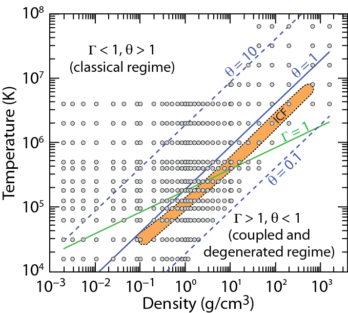
Figure 2: (Color online) The temperature and density conditions covered by the FPEOS table. The gray circles represent our PIMC calculations, while the shell conditions in ICF implosions are schematically shown by the region in orange color. The blue and green lines of $\theta=1$ and $\Gamma=1$ characterize the boundaries of degeneracy and coupling conditions, respectively.

To give an example for the ICF plasma conditions, we added the conditions of an imploding DT capsule shown in Fig. 1 to Fig. 2. It can be seen that the DT shell undergoes a change from strongly coupled to an uncoupled regime during the shock transits. The electronic conditions change from fully degenerated to partially degenerate accordingly. All these conditions are covered by our PIMC results that we have assembled into the following FPEOS table 1. The pressure and the internal energy as well as their statistical error bars from PIMC simulations are listed for different density and temperature conditions.

Table 1: FPEOS table with pressures and internal energy per atom for deuterium. The statistical uncertainties from the PIMC simulations are in given in brackets e.g. 0.219(5)=0.219$\pm$0.005, 414.4(1.6)=414.4$\pm$1.6, or 70230(400)=70230$\pm$400.

Temperature	Pressure	Internal energy
(K)	(Mbar)	(eV$/$atom)
$\rho$ = 1.96360$\times 10^{-3}$g cm-3 [$r_{s}=14.0$ $a_{0}$]
15625	0.001290(8)	-10.83(3)
31250	0.003364(8)	-2.867(16)
62500	0.009046(8)	11.930(13)
95250	0.014640(8)	21.870(12)
125000	0.019600(10)	30.080(15)
181825	0.028920(8)	45.190(13)
250000	0.040040(12)	63.04(2)
400000	0.06440(2)	102.00(4)
500000	0.08074(2)	128.10(4)
1000000	0.16170(3)	257.30(6)
2000000	0.32390(6)	515.90(10)
4000000	0.64830(14)	1033.0(2)
$\rho$ = 3.11810$\times 10^{-3}$g cm-3 [$r_{s}=12.0$ $a_{0}$]
15625	0.002048(14)	-10.97(3)
31250	0.005105(14)	-3.82(2)
62500	0.013980(12)	10.860(12)
95250	0.022970(11)	21.180(12)
125000	0.030840(15)	29.490(15)
181825	0.045690(13)	44.720(13)
250000	0.063400(19)	62.67(2)
400000	0.10220(4)	101.80(4)
500000	0.12790(3)	127.70(4)
1000000	0.25670(5)	257.10(5)
2000000	0.51440(10)	516.00(10)
4000000	1.0290(2)	1033.0(2)
$\rho$ = 5.38815$\times 10^{-3}$g cm-3 [$r_{s}=10.0$ $a_{0}$]
15625	0.00349(2)	-11.280(20)
31250	0.00845(2)	-4.841(18)
62500	0.02325(2)	9.401(14)
95250	0.038870(19)	20.080(12)
125000	0.05264(3)	28.620(16)
181825	0.07841(2)	44.040(13)
250000	0.10900(3)	62.090(19)
400000	0.17630(7)	101.40(4)
500000	0.22080(7)	127.30(4)
1000000	0.44360(9)	257.00(5)
2000000	0.88830(19)	515.50(11)
4000000	1.7780(4)	1033.0(2)
$\rho$ = 1.05237$\times 10^{-2}$g cm-3 [$r_{s}=8.0$ $a_{0}$]
15625	0.00659(5)	-11.550(17)
31250	0.01580(6)	-5.860(20)
62500	0.04325(4)	7.477(13)
95250	0.07371(4)	18.450(12)
125000	0.10080(5)	27.220(16)
181825	0.15150(4)	42.940(13)
250000	0.21160(7)	61.18(2)
400000	0.34300(13)	100.60(4)
500000	0.43010(13)	126.70(4)
1000000	0.86550(19)	256.50(6)
2000000	1.7350(4)	515.40(11)
4000000	3.4740(8)	1033.0(2)

Table 2: TABLE I. (Continued.)

Temperature	Pressure	Internal energy
(K)	(Mbar)	(eV$/$atom)
$\rho$ = 2.49451$\times 10^{-2}$g cm-3 [$r_{s}=6.0$ $a_{0}$]
15625	0.01485(12)	-11.820(17)
31250	0.03556(11)	-6.948(13)
62500	0.09550(10)	4.773(12)
95250	0.16610(10)	15.740(13)
125000	0.23050(11)	24.790(14)
181825	0.35170(12)	40.920(16)
250000	0.4946(2)	59.40(3)
400000	0.8072(4)	99.19(5)
500000	1.0150(3)	125.40(4)
1000000	2.0480(5)	255.50(6)
2000000	4.1090(9)	514.50(12)
4000000	8.2310(17)	1032.0(2)
$\rho$ = 4.31052$\times 10^{-2}$g cm-3 [$r_{s}=5.0$ $a_{0}$]
15625	0.02537(20)	-11.970(16)
31250	0.05980(19)	-7.537(14)
62500	0.15800(16)	3.087(12)
95250	0.27800(18)	13.820(13)
125000	0.3880(3)	22.910(18)
181825	0.5976(2)	39.250(17)
250000	0.8460(3)	58.01(3)
400000	1.3870(4)	97.96(3)
500000	1.7460(5)	124.40(4)
1000000	3.5310(8)	254.50(6)
2000000	7.0960(13)	513.80(10)
4000000	14.220(3)	1031.0(2)
$\rho$ = 8.41898$\times 10^{-2}$g cm-3 [$r_{s}=4.0$ $a_{0}$]
15625	0.0479(7)	-12.21(2)
31250	0.1150(5)	-8.135(19)
62500	0.2950(6)	1.17(2)
95250	0.5200(6)	11.37(2)
125000	0.7308(7)	20.29(3)
181825	1.1400(6)	36.80(2)
250000	1.6250(9)	55.71(3)
400000	2.6850(11)	96.11(4)
500000	3.3910(11)	122.70(4)
1000000	6.8810(15)	253.30(6)
2000000	13.850(3)	513.00(11)
4000000	27.750(6)	1030.0(2)
$\rho$ = 0.1 g cm-3 [$r_{s}\simeq 3.777$ $a_{0}$]
15625	0.0578(15)	-12.21(5)
31250	0.1351(6)	-8.351(19)
62500	0.3491(6)	0.74(2)
95250	0.6110(6)	10.690(18)
125000	0.8598(8)	19.57(2)
181825	1.3450(9)	36.08(3)
250000	1.9200(9)	55.00(3)
400000	3.1850(13)	95.67(4)
500000	4.0180(11)	122.10(3)
1000000	8.1680(17)	252.90(5)
2000000	16.440(3)	512.40(11)
4000000	32.970(7)	1030.0(2)

Table 3: TABLE I. (Continued.)

Temperature	Pressure	Internal energy
(K)	(Mbar)	(eV$/$atom)
$\rho$ = 0.199561 g cm-3 [$r_{s}=3.0$ $a_{0}$]
15625	0.124(3)	-12.31(4)
31250	0.2740(17)	-8.91(3)
62500	0.6730(17)	-1.11(3)
95250	1.1760(16)	8.14(3)
125000	1.656(2)	16.66(3)
181825	2.6060(15)	32.91(2)
250000	3.753(2)	51.98(3)
400000	6.273(3)	92.85(4)
500000	7.943(2)	119.60(4)
1000000	16.250(5)	251.10(8)
2000000	32.760(7)	510.90(11)
4000000	65.740(14)	1029.0(2)
$\rho$ = 0.306563 g cm-3 [$r_{s}=2.6$ $a_{0}$]
15625	0.219(5)	-12.29(5)
31250	0.447(4)	-9.15(4)
62500	1.048(4)	-1.90(4)
95250	1.781(5)	6.68(5)
125000	2.509(4)	14.98(4)
181825	3.947(3)	30.97(4)
250000	5.693(5)	49.91(5)
400000	9.558(8)	90.87(8)
500000	12.120(6)	117.70(6)
1000000	24.890(9)	249.60(9)
2000000	50.250(13)	509.70(13)
4000000	101.100(19)	1030.0(2)
$\rho$ = 0.389768 g cm-3 [$r_{s}=2.4$ $a_{0}$]
15625	0.298(12)	-12.30(10)
31250	0.597(9)	-9.21(7)
62500	1.337(8)	-2.40(7)
95250	2.280(7)	6.11(6)
125000	3.175(8)	14.09(7)
181825	4.979(11)	29.84(9)
250000	7.206(9)	48.84(7)
400000	12.090(12)	89.61(9)
500000	15.370(14)	116.70(11)
1000000	31.580(14)	248.60(11)
2000000	63.96(2)	509.80(19)
4000000	128.40(3)	1028.0(3)
$\rho$ = 0.506024 g cm-3 [$r_{s}=2.2$ $a_{0}$]
15625	0.42(3)	-12.1(2)
31250	0.849(14)	-9.16(9)
62500	1.789(12)	-2.68(7)
95250	2.954(10)	5.30(6)
125000	4.088(12)	13.02(7)
181825	6.396(10)	28.48(6)
250000	9.243(12)	47.20(7)
400000	15.620(14)	88.25(9)
500000	19.84(3)	115.10(18)
1000000	40.94(3)	247.5(2)
2000000	82.93(3)	508.6(2)
4000000	166.50(4)	1026.0(3)

Table 4: TABLE I. (Continued.)

Temperature	Pressure	Internal energy
(K)	(Mbar)	(eV$/$atom)
$\rho$ = 0.673518 g cm-3 [$r_{s}=2.0$ $a_{0}$]
15625	0.59(4)	-12.02(18)
31250	1.28(2)	-8.96(11)
62500	2.461(10)	-3.01(5)
95250	3.930(7)	4.43(3)
125000	5.413(6)	11.91(3)
181825	8.446(8)	27.08(4)
250000	12.200(7)	45.63(3)
400000	20.660(14)	86.64(6)
500000	26.270(15)	113.50(7)
1000000	54.300(20)	245.90(9)
2000000	110.20(3)	507.20(16)
4000000	221.60(6)	1026.0(3)
$\rho$ = 0.837338 g cm-3 [$r_{s}=1.86$ $a_{0}$]
15625	0.97(6)	-11.3(2)
31250	1.71(2)	-8.85(8)
62500	3.17(4)	-3.17(14)
95250	5.04(4)	4.30(14)
125000	6.80(3)	11.43(11)
181825	10.52(2)	26.29(9)
250000	15.15(3)	44.67(10)
400000	25.62(4)	85.52(16)
500000	32.67(4)	112.70(17)
1000000	67.44(6)	244.9(2)
2000000	136.90(11)	506.2(4)
4000000	275.50(8)	1026.0(3)
$\rho$ = 1.0 g cm-3 [$r_{s}=1.753$ $a_{0}$]
15625	1.33(7)	-11.0(2)
31250	2.22(4)	-8.67(12)
62500	3.92(4)	-3.23(14)
95250	6.06(4)	3.88(13)
125000	8.16(4)	10.90(11)
181825	12.57(3)	25.60(10)
250000	18.07(3)	43.85(10)
400000	30.36(3)	84.00(9)
500000	38.81(3)	111.30(10)
1000000	80.40(4)	243.90(13)
2000000	163.20(6)	505.00(17)
4000000	328.80(8)	1024.0(3)
$\rho$ = 1.00537 g cm-3 [$r_{s}=1.750$ $a_{0}$]
15625	1.35(9)	-10.9(3)
31250	2.23(3)	-8.69(10)
62500	4.03(4)	-2.97(14)
95250	6.03(5)	3.67(16)
125000	8.27(5)	11.09(14)
181825	12.63(3)	25.56(9)
250000	18.17(4)	43.82(13)
400000	30.54(5)	84.05(16)
500000	38.99(8)	111.2(3)
1000000	80.80(7)	243.7(2)
2000000	164.20(11)	505.3(3)
4000000	330.50(12)	1024.0(4)

Table 5: TABLE I. (Continued.)

Temperature	Pressure	Internal energy
(K)	(Mbar)	(eV$/$atom)
$\rho$ = 1.15688 g cm-3 [$r_{s}=1.67$ $a_{0}$]
15625	1.67(11)	-10.9(3)
31250	2.78(5)	-8.35(14)
62500	4.82(6)	-2.87(16)
95250	7.05(6)	3.49(17)
125000	9.65(6)	10.93(17)
181825	14.45(6)	24.77(17)
250000	20.81(5)	42.94(14)
400000	35.12(5)	83.36(13)
500000	44.82(3)	110.50(9)
1000000	92.99(5)	243.30(13)
2000000	189.00(11)	505.0(3)
4000000	380.30(16)	1024.0(4)
$\rho$ = 1.31547 g cm-3 [$r_{s}=1.60$ $a_{0}$]
31250	3.46(9)	-7.9(2)
62500	5.65(10)	-2.8(2)
95250	8.31(8)	3.75(19)
125000	10.97(6)	10.44(15)
181850	16.66(6)	24.76(14)
250000	23.73(5)	42.50(12)
400000	39.92(7)	82.72(17)
500000	50.66(7)	109.20(17)
1000000	105.50(8)	242.30(20)
2000000	214.20(7)	502.90(16)
4000000	431.80(11)	1022.0(3)
$\rho$ = 1.59649 g cm-3 [$r_{s}=1.50$ $a_{0}$]
31250	4.67(13)	-7.5(3)
62500	7.24(12)	-2.7(2)
95250	10.53(13)	3.9(2)
125000	13.68(11)	10.4(2)
181850	20.19(7)	23.87(13)
250000	28.78(8)	41.57(15)
400000	48.31(7)	81.53(14)
500000	61.33(10)	107.90(19)
1000000	128.20(11)	241.8(2)
2000000	260.40(15)	503.1(3)
4000000	524.30(13)	1022.0(3)
$\rho$ = 1.96361 g cm-3 [$r_{s}=1.40$ $a_{0}$]
31250	6.4(2)	-7.0(4)
62500	9.69(15)	-2.1(2)
95250	13.66(14)	4.3(2)
125000	17.11(10)	10.05(16)
181850	25.29(6)	23.68(9)
250000	35.66(9)	41.00(14)
400000	59.23(9)	80.18(15)
500000	75.41(10)	106.90(15)
1000000	156.80(9)	239.50(15)
2000000	319.49(16)	501.2(3)
4000000	644.54(18)	1021.0(3)

Table 6: TABLE I. (Continued.)

Temperature	Pressure	Internal energy
(K)	(Mbar)	(eV$/$atom)
$\rho$ = 2.45250 g cm-3 [$r_{s}=1.30$ $a_{0}$]
62500	12.61(17)	-2.2(2)
95250	18.18(16)	4.9(2)
125000	22.09(15)	10.05(19)
181850	32.63(10)	24.00(13)
250000	45.03(12)	40.55(15)
400000	74.54(10)	79.73(13)
500000	93.88(11)	105.30(14)
1000000	195.60(17)	238.1(2)
2000000	398.20(18)	499.4(2)
4000000	804.2(3)	1020.0(4)
$\rho$ = 3.11814 g cm-3 [$r_{s}=1.20$ $a_{0}$]
62500	18.0(4)	-1.4(4)
95250	24.6(3)	5.4(4)
125000	30.1(5)	11.0(5)
181850	43.0(3)	24.4(4)
250000	57.8(4)	39.9(4)
400000	94.9(2)	78.5(2)
500000	120.10(14)	104.70(14)
1000000	248.4(2)	236.7(3)
2000000	504.5(6)	496.7(6)
4000000	1021.0(5)	1018.0(5)
$\rho$ = 4.04819 g cm-3 [$r_{s}=1.10$ $a_{0}$]
62500	26.2(1.1)	-0.1(8)
95250	34.4(5)	6.1(4)
125000	41.9(6)	12.1(5)
181850	58.8(6)	25.3(5)
250000	75.8(4)	39.0(3)
400000	125.1(3)	78.5(2)
500000	156.8(2)	103.80(16)
1000000	321.0(3)	234.0(3)
2000000	651.5(7)	492.9(5)
4000000	1327.0(8)	1018.0(6)
$\rho$ = 5.38815 g cm-3 [$r_{s}=1.00$ $a_{0}$]
95250	51.9(1.6)	8.3(9)
125000	61.1(8)	13.7(5)
181850	81.8(1.2)	25.9(7)
250000	105.4(8)	40.0(5)
400000	169.1(1.3)	78.2(7)
500000	212.2(1.3)	104.1(8)
1000000	429.4(1.1)	233.5(6)
2000000	867.4(1.2)	491.5(7)
4000000	1768.0(1.0)	1018.0(6)
$\rho$ = 7.39115 g cm-3 [$r_{s}=0.90$ $a_{0}$]
95250	80(2)	10.3(9)
125000	92(2)	15.5(9)
181850	120(2)	27.4(1.0)
250000	153.4(1.3)	41.9(6)
400000	236.6(1.5)	78.2(6)
500000	297.2(1.2)	104.5(5)
1000000	590.2(1.4)	231.8(6)
2000000	1183.0(1.6)	486.5(7)
4000000	2422.0(1.6)	1015.0(7)

Table 7: TABLE I. (Continued.)

Temperature	Pressure	Internal energy
(K)	(Mbar)	(eV$/$atom)
$\rho$ = 10.0000 g cm-3 [$r_{s}\simeq 0.81373$ $a_{0}$]
125000	142(3)	19.0(8)
181850	182(2)	31.8(7)
250000	225.7(1.7)	44.5(5)
400000	334(4)	80.5(1.3)
500000	414.4(1.6)	106.2(5)
1000000	802(2)	230.5(6)
2000000	1596.0(1.6)	483.3(5)
4000000	3276.0(1.6)	1013.0(5)
8000000	6592(3)	2054.0(8)
$\rho$ = 10.5237 g cm-3 [$r_{s}=0.80$ $a_{0}$]
125000	153(7)	19.8(2.0)
181850	197(4)	33.1(1.0)
250000	242(3)	45.4(9)
400000	353(4)	80.4(1.2)
500000	434(4)	105.3(1.1)
1000000	846(3)	231.0(8)
2000000	1681(2)	483.2(7)
4000000	3447(6)	1011.0(1.8)
8000000	6929(3)	2051.0(9)
$\rho$ = 15.7089 g cm-3 [$r_{s}=0.70$ $a_{0}$]
181850	346(9)	40.0(1.7)
250000	419(9)	55.0(1.8)
400000	575(4)	87.1(8)
500000	684(3)	109.3(6)
1000000	1293(4)	233.5(7)
2000000	2515(4)	481.4(9)
4000000	5149(5)	1011.0(1.1)
8000000	10390(5)	2060.0(1.1)
$\rho$ = 24.9451 g cm-3 [$r_{s}=0.60$ $a_{0}$]
400000	1037(12)	98.4(1.4)
500000	1208(17)	121(2)
1000000	2133(11)	239.2(1.4)
2000000	4025(9)	480.9(1.1)
4000000	8195(16)	1009.0(2.0)
8000000	16200(17)	2020(2)
16000000	32950(13)	4124.0(1.6)
$\rho$ = 43.1052 g cm-3 [$r_{s}=0.50$ $a_{0}$]
400000	2212(30)	123(2)
500000	2523(20)	146.5(1.8)
1000000	4002(30)	256.4(2.0)
2000000	7162(18)	490.2(1.3)
4000000	14180(17)	1006.0(1.3)
8000000	28390(30)	2044(2)
16000000	56880(20)	4118.0(1.7)
32000000	114000(40)	8273(3)
64000000	227900(90)	16540(7)
$\rho$ = 84.1898 g cm-3 [$r_{s}=0.40$ $a_{0}$]
1000000	9169(50)	298.4(2.0)
2000000	14950(80)	517(3)
4000000	27960(70)	1007(3)
8000000	54980(40)	2019.0(1.4)
16000000	110600(70)	4093(3)
32000000	222600(120)	8262(4)
64000000	445900(110)	16570(4)

Table 8: TABLE I. (Continued.)

Temperature	Pressure	Internal-energy
(K)	(Mbar)	(eV$/$atom)
$\rho$ = 199.561 g cm-3 [$r_{s}=0.30$ $a_{0}$]
2000000	41350(800)	597(12)
4000000	70230(400)	1056(6)
8000000	129900(500)	2000(8)
16000000	263400(300)	4104(5)
32000000	527000(400)	8247(7)
64000000	1049000(400)	16450(7)
$\rho$ = 673.518 g cm-3 [$r_{s}=0.20$ $a_{0}$]
4000000	299900(4000)	1322(16)
8000000	504200(3000)	2281(15)
16000000	897500(1300)	4121(6)
32000000	1783000(1700)	8251(8)
64000000	3569000(1600)	16560(7)
$\rho$ = 1596.49 g cm-3 [$r_{s}=0.15$ $a_{0}$]
4000000	1071000(20000)	2002(40)
8000000	1555000(20000)	2961(40)
16000000	2342000(17000)	4517(30)
32000000	4565000(16000)	8890(30)
64000000	8523000(8000)	16670(17)

IV Particle Correlations

The correlation functions, $g(r)$, between different pairs of particles such as electron-electron, electron-ion, and ion-ion are particularly interesting for analyzing the physical and chemical changes in the plasma at various density and temperature conditions. The $g(r)$ are available directly in PIMC simulations. We first show the density effects on the structure of the fluid structure by showing how the $g(r)$ functions change with density for three temperatures of 15 625 K, $2.5\times 10^{5}$ K, and $2\times 10^{6}$ K in Figs. 3-5.

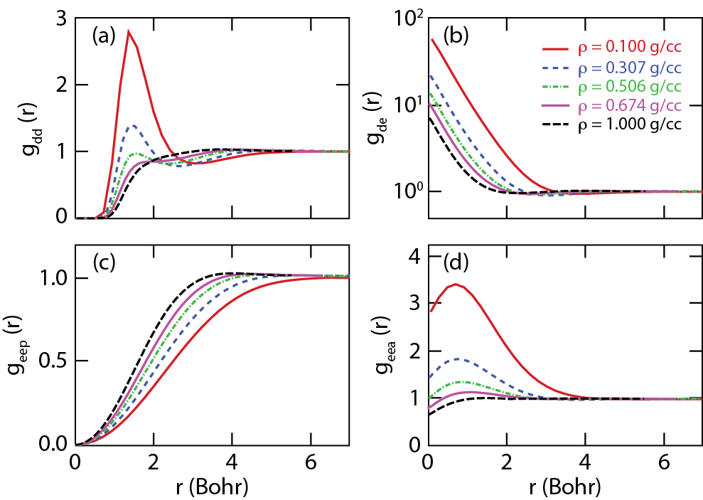
Figure 3: (Color online) The pair correlation functions $g(r)$ derived from PIMC calculations: (a) the ion-ion correlation $g_{dd}(r)$; (b) the ion-electron correlation $g_{de}(r)$; (c) the electron-electron correlation $g_{eep}(r)$ for parallel spins; (d) the electron-electron correlation $g_{eea}(r)$ for anti-parallel spins, with different densities at 15 625 K.

Fig. 3(a) shows a clear peak in the ion-ion correlation function, $g_{dd}(r)$, for 0.1 g/cm³ at the molecular bond length of 1.4 $a_{0}$. As the density of deuterium increases to 1.0 g/cm³, one observes a drastic reduction in peak height which demonstrates the pressure-induced dissociation of D₂ molecules, confirming earlier PIMC results Mi99 ; MiltzerPhD . This interpretation is also supported by the reduction of peak at $r=0$ in the $g_{de}(r)$ function in Fig. 3(b). Furthermore the positive correlation between pair of electrons with anti-parallel spin in Fig. 3(d) is also disappearing with increasing density since they are no longer bound into molecules. Fig. 3(c) shows that there is always a strong repulsion between electrons with parallel spins because of the Pauli exclusion principle but they approach each other more at higher densities.

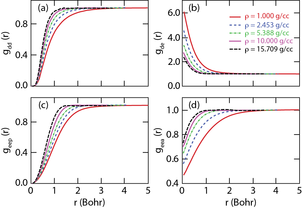
Figure 4: (Color online) Pair correlation functions similar to Fig. 3 but at a higher temperature of $2.5\times 10^{5}$ K and densities from 1.0 to 15.709 g/cm³.

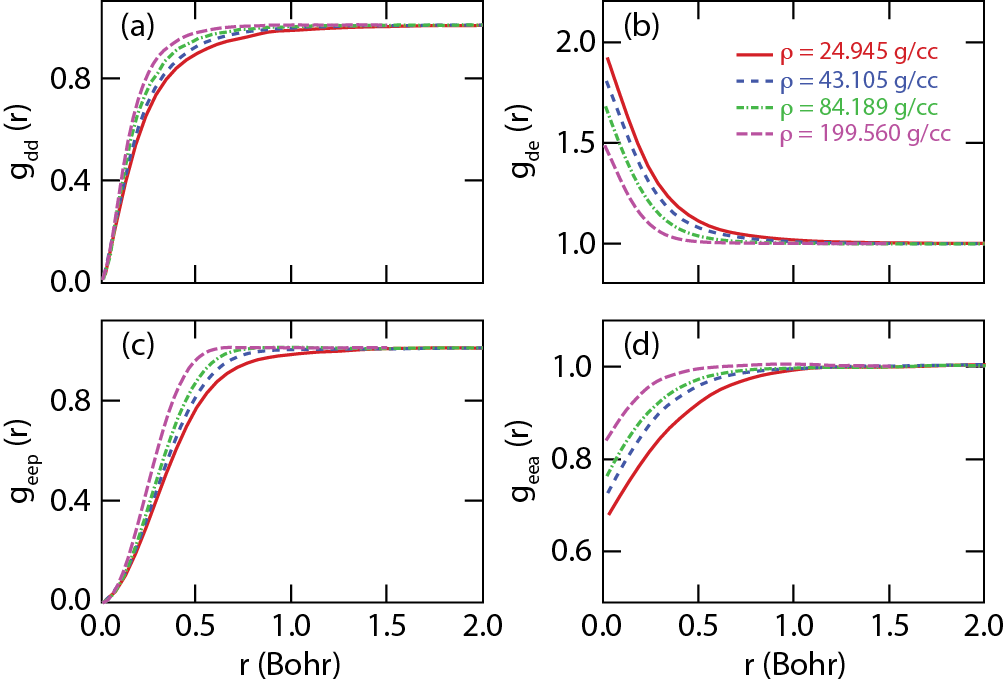
Figure 5: (Color online) Pair correlation functions similar to Fig. 3 but at a higher temperature of $2\times 10^{6}$ K and densities from 24.945 to 199.56 g/cm³.

Figs. 4 and  5 show the pair correlation functions for different densities at much higher temperatures of $2.5\times 10^{5}$ K and $2\times 10^{6}$ K. At these temperatures, $D_{2}$ molecules have completely dissociated as indicated by the absence of the peak in the ion-ion correlation function. The attractive forces between pair of ions have disappeared and repulsion now dominates their interactions. At higher densities, particles are “packed” more tightly and approach each other significantly more so that the $g(r)$ rise up more steeply and reach the values of 0.5 as much smaller distances.

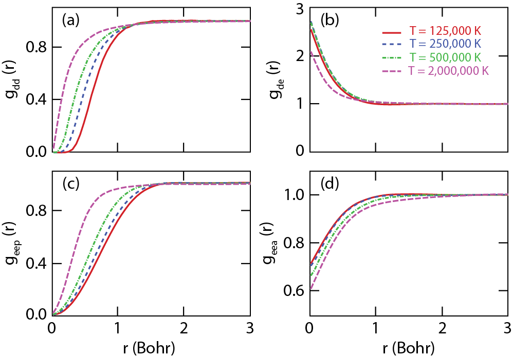
Figure 6: (Color online) Pair correlation functions similar to Fig. 3 at a fixed density of 10.0 g/cm³ for temperatures ranging from $1.25\times 10^{5}$ K to $2\times 10^{6}$ K.

In Fig. 6, we compare the pair correlation functions for the fixed density of 10 g/cm³ for temperatures ranging from $1.25\times 10^{5}$ K to $2\times 10^{6}$ K. It is interesting to note there is relatively little variation between the three curves below the Fermi temperature of $T_{F}=8.8\times 10^{5}$ K but they differ significantly at $2\times 10^{6}$ K. This is a manifestation of Fermi degeneracy effects in which the electrons approach the ground state for temperatures well below the Fermi temperature. Then much of the temperature dependence of the pair correlation functions disappears. For example the pair correlation functions of electrons with anti-parallel spins are almost identical for the two lowest temperatures of $1.25\times 10^{5}$ K and $2.5\times 10^{5}$ K but they differ substantially from results at well above $T_{F}$. When the temperature raises above $T_{F}$, Pauli exclusion effects are reduced, the electrons start to occupy a variety of states, which then has a positive feedback on the mobility of the ions.

V Comparisons of the FPEOS table with SESAME and Kerley03 models

In this section, we compare the pressures and internal energies in our FPEOS table with predictions from the well-known semi-analytical SESAME and Kerley03 EOS tables. To illustrate how much the system deviates from an ideal plasma, we have normalized both pressure and energy to their corresponding values [$E_{id}$ and $P_{id}$] of non-interacting gas of classical ions and fermionic electrons. This removes most of the temperature dependence and emphasizes the effects of the Coulomb interaction, which leads to a reduction in pressure and energy below the non-interacting values in all cases.

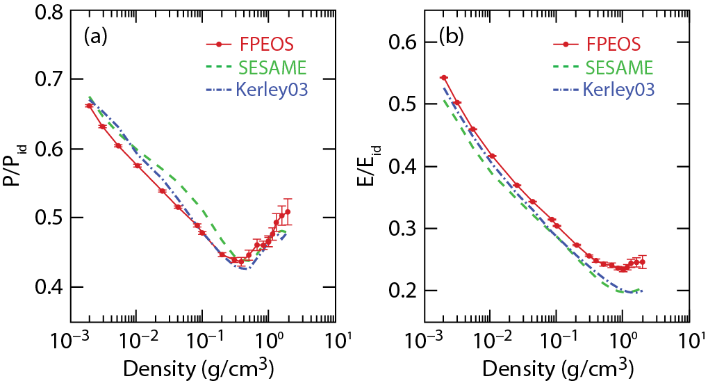
Figure 7: (Color online) The comparisons of pressure (a) and internal energy (b) as a function of density from the the FPEOS, SESAME, Kerley03 tables. The error bars indicate the 1$\sigma$ statistical uncertainty in the PIMC simulations. Results were normalized to non-interacting gas of classical ions and fermionic electrons.

In Figs. 7$-$9, we plot the pressure and the internal energy as a function of density for different temperatures ranging from $31250$ to $4\times 10^{6}$ K. Figs. 10$-$13 show them as function of temperature for different densities varying between 0.1 and 84.19 g/cm³.

In Fig. 7, we compare FPEOS, SESAME, and Kerley03 results at a comparatively low temperature of 31250 K. This is difficult regime to describe by chemical models because the plasma consists of neutral species like molecules and atoms as well as charged particles such as ions and free electrons. The interaction between neutral and charged species is very difficult analytically while it poses no major challenge to first-principles simulations. As is shown by Fig. 7(a), the SESAME EOS predicts overall higher pressures at low density ($\rho\leq 0.3$ g/cm³) but then all three models come to agree with each other at higher densities. The improved Kerley03 table still showed some discrepancy at very low densities, even though some improvements to the ionization equilibrium model have been made Kerley2003 .

Fig. 7(b) shows that the internal energies predicted by SESAME and Kerley03 are overall lower than the FPEOS values. The higher the density, the more discrepancy there is. Again, this manifests the difficulty of chemical models at such plasma conditions.

One expects the pressure and internal energy to approach the values of a non-interacting gas in the low-density and the high-density limit. At low density, particles are so far away from each other that the interaction effects become negligible. At high density, Pauli exclusion effects dominate over all other interactions and all thermodynamic function can be obtained from the ideal Fermi gas. Just at an intermediate density range which still spans several orders of magnitude, the Coulomb interaction matters and significant deviations for the ideal behavior are observed.

For a higher temperature of $2.5\times 10^{5}$ K, the pressure and energy are compared in Fig. 8. The low-density deuterium at this temperature becomes fully ionized and can therefore be described by the Debye-Hückel plasma model DH-model , which is based on the self-consistent solution of the Poisson equation for a system of screened charges. The pressure and energy per particle (counting electrons and ions) can be explicitly expressed as:

$$P_{D}=P_{id}-\frac{k_{b}T}{24\pi\lambda_{D}^{3}}\;\;{\rm and}\;\;E_{D}=E_{id}-\frac{k_{b}T}{8\pi n\lambda_{D}^{3}}~{},$$ (7)

with the particle number density $n$, the Boltzmann constant $k_{b}$, and the Debye length $\lambda_{D}=\sqrt{k_{b}T/4\pi ne^{2}}$.

We have added the Debye-Hückel results to Figs. 8-13. In Fig. 8 one finds that the simple Debye-Hückel model perfectly agrees with our PIMC calculations in the lower densities up to 0.1 g/cm³, where the improved Kerley03 EOS also gives very similar pressures and energies. On the other hand, the SESAME EOS overestimates both pressure and energy even at such low densities.

Fig. 8(a) exposes an artificial cusp in pressure in Kerley03 EOS at densities of $1.5-4$ g/cm³ while the internal energy curve is smooth. This artificial pressure cusp appears for all temperatures at roughly the same density and may be related to the artificial double compression peaks in the principal Hugoniot predicted by Kerley03 EOS Kerley2003 . The Debye-Hückel model fails at densities higher than 0.2 g/cm³ for this temperature. It is only applicable to weakly interacting plasmas but otherwise predicts unphysically low pressures and energies.

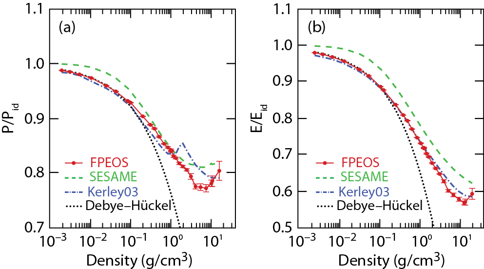
Figure 8: (Color online) Same as Fig. 7 but for a different temperature $2.5\times 10^{5}$ K. The Debye-Hückel model is also shown for comparison.

As the temperature increased to $4\times 10^{6}$ K, the Debye-Hückel model agrees very well with FPEOS in both pressure and energy over a wide range of densities up to 20 g/cm³ as shown in Fig. 9. Significant differences in both pressure and energy are again found for the SESAME EOS, when compared to FPEOS and Kerley03 tables. It should also be noted that the internal energy predicted by Kerley03 is slightly lower than those of FPEOS and the Debye-Hückel model for $\rho=0.1-20$ g/cm³.

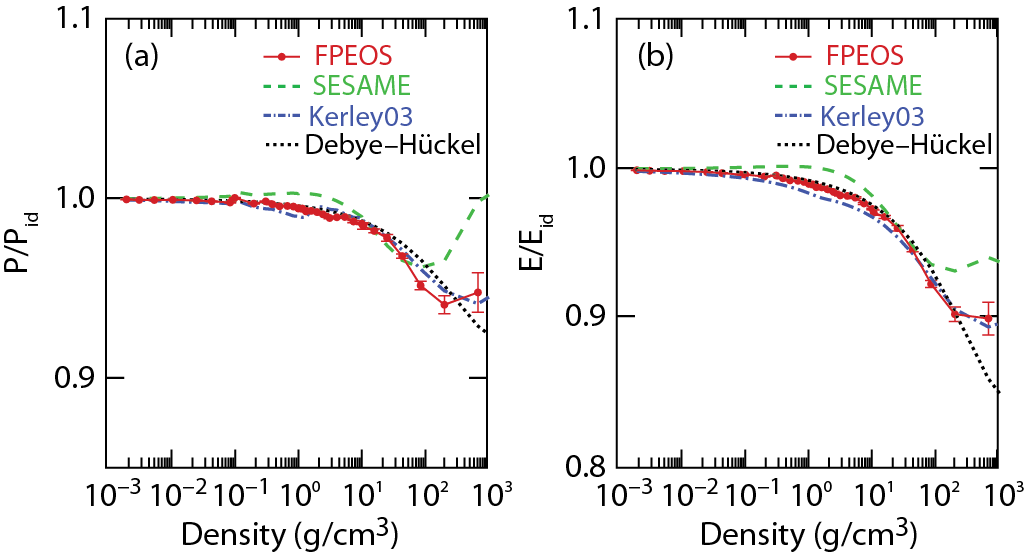
Figure 9: (Color online) Same as Fig. 7 but for a different temperature of $4\times 10^{6}$ K.

In Figs. 10$-$13, we compare the pressure and energy versus temperature for specific densities of 0.1, 1.0, 10.0, 84.19 g/cm³. At high temperature where the plasma is fully ionized, the Debye-Hückel model well reproduces the FPEOS pressures and energies very well. It is interesting to note that the SESAME table overestimates the pressure and energy even for a fully ionized plasma at densities greater than 1.0 g/cm³ as shown in Figs. 11$-$13. For a very low density of 0.1 g/cm³, Fig. 10 shows that the improved Kerley03 agrees very well with FPEOS, while the SESAME results are noticeably higher. Moreover, the improvements made to Kerley03 have resulted in remarkable agreement with FPEOS for intermediate densities of 0.1 and 10.0 g/cm³ depicted by Figs. 11 and 12. Only a small deviation in the internal energy between Kerley03 and our FPEOS results can be found at the lowest temperature for 1.0 g/cm³.

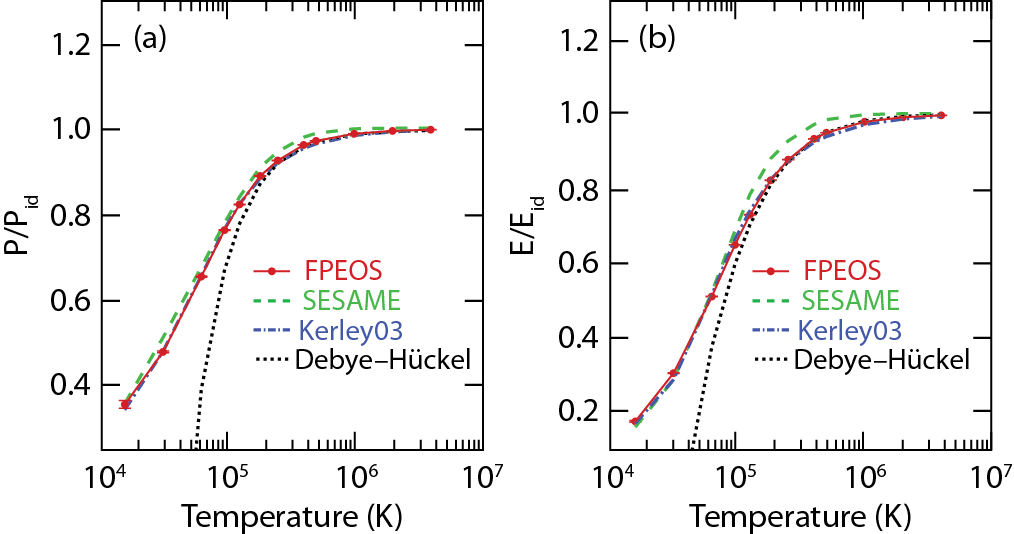
Figure 10: (Color online) Pressure (a) and energy (b) as a function of temperature from FPEOS, SESAME, and Kerley03 tables for deuterium density of 0.1 g/cm³.

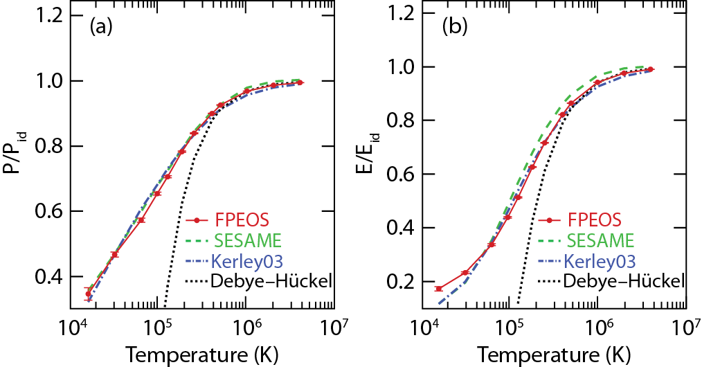
Figure 11: (Color online) Same as Fig. 10 but for a different deuterium density of 1.0 g/cm³.

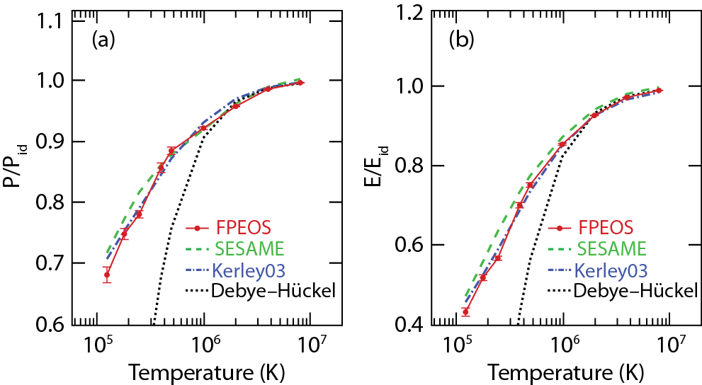
Figure 12: (Color online) Same as Fig. 10 but for a higher deuterium density of 10.0 g/cm³.

At a higher density of 84.19 g/cm³, the SESAME EOS again significantly deviates from both the FPEOS and the Kerley03 EOS as is illustrated by Fig. 13. The latter two EOS tables give very similar results in internal energy almost for the entire temperature range, though the pressures predicted by Kerley03 are higher than the FPEOS ones for temperatures varying from $2\times 10^{6}$ K to $2\times 10^{7}$ K. In contrast to the significant EOS differences seen from SESAME, the improved Kerley03 table is overall in better agreement with the FPEOS table, although subtle discrepancies and an artificial pressure cusp still exist in the Kerley03 EOS.

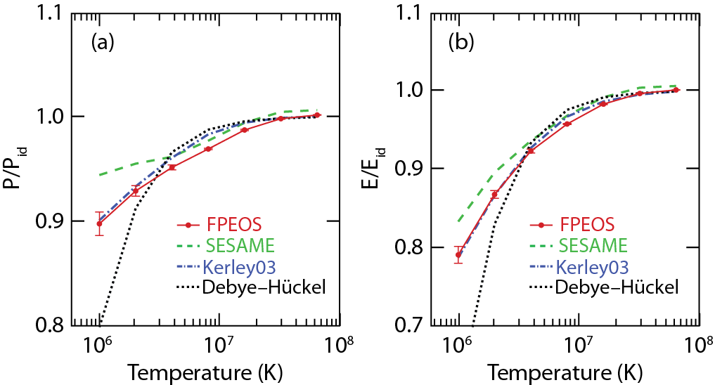
Figure 13: (Color online) Same as Fig. 10 but for much higher deuterium density 84.19 g/cm³.

VI Applications to ICF

With the EOS comparisons discussed above, we now investigate what differences can be observed when these EOS tables are applied to simulate ICF shock timing experiments and target implosions. Using radiation-hydrodynamics codes, both one-dimensional LILAC LILAC and two-dimensional DRACO draco , for simulations of experiments, we can explore the implications of our first-principles equation of state table for the understanding and design of ICF targets.

We first study the shock timing experiments shock-timing1 ; shock-timing2 performed on the Omega laser facility. As the fuel entropy in ICF implosions is set by a sequence of shocks, the timing of shock waves in liquid deuterium is extremely important for the ICF target performance. In shock timing experiments, the carbon deuterium (CD) spherical shell, 900 $\mu m$ in diameter and 10 $\mu m$ thick, in a cone-in-shell geometry shock-timing1 were filled with liquid deuterium. VISAR (velocity interferometery system for any reflector) was used to measure the shock velocity. As is shown in Fig. 14(a), the triple-picket laser pulses are designed to launch three shocks into the liquid deuterium. The experimental results are plotted in Fig. 14(b), in which the shock front velocity is shown as a function of time. One finds that when the second shock catches up the first one at around 1.5 ns, the shock-front velocity exhibits a sudden jump. Another velocity jump at $2.2$ ns occurs when the third strong shock overtakes the previous two. With the hydro-code LILAC, we have simulated the shock timing experiments using different EOS tables including FPEOS, SESAME, Kerley03, and QEOS qeos . The radiation hydro-simulations have used the standard flux-limited ($f=0.06$) thermal transport model, although a nonlocal model has resulted in better agreement with experiment for the speed of first shock shock-timing2 . The results of FPEOS, SESAME and Kerley03 are in good agreement with the experimental observation, while the QEOS predicts s much lower shock velocity and early catching up time. The shock timing experiments can only explore a small range of deuterium densities (0.6$-$2.5 g/cm³) and temperatures ($3-10$ eV). In these plasma conditions the SESAME and Kerley03 have been adjusted Kerley2003 to match to the first-principles calculations, which can be seen in Fig. 11. Thus, the shock velocity differences predicted by the FPEOS, SESAME, and Kerley03 are very small in such plasma conditions.

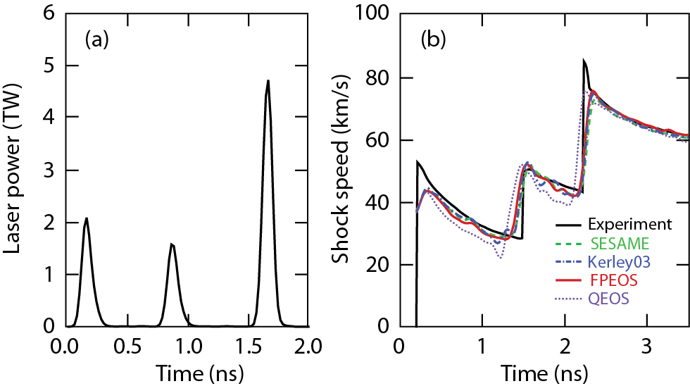
Figure 14: (Color online) (a) The triple-picket pulse shape for shock-timing experiments using cryogenic deuterium; and (b) the measured shock speed in liquid-D₂ (black solid-line) comparing with hydro-dynamics predictions using the SESAME, FPEOS, Kerley03, and QEOS models.

Next, we examine the implications of coupling and degeneracy effects in ICF implosions. The possible differences in target compression and fusion yields of ICF implosions are investigated through radiation hydro-simulations using FPEOS in comparison to results predicted by SESAME and Kerley03. The LILAC-simulation results are compared in Figs. 15 and 16, respectively, for a $DT$ implosion on OMEGA and a hydro-equivalent direct-drive design on the NIF. In Figs. 15(a) and 16(a), we plot the laser pulse shapes consisting of triple-pickets and the step-main-pulse. The cryogenic OMEGA DT target (860 $\mu m$ diameter) has a 10-$\mu m$ deuterated plastic ablator and $\sim 65~{}\mu m$ of DT ice. Figure  15(b) shows the density and temperature profiles at the end of the laser pulse ($t=3.8$ ns) from the FPEOS (red/solid line), the SESAME (green/dashed line), and the Kerley03 (blue/dot-dashed line) simulations. AT this time the shell has converged to a radius of $\sim 160~{}\mu m$ from its original radius of $\sim 430~{}\mu m$. The shell?s peak density and average temperature were $\rho\simeq 5.6$ g/cm³ and $T\simeq 21$ eV, which correspond to the coupled and degenerate regimes with $\Gamma\simeq 1.22$ and $\theta\simeq 0.47$. It is shown that the FPEOS simulation predicted $\sim 10$% lower peak density but $\sim 15$% higher temperature relative to the SESAME prediction. As is shown by the comparisons made in Fig.  8 and in Ref. [FPEOS_PRL ], the FPEOS predicts slightly stiffer deuterium than SESAME at the similar temperature regime. This explains the lower peak density seen in Fig. 15(b). The $\sim 15$% higher temperature in the FPEOS case was originated from the lower internal energy [see Fig.  8(b)]. Since the laser ablation does the same work/energy to the shell compression and its kinetic motion, a lower internal energy in FPEOS means more energy is partitioned to heat the shell, thereby resulting in a higher temperature. Such a temperature increase and density drop can have consequences in the implosion performance. Despite the subtle EOS differences discussed above, the Kerley03 simulation show very similar results when compared to FPEOS. Only small differences in temperature profile can be seen between the FPEOS and Kerley03 simulations, both of which are in remarkable contrast to the SESAME case. Figure  15(c) show the density profile at the peak compression, in which the predicted peak density ($\rho_{p}\simeq 210$ g/cm³) is $\sim 25$% lower according to FPEOS and Kerley03 compared to the SESAME prediction ($\rho_{p}\simeq 260$ g/cm³). The history of areal density $\rho R$-evolution and neutron production were shown in Fig. 15(d). One sees that the peak $\rho R$ and neutron yield are also reduced by $\sim 10$% - 20% when the FPEOS and Kerley03 are compared to the SESAME predictions. The absolute neutron yield drops from $\sim 8.44\times 10^{13}$ predicted by SESAME to $\sim 6.91\times 10^{13}$ (FPEOS) and $\sim 6.93\times 10^{13}$ (Kerley03).

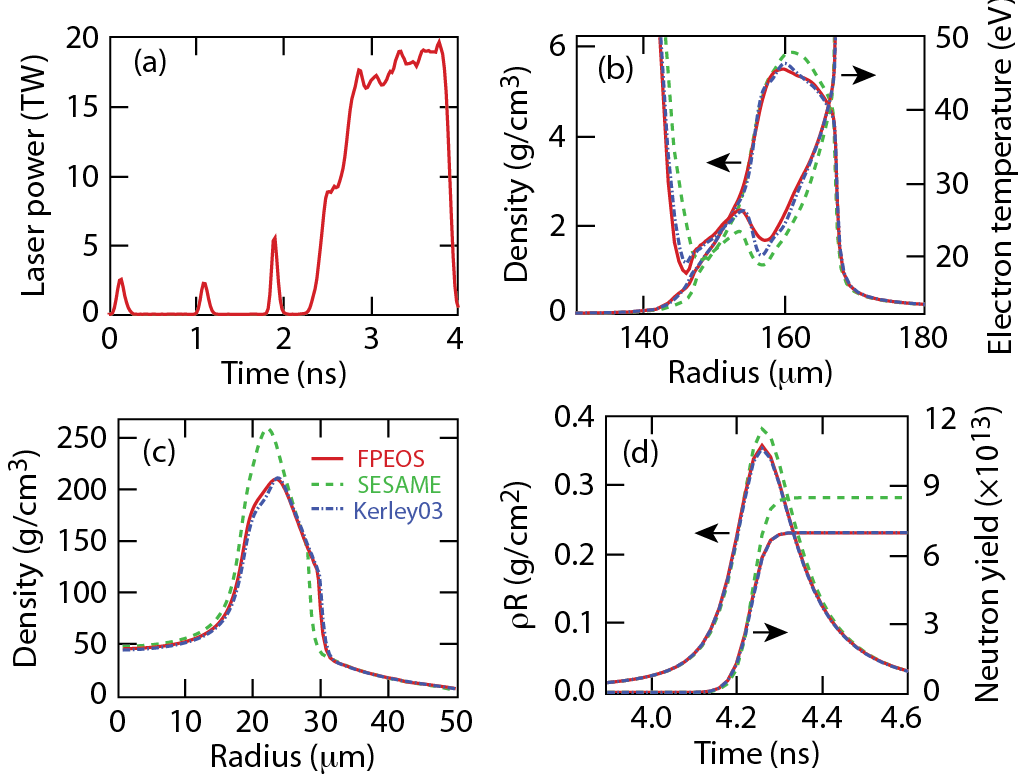
Figure 15: (Color online) The hydro-code simulations of a cryogenic DT implosion on OMEGA using the three different EOS tables including SESAME, FPEOS, and Kerley03: (a) The laser pulse shape; (b) The density-temperature profiles of the imploding DT shell at the middle of main laser pulse ($t=3.8$ ns); (c) the density profile at the peak compression (t=4.26 ns); and (d) the areal density $\rho R$ and yield as a function of time.

Figure  16 shows the similar effects for the hydro-equivalent direct-drive NIF design with 1-MJ laser energy. The NIF target ($\phi=2.954$-mm) consists of 27-$\mu m$ plastic ablator and 170-$\mu m$ DT ice. The triple-picket drive pulse has a total duration of $\sim 11.4$ ns and a peak power of $\sim 240$-TW. We also found a decrease in $\rho_{p}$ and a slight temperature increase for the FPEOS and Kerley03 relative to SESAME simulations near the end of the laser pulse ($t=9.2$ ns), shown by Fig.  16(b). The peak density at the stagnation dropped from 481 (SESAME) to $\sim 445$ g/cm³ (FPEOS/Kerley03), which is indicated by Fig. 16(c). The resulting $\rho R$ and neutron yield as a function of time is plotted in Fig. 16(d). The yield dropped from the SESAME value of $Y\simeq 1.75\times 10^{19}$ to $Y\simeq 1.57\times 10^{19}$ (FPEOS) and $Y\simeq 1.55\times 10^{19}$ (Kerley03). Consequently, the energy gain decreased from 49.1 (SESAME) to 44.2 (FPEOS) and 43.8 (Kerley03). It is noted that the $\sim 11$% gain reduction for this design is much modest than the $1.5$-MJ NIF design discussed in Ref. [FPEOS_PRL ] in which more than $\sim 20$% gain difference has been seen between FPEOS and SESAME simulations. This is attributed to the different density-temperature trajectories that the two designed implosions undergo, in which the EOS variations among FPEOS, SESAME and Kerley03 are different.

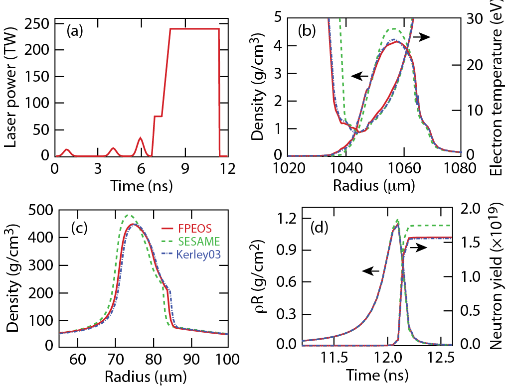
Figure 16: (Color online) Similar to Fig. 15 but for a hydro-equivalent direct drive, 1 MJ ignition design for NIF.

Finally, we discuss the implications of the coupling and degeneracy effects in FPEOS to ICF target performance beyond the 1D physics studied above. As we knew that various perturbations seeded by target roughness and lasers can grow via the Rayleigh-Taylor (RT) instability RTs during the shell acceleration/deceleration phases in ICF implosions, it is important to properly simulate the RT growth of fusion fuel for understanding target performance (compression and neutron yields) my_POP_2009 ; my_POP_2010 . Since the RT growth depends on the compressibility of materials, the accurate equation-of-state of deuterium is essential to ICF designs. As an example, we have used our two-dimensional radiative hydro-code DRACO to simulate the cryogenic DT implosion on OMEGA [discussed in Fig. 15]. The various perturbation sources, including the target offset, ice roughness, and laser irradiation non-uniformities measured from experiments, have been taken into account up to a maximum mode of $l=150$. We have compared the FPEOS and SESAME simulation results in Fig. 17 for $t=3.85$ ns near the end of acceleration, in which the density contours are plotted in the $ZR$-plane (azimuthal symmetry with respect to the Z-axis is assumed). Visible differences in the DT shell density can even be seen by eye from Figs. 17(a) and (b). The FPEOS simulation resulted in more “holes” and density modulations along the shell than the SESAME case.

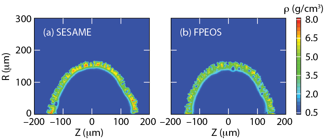
Figure 17: (Color online) The density contour plots at t=3.85 ns from two-dimensional DRACO simulations of the OMEGA cryogenic DT-implosion shown in Fig. 15, respectively using the SESAME (a) and the FPEOS (b) for the fuel DT. It is noted that the various perturbation sources have been included up to mode $\sl l=150$.

To further analyze the perturbation amplitudes, we have decomposed the ablation-surface modulations into a modal spectrum that is shown in Fig. 18(a), at the start of shell acceleration (t=3.0 ns). We find that the FPEOS predicted larger amplitudes than the SESAME case almost over the entire modal range. As the deuterium Hugoniot was shown in Ref. [FPEOS_PRL ], the FPEOS predicted softer deuterium compared to SESAME for pressures below $\sim 2$ Mbar. Thus, the softer deuterium can be more easily “imprinted” by the perturbations brought in via the series of shocks. This results in larger perturbation amplitudes in FPEOS than SESAME simulations. The Rayleigh-Taylor instability further amplifies these perturbations during the shell acceleration. As indicated by Fig. 18(b), the $\sigma_{rms}$ of fuel $\rho R$ modulation increases to a few mg/cm² at the end of the laser pulse. These perturbations penetrated into the inner surface of the DT-shell will become the seeds for further RT growth during the shell’s deceleration phase. They eventually distort the hot-spot temperature and density, thereby reducing the neutron production. At the end, we found that the SESAME simulation resulted in a neutron-averaged ion temperature of $\left<T_{i}\right>=2.6$ keV and a neutron yield of $Y=5.2\times 10^{12}$; while due to the larger perturbations predicted the FPEOS simulation has given an $\left<T_{i}\right>=2.3$ keV and neutron yield of $Y=3.7\times 10^{12}$, which is more close to experimental observations of $\left<T_{i}\right>=1.8\pm 0.5$ keV and $Y=1.9\times 10^{12}$.

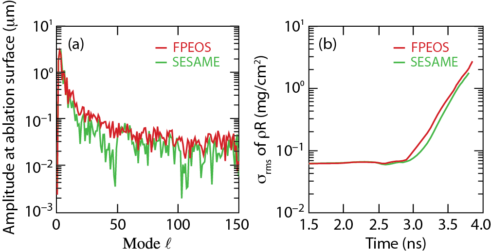
Figure 18: (Color online) (a) The modal spectrum of perturbation amplitude at the ablation surface for $t\simeq 3.0$ ns (the beginning of acceleration); (b) The perturbation growth in $\rho R$ as a function of time, analyzed from the 2D-DRACO simulations shown in Fig. 17.

VII Summary

In conclusion, we have derived a first-principles equation of state table of deuterium for ICF applications from PIMC calculations. The derived FPEOS table covers the whole plasma density and temperature conditions in low-adiabat ICF implosions. In comparison with the chemical model based SESAME table, the FPEOS table show significant difference in internal energy and pressure for coupled and degenerate plasma conditions; while the recently improved Kerley03 table exhibited fewer and smaller discrepancies when compared to the FPEOS predictions temperature higher than $\sim 10$-eV. Although subtle differences at lower temperatures ($T<10$ eV) and moderate densities ($1-10$ g/cm³) have been identified and an artificial pressure cusp still exists in the Kerley03 table, radiation hydro-simulations of cryogenic ICF implosions using the FPEOS and Kerley03 tables have given similar peak density, areal density $\rho R$, and neutron yield, which are remarkably different from the SESAME simulations. Both the FPEOS and the Kerley03 predicted $\sim 25$% less peak density, $\sim 10$% smaller $\rho R$, and $\sim 10$%-20% less neutron yield, when compared to the SESAME case. Two-dimensional simulations further demonstrated the significant differences in target performance between the FPEOS and SESAME simulations. In general, the FPEOS simulations resulted in better agreement with experimental observations in terms of ion temperature and neutron yield. It is also noted that the extreme conditions covered by the FPEOS table are also important in astrophysics and planetary sciences, for example, to model the evolution of stars star and to understand the thermodynamical properties of stellar matter astro .

*E-mail: shu@lle.rochester.edu

References

- (1) J. Nuckolls, L. Wood, A. Thiessen, and G. Zimmerman, Nature (London) 239, 139 (1972); S. Atzeni and J. Meyer-ter-Vehn, The Physics of Inertial Fusion (Clarendon Press, Oxford, 2004).
- (2) R. L. McCrory et al., Phys. Plasmas 15, 055503 (2008); D.D. Meyerhofer et al., Nuclear Fusion 51, 053010 (2011).
- (3) J. D. Lindl, Phys. Plasmas 2, 3933 (1995).
- (4) R. Betti and C. Zhou, Phys. Plasmas 12, 110702 (2005); R. Betti et al., Plasma Phys. Controlled Fusion 48, B153 (2006).
- (5) V. N. Goncharov, T. C. Sangster, T. R. Boehly, S. X. Hu, I. V. Igumenshchev, F. J. Marshall, R. L. McCrory, D. D. Meyerhofer, P. B. Radha, W. Seka, S. Skupsky, C. Stoeckl, D. T. Casey, J. A. Frenje, and R. D. Petrasso, Phys. Rev. Lett. 104, 165001 (2010).
- (6) E. M. Campbell and W. J. Hogan, Plasma Phys. Control. Fusion 41, B39 (1999).
- (7) T. R. Boehly et al., Opt. Commun. 133, 495 (1997).
- (8) S. X. Hu et al., Phys. Rev. Lett. 100, 185003 (2008).
- (9) G. I. Kerley, Phys. Earth Planet. Inter. 6, 78 (1972).
- (10) G. I. Kerley, Sandia National Laboratory, Technical Report No. SAND2003-3613, 2003 (unpublished).
- (11) D. Saumon, G. Chabrier, Phys. Rev. A46, 2084 (1992).
- (12) M. Ross, Phys. Rev. B58, 669 (1998).
- (13) F. J. Rogers, Contrib. Plasma Phys. 41, 179 (2001).
- (14) H. Juranek, R. Redmer, Y. Rosenfeld, J. Chem. Phys. 117, 1768 (2002).
- (15) C. Pierleoni et al., Phys. Rev. Lett. 73, 2145 (1994).
- (16) W. R. Magro et al., Phys. Rev. Lett. 76, 1240 (1996).
- (17) B. Militzer, D.M. Ceperley, Phys. Rev. Lett. 85, 1890 (2000).
- (18) B. Militzer, D. M. Ceperley , J. D. Kress, J. D. Johnson, L. A. Collins, and S. Mazevet, Phys. Rev. Lett. 87, 275502 (2001).
- (19) J. Delettrez et al., Phys. Rev. A 36, 3926 (1987).
- (20) S. X. Hu, B. Militzer, V. N. Goncharov, and S. Skupsky, Phys. Rev. Lett. 104, 235003 (2010).
- (21) M. S. Murillo and M. W. C. Dharma-wardana, Phys. Rev. Lett. 100, 205005 (2008); B. Jeon et al., Phys. Rev. E78, 036403 (2008); G. Dimonte and J. Daligault, Phys. Rev. Lett. 101, 135001 (2008); J. N. Glosli et al., Phys. Rev. E78, 025401(R) (2008); L. X. Benedict et al., Phys. Rev. Lett. 102, 205004 (2009); B. Xu and S. X. Hu, Phys. Rev. E 84, 016408 (2011).
- (22) V. Recoules, F. Lambert, A. Decoster, B. Canaud, and J. Clerouin et al., Phys. Rev. Lett. 102, 075002 (2009).
- (23) E. L. Pollock, B. Militzer, Phys. Rev. Lett. 92, 021101 (2004).
- (24) J. D. Kress, J. S. Cohen, D. A. Horner, F. Lambert, and L. A. Collins, Phys. Rev. E 82, 036404 (2010).
- (25) L. B. Da Silva et al., Phys. Rev. Lett. 78, 483 (1997).
- (26) G. W. Collins et al., Science 281, 1178 (1998).
- (27) G. W. Collins et al., Phys. Plasmas 5, 1864 (1998).
- (28) A. N. Mostovych et al., Phys. Rev. Lett. 85, 3870 (2000); Phys. Plasmas 8, 2281 (2001).
- (29) T. R. Boehly et al., Phys. Plasmas 11, L49 (2004).
- (30) D. G. Hicks et al., Phys. Rev. B79, 014112 (2009).
- (31) M. D. Knudson et al., Phys. Rev. Lett. 87, 225501 (2001); ibid 90, 035505 (2003).
- (32) M. D. Knudson et al., Phys. Rev. B69, 144209 (2004).
- (33) S. I. Belov et al., JETP Lett. 76, 433 (2002).
- (34) V. E. Fortov et al., Phys. Rev. Lett. 99, 185001 (2007).
- (35) L. A. Collins et al., Phys. Rev. E52, 6202 (1995).
- (36) T. J. Lenosky et al., Phys. Rev. B61, 1 (2000).
- (37) G. Galli et al., Phys. Rev. B61, 909 (2000).
- (38) L. A. Collins et al., Phys. Rev. B63, 184110 (2001).
- (39) J. Clerouin, J.F. Dufreche, Phys. Rev. E64, 066406 (2001).
- (40) M. P. Desjarlais, Phys. Rev. B68, 064204 (2003).
- (41) S. A. Bonev, B. Militzer, G. Galli, Phys. Rev. B69, 014101 (2004).
- (42) L. A. Collins (private communication).
- (43) F. Lambert, J. Clerouin, and G. Zerah, Phys. Rev. E 73, 016403 (2006); F. Lambert, J. Clerouin, and S. Mazevet, Europhys. Lett. 75, 681 (2006); D. A. Horner, F. Lambert, J. D. Kress, and L. A. Collins, Phys. Rev. B 80, 024305 (2009).
- (44) B. Militzer, Phys. Rev. Lett. 97, 175501 (2006).
- (45) B. Militzer, Phys. Rev. B 79, 155105 (2009).
- (46) B. Militzer, PhD Thesis (University of Illinois, 2000).
- (47) D. M. Ceperley, Rev. Mod. Phys. 67, 279 (1995).
- (48) D. M. Ceperley, J. Stat. Phys. 63, 1237 (1991).
- (49) D. M. Ceperley, in Monte Carlo and Molecular Dynamics of Condensed Matter Systems, edited by K. Binder and G. Ciccotti (Editrice Compositori, Bologna, Italy, 1996).
- (50) B. Militzer and E. L. Pollock, Phys. Rev. E61, 3470 (2000).
- (51) B. Militzer, W. Magro, D. M. Ceperley, Contrib. Plasma Phys. 39, 151 (1999).
- (52) P. Debye and E. Hückel, Phys. Z. 24, 185 (1923).
- (53) D. Keller, T. J. B. Collins, J. A. Delettrez, P. W. McKenty, P. B. Radha, B. Whitney, and G. A. Moses, Bull. Am. Phys. Soc. 44, 37 (1999); P. B. Radha, T. J. B. Collins, J. A. Delettrez, Y. Elbaz, R. Epstein, V. Yu. Glebov, V. N. Goncharov, R. L. Keck, J. P. Knauer, J. A. Marozas, F. J. Marshall, R. L. McCrory, P. W. McKenty, D. D. Meyerhofer, S. P. Regan, T. C. Sangster, W. Seka, D. Shvarts, S. Skupsky, Y. Srebro, and C. Stoeckl, Phys. Plasmas 12, 056307 (2005); S. X. Hu, V. A. Smalyuk, V. N. Goncharov, S. Skupsky, T. C. Sangster, D. D. Meyerhofer, and D. Shvarts, Phys. Rev. Lett. 101, 055002 (2008).
- (54) T. R. Boehly et al., Phys. Plasmas 16, 056302 (2009).
- (55) T. R. Boehly, V. N. Goncharov, W. Seka, M. A. Barrios, P. M. Celliers, D. G. Hicks, G. W. Collins, S. X. Hu, J. A. Marozas, and D. D. Meyerhofer, Phys. Rev. Lett. 106, 195005 (2011).
- (56) R. More, K. H. Warren, D. A. Young, and G. Zimmermann, Phys. Fluids 31, 3059 (1988).
- (57) B. A. Remington, S. V. Weber, M. M. Marinak, S. W. Haan, J. D. Kilkenny, R. Wallace, and G. Dimonte, Phys. Rev. Lett. 73, 545 (1994); H. Azechi, T. Sakaiya, S. Fujioka, Y. Tamari, K. Otani, K. Shigemori, M. Nakai, H. Shiraga, N. Miyanaga, and K. Mima, ibid. 98, 045002 (2007); V. A. Smalyuk, S. X. Hu, V. N. Goncharov, D. D. Meyerhofer, T. C. Sangster, D. Shvarts, C. Stoeckl, B. Yaakobi, J. A. Frenje, and R. D. Petrasso, ibid. 101, 025002 (2008); V. A. Smalyuk, S. X. Hu, V. N. Goncharov, D. D. Meyerhofer, T. C. Sangster, C. Stoeckl, and B. Yaakobi, Phys. Plasmas 15, 082703 (2008); V. A. Smalyuk, S. X. Hu, J. D. Hager, J. A. Delettrez, D. D. Meyerhofer, T. C. Sangster, and D. Shvarts, Phys. Rev. Lett. 103, 105001 (2009); V. A. Smalyuk, S. X. Hu, J. D. Hager, J. A. Delettrez, D. D. Meyerhofer, T. C. Sangster, and D. Shvarts, Phys. Plasmas 16, 112701 (2009).
- (58) S. X. Hu et al., Phys. Plasmas 16, 112706 (2009).
- (59) S. X. Hu et al., Phys. Plasmas 17, 102706 (2010).
- (60) F. J. Rogers and A. Nayfonov, Astrophys. J. 576, 1064 (2002).
- (61) W. Stolzmann and T. Blöcker, Astron. Astrophys. 361, 1152 (2000).