Solving Factored MDPs with Hybrid State and Action Variables

Abstract

Efficient representations and solutions for large decision problems with continuous and discrete variables are among the most important challenges faced by the designers of automated decision support systems. In this paper, we describe a novel hybrid factored Markov decision process (MDP) model that allows for a compact representation of these problems, and a new hybrid approximate linear programming (HALP) framework that permits their efficient solutions. The central idea of HALP is to approximate the optimal value function by a linear combination of basis functions and optimize its weights by linear programming. We analyze both theoretical and computational aspects of this approach, and demonstrate its scale-up potential on several hybrid optimization problems.

1 Introduction

A dynamic decision problem with components of uncertainty can be very often formulated as a Markov decision process (MDP). An MDP represents a controlled stochastic process whose dynamics is described by state transitions. Objectives of the control are modeled by rewards (or costs), which are assigned to state-action configurations. In the simplest form, the states and actions of an MDP are discrete and unstructured. These models can be solved efficiently by standard dynamic programming methods (?, ?, ?).

Unfortunately, textbook models rarely meet the practice and its needs. First, real-world decision problems are naturally described in a factored form and may involve a combination of discrete and continuous variables. Second, there are no guarantees that compact forms of the optimal value function or policy for these problems exist. Therefore, hybrid optimization problems are usually discretized and solved approximately by the methods for discrete-state MDPs. The contribution of this work is a principled, sound, and efficient approach to solving large-scale factored MDPs that avoids this discretization step.

Our framework is based on approximate linear programming (ALP) (?), which has been already applied to solve decision problems with discrete state and action variables efficiently (?, ?, ?). These applications include context-specific planning (?), multiagent planning (?), relational MDPs (?), and first-order MDPs (?). In this work, we show how to adapt ALP to solving large-scale factored MDPs in hybrid state and action spaces.

The presented approach combines factored MDP representations (Sections 3 and 4) and optimization techniques for solving large-scale structured linear programs (Section 6). This leads to various benefits. First, the quality and complexity of value function approximations is controlled by using basis functions (Section 3.2). Therefore, we can prevent an exponential blowup in the complexity of computations when other techniques cannot. Second, we always guarantee that HALP returns a solution. Its quality naturally depends on the choice of basis functions. As analyzed in Section 5.1, if these are selected appropriately, we achieve a close approximation to the optimal value function $V^{\ast}$. Third, a well-chosen class of basis functions yields closed-form solutions to the backprojections of our value functions (Section 5.2). This step is important for solving hybrid optimization problems more efficiently. Finally, solving hybrid factored MDPs reduces to building and satisfying relaxed formulations of the original problem (Section 6). The formulations can be solved efficiently by the cutting plane method, which has been studied extensively in applied mathematics and operations research.

For better readability of the paper, our proofs are deferred to Appendix A. The following notation is adopted throughout the work. Sets and their members are represented by capital and small italic letters as $\mathcal{S}$ and $s$, respectively. Sets of variables, their subsets, and members of these sets are denoted by capital letters as ${\bf X}$, ${\bf X}_{i}$, and $X_{i}$. In general, corresponding small letters represent value assignments to these objects. The subscripted indices $D$ and $C$ denote the discrete and continuous variables in a variable set and its value assignment. The function $\mathrm{Dom}(\cdot)$ computes the domain of a variable or the domain of a function. The function $\mathsf{Par}(\cdot)$ returns the parent set of a variable in a graphical model (?, ?).

2 Markov Decision Processes

Markov decision processes (?) provide an elegant mathematical framework for modeling and solving sequential decision problems in the presence of uncertainty. Formally, a finite-state Markov decision process (MDP) is given by a 4-tuple $\mathcal{M}=(\mathcal{S},\mathcal{A},P,R)$, where $\mathcal{S}=\left\{s_{1},\dots,s_{n}\right\}$ is a set of states, $\mathcal{A}=\left\{a_{1},\dots,a_{m}\right\}$ is a set of actions, $P:\mathcal{S}\times\mathcal{A}\times\mathcal{S}\rightarrow[0,1]$ is a stochastic transition function of state dynamics conditioned on the preceding state and action, and $R:\mathcal{S}\times\mathcal{A}\rightarrow\mathbb{R}$ is a reward function assigning immediate payoffs to state-action configurations. Without loss of generality, the reward function is assumed to be nonnegative and bounded from above by a constant $R_{\mathrm{max}}$ (?). Moreover, we assume that the transition and reward models are stationary and known a priori.

Once a decision problem is formulated as an MDP, the goal is to find a policy $\pi:\mathcal{S}\rightarrow\mathcal{A}$ that maximizes some objective function. In this paper, the quality of a policy $\pi$ is measured by the infinite horizon discounted reward:

$$\mathrm{E}_{\pi}\!\left[\left.\sum_{t=0}^{\infty}\gamma^{t}R(s^{(t)},\pi(s^{(t)}))\right|s^{(0)}\sim\varphi\right],$$ (1)

where $\gamma\in[0,1)$ is a discount factor, $s^{(t)}$ is the state at the time step $t$, and the expectation is taken with respect to all state-action trajectories that start in the states $s^{(0)}$ and follow the policy $\pi$ thereafter. The states $s^{(0)}$ are chosen according to a distribution $\varphi$. This optimality criterion assures that there exists an optimal policy $\pi^{\ast}$ which is stationary and deterministic (?). The policy is greedy with respect to the optimal value function $V^{\ast}$, which is a fixed point of the Bellman equation (?):

$$V^{\ast}(s)=\max_{a}\left[R(s,a)+\gamma\sum_{s^{\prime}}P(s^{\prime}\mid s,a)V^{\ast}(s^{\prime})\right].$$ (2)

The Bellman equation plays a fundamental role in all dynamic programming (DP) methods for solving MDPs (?, ?), including value iteration, policy iteration, and linear programming. The focus of this paper is on linear programming methods and their refinements. Briefly, it is well known that the optimal value function $V^{\ast}$ is a solution to the linear programming (LP) formulation (?):

minimize $$\quad\sum_{s}\psi(s)V(s)$$ (3)

subject to: $$\quad V(s)\geq R(s,a)+\gamma\sum_{s^{\prime}}P(s^{\prime}\mid s,a)V(s^{\prime})\quad\forall\ s\in\mathcal{S},a\in\mathcal{A};$$

where $V(s)$ represents the variables in the LP, one for each state $s$, and $\psi(s)>0$ is a strictly positive weighting on the state space $\mathcal{S}$. The number of constraints equals to the cardinality of the cross product of the state and action spaces $\left|\mathcal{S}\times\mathcal{A}\right|$.

Linear programming and its efficient solutions have been studied extensively in applied mathematics and operations research (?). The simplex algorithm is a common way of solving LPs. Its worst-case time complexity is exponential in the number of variables. The ellipsoid method (?) offers polynomial time guarantees but it is impractical for solving LPs of even moderate size.

The LP formulation (3) can be solved compactly by the cutting plane method (?) if its objective function and constraint space are structured. Briefly, this method searches for violated constraints in relaxed formulations of the original LP. In every step, we start with a relaxed solution $V^{(t)}$, find a violated constraint given $V^{(t)}$, add it to the LP, and resolve for a new vector $V^{(t+1)}$. The method is iterated until no violated constraint is found, so that $V^{(t)}$ is an optimal solution to the LP. The approach has a potential to solve large structured linear programs if we can identify violated constraints efficiently (?). The violated constraint and the method that found it are often referred to as a separating hyperplane and a separation oracle, respectively.

Delayed column generation is based on a similar idea as the cutting plane method, which is applied to the column space of variables instead of the row space of constraints. Bender’s and Dantzig-Wolfe decompositions reflect the structure in the constraint space and are often used for solving large structured linear programs.

3 Discrete-State Factored MDPs

Many real-world decision problems are naturally described in a factored form. Discrete-state factored MDPs (?) allow for a compact representation of this structure.

3.1 Factored Transition and Reward Models

A discrete-state factored MDP (?) is a 4-tuple $\mathcal{M}=({\bf X},\mathcal{A},P,R)$, where ${\bf X}=\left\{X_{1},\dots,X_{n}\right\}$ is a state space described by a set of state variables, $\mathcal{A}=\left\{a_{1},\dots,a_{m}\right\}$ is a set of actions, $P({\bf X}^{\prime}\mid{\bf X},\mathcal{A})$ is a stochastic transition model of state dynamics conditioned on the preceding state and action, and $R$ is a reward function assigning immediate payoffs to state-action configurations. The state of the system is completely observed and represented by a vector of value assignments ${\bf x}=(x_{1},\dots,x_{n})$. We assume that the values of every state variable $X_{i}$ are restricted to a finite domain $\mathrm{Dom}(X_{i})$.

Transition model: The transition model is given by the conditional probability distribution $P({\bf X}^{\prime}\mid{\bf X},\mathcal{A})$, where ${\bf X}$ and ${\bf X}^{\prime}$ denote the state variables at two successive time steps. Since the complete tabular representation of $P({\bf X}^{\prime}\mid{\bf X},\mathcal{A})$ is infeasible, we assume that the transition model factors along ${\bf X}^{\prime}$ as:

$$P({\bf X}^{\prime}\mid{\bf X},a)=\prod_{i=1}^{n}P(X_{i}^{\prime}\mid\mathsf{Par}(X_{i}^{\prime}),a)$$ (4)

and can be described compactly by a dynamic Bayesian network (DBN) (?). This DBN representation captures independencies among the state variables ${\bf X}$ and ${\bf X}^{\prime}$ given an action $a$. One-step dynamics of every state variable is modeled by its conditional probability distribution $P(X_{i}^{\prime}\mid\!\mathsf{Par}(X_{i}^{\prime}),a)$, where $\mathsf{Par}(X_{i}^{\prime})\!\subseteq{\bf X}$ denotes the parent set of $X_{i}^{\prime}$. Typically, the parent set is a subset of state variables which simplifies the parameterization of the model. In principle, the parent set can be extended to the state variables ${\bf X}^{\prime}$. Such an extension poses only few new challenges when solving the new problems efficiently (?). Therefore, we omit the discussion on the modeling of intra-layer dependencies in this paper.

Reward model: The reward model factors similarly to the transition model. In particular, the reward function $R({\bf x},a)=\sum_{j}R_{j}({\bf x}_{j},a)$ is an additive function of local reward functions defined on the subsets ${\bf X}_{j}$ and $\mathcal{A}$. In graphical models, the local functions can be described compactly by reward nodes $R_{j}$, which are conditioned on their parent sets $\mathsf{Par}(R_{j})={\bf X}_{j}\cup\mathcal{A}$. To allow this representation, we formally extend our DBN to an influence diagram (?).

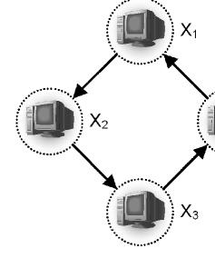
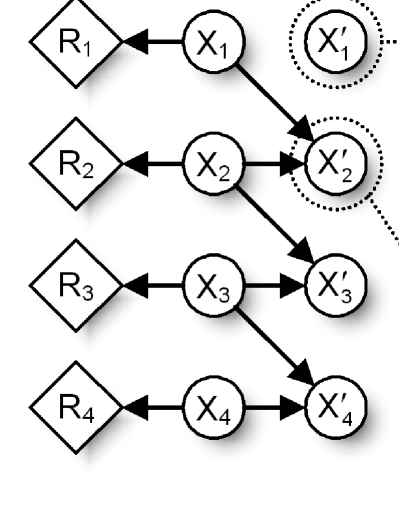
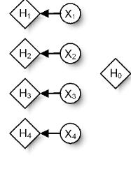
(a)	(b)	(c)

Figure 1: a. Four computers in a ring topology. Direction of propagating failures is denoted by arrows. b. A graphical representation of factored transition and reward models after taking an action $a_{1}$ in the 4-ring topology. The future state of the server $X_{1}^{\prime}$ is independent of the rest of the network because the server is rebooted. Reward nodes $R_{1}$ and $R_{j}$ ($j\geq 2$) denote the components $2x_{1}$ and $x_{j}$ ($j\geq 2$) of the reward model. c. A graphical representation of the linear value function approximation $V^{\bf w}({\bf x})=w_{0}+\sum_{i=1}^{4}w_{i}x_{i}$ in the 4-ring topology. Reward nodes $H_{0}$ and $H_{i}$ ($i\geq 1$) denote the value function components $w_{0}$ and $w_{i}x_{i}$ ($i\geq 1$).

Example 1 (?)

To illustrate the concept of a factored MDP, we consider a network administration problem, in which the computers are unreliable and fail. The failures of these computers propagate through network connections to the whole network. For instance, if the server $X_{1}$ (Figure 1a) is down, the chance that the neighboring computer $X_{2}$ crashes increases. The administrator can prevent the propagation of the failures by rebooting computers that have already crashed.

This network administration problem can be formulated as a factored MDP. The state of the network is completely observable and represented by $n$ binary variables ${\bf X}=\left\{X_{1},\dots,X_{n}\right\}$, where the variable $X_{i}$ denotes the state of the $i$-th computer: 0 (being down) or 1 (running). At each time step, the administrator selects an action from the set $\mathcal{A}=\left\{a_{1},\dots,a_{n+1}\right\}$. The action $a_{i}$ ($i\leq n$) corresponds to rebooting the $i$-th computer. The last action $a_{n+1}$ is dummy. The transition function reflects the propagation of failures in the network and can be encoded locally by conditioning on the parent set of every computer. A natural metric for evaluating the performance of an administrator is the total number of running computers. This metric factors along the computer states $x_{i}$ and can be represented compactly by an additive reward function:

$$R({\bf x},a)=2x_{1}+\sum_{j=2}^{n}x_{j}.$$

The weighting of states establishes our preferences for maintaining the server $X_{1}$ and workstations $X_{2},\dots,X_{n}$. An example of transition and reward models after taking an action $a_{1}$ in the 4-ring topology (Figure 1a) is given in Figure 1b.

3.2 Solving Discrete-State Factored MDPs

Markov decision processes can be solved by exact DP methods in polynomial time in the size of the state space ${\bf X}$ (?). Unfortunately, factored state spaces are exponential in the number of state variables. Therefore, the DP methods are unsuitable for solving large factored MDPs. Since a factored representation of an MDP (Section 3.1) may not guarantee a structure in the optimal value function or policy (?), we resort to value function approximations to alleviate this concern.

Value function approximations have been successfully applied to a variety of real-world domains, including backgammon (?, ?, ?), elevator dispatching (?), and job-shop scheduling (?, ?). These partial successes suggest that the approximate dynamic programming is a powerful tool for solving large optimization problems.

In this work, we focus on linear value function approximation (?, ?):

$$V^{\bf w}({\bf x})=\sum_{i}w_{i}f_{i}({\bf x}).$$ (5)

The approximation restricts the form of the value function $V^{\bf w}$ to the linear combination of $\left|{\bf w}\right|$ basis functions $f_{i}({\bf x})$, where ${\bf w}$ is a vector of optimized weights. Every basis function can be defined over the complete state space ${\bf X}$, but usually is limited to a small subset of state variables ${\bf X}_{i}$ (?, ?). The role of basis functions is similar to features in machine learning. They are often provided by domain experts, although there is a growing amount of work on learning basis functions automatically (?, ?, ?, ?, ?).

Example 2

To demonstrate the concept of the linear value function model, we consider the network administration problem (Example 1) and assume a low chance of a single computer failing. Then the value function in Figure 1c is sufficient to derive a close-to-optimal policy on the 4-ring topology (Figure 1a) because the indicator functions $f_{i}({\bf x})=x_{i}$ capture changes in the states of individual computers. For instance, if the computer $X_{i}$ fails, the linear policy:

$$u({\bf x})=\arg\max_{a}\left[R({\bf x},a)+\gamma\sum_{{\bf x}^{\prime}}P({\bf x}^{\prime}\mid{\bf x},a)V^{\bf w}({\bf x}^{\prime})\right]$$

immediately leads to rebooting it. If the failure has already propagated to the computer $X_{i+1}$, the policy recovers it in the next step. This procedure is repeated until the spread of the initial failure is stopped.

3.3 Approximate Linear Programming

Various methods for fitting of the linear value function approximation have been proposed and analyzed (?). We focus on approximate linear programming (ALP) (?), which recasts this problem as a linear program:

$$\textrm{minimize}_{\bf w} \quad\sum_{\bf x}\psi({\bf x})\sum_{i}w_{i}f_{i}({\bf x})$$ (6)

subject to: $$\quad\sum_{i}w_{i}f_{i}({\bf x})\geq R({\bf x},a)+\gamma\sum_{{\bf x}^{\prime}}P({\bf x}^{\prime}\mid{\bf x},a)\sum_{i}w_{i}f_{i}({\bf x}^{\prime})\quad\forall\ {\bf x}\in{\bf X},a\in\mathcal{A};$$

where ${\bf w}$ represents the variables in the LP, $\psi({\bf x})\geq 0$ are state relevance weights weighting the quality of the approximation, and $\gamma\sum_{{\bf x}^{\prime}}P({\bf x}^{\prime}\mid{\bf x},a)\sum_{i}w_{i}f_{i}({\bf x}^{\prime})$ is a discounted backprojection of the value function $V^{\bf w}$ (Equation 5). The ALP formulation can be easily derived from the standard LP formulation (3) by substituting $V^{\bf w}({\bf x})$ for $V({\bf x})$. The formulation is feasible if the set of basis functions contains a constant function $f_{0}({\bf x})\equiv 1$. We assume that such a basis function is always present. Note that the state relevance weights are no longer enforced to be strictly positive (Section 1). Comparing to the standard LP formulation (3), which is solved by the optimal value function $V^{\ast}$ for arbitrary weights $\psi(s)>0$, a solution $\widetilde{{\bf w}}$ to the ALP formulation depends on the weights $\psi({\bf x})$. Intuitively, the higher the weights, the higher the quality of the approximation $V^{\widetilde{{\bf w}}}$ in a corresponding state.

Since our basis functions are usually restricted to subsets of state variables (Section 3.2), summation terms in the ALP formulation can be computed efficiently (?, ?). For example, the order of summation in the backprojection term can be rearranged as $\gamma\sum_{i}w_{i}\sum_{{\bf x}_{i}^{\prime}}P({\bf x}_{i}^{\prime}\mid{\bf x},a)f_{i}({\bf x}_{i}^{\prime})$, which allows its aggregation in the space of ${\bf X}_{i}$ instead of ${\bf X}$. Similarly, a factored form of $\psi({\bf x})$ yields an efficiently computable objective function (?).

The number of constraints in the ALP formulation is exponential in the number of state variables. Fortunately, the constraints are structured. This results from combining factored transition and reward models (Section 3.1) with the linear approximation (Equation 5). As a consequence, the constraints can be satisfied without enumerating them exhaustively.

Example 3

The notion of a factored constraint space is important for compact satisfaction of exponentially many constraints. To illustrate this concept, let us consider the linear value function (Example 2) on the 4-ring network administration problem (Example 1). Intuitively, by combining the graphical representations of $P({\bf x}^{\prime}\mid{\bf x},a_{1})$, $R({\bf x},a_{1})$ (Figure 1b), and $V^{\bf w}({\bf x})$ (Figure 1c), we obtain a factored model of constraint violations:

$$\tau^{\bf w}({\bf x},a_{1})\ = \ \ V^{\bf w}({\bf x})-\gamma\sum_{{\bf x}^{\prime}}P({\bf x}^{\prime}\mid{\bf x},a_{1})V^{\bf w}({\bf x}^{\prime})-R({\bf x},a_{1})$$

$$\ = \ \ \sum_{i}w_{i}f_{i}({\bf x})-\gamma\sum_{i}w_{i}\sum_{{\bf x}_{i}^{\prime}}P({\bf x}_{i}^{\prime}\mid{\bf x},a_{1})f_{i}({\bf x}_{i}^{\prime})-R({\bf x},a_{1})$$

$$\ = \ \ w_{0}+\sum_{i=1}^{4}w_{i}x_{i}-\gamma w_{0}-\gamma w_{1}P(x_{1}^{\prime}=1\mid a_{1})-$$

$$\ \ \gamma\sum_{i=2}^{4}w_{i}P(x_{i}^{\prime}=1\mid x_{i},x_{i-1},a_{1})-2x_{1}-\sum_{j=2}^{4}x_{j}.$$

for an arbitrary solution ${\bf w}$ (Figure 2a). Note that this cost function:

$$\tau^{\bf w}({\bf x},a_{1})=\phi^{\bf w}+\sum_{i=1}^{4}\phi^{\bf w}(x_{i})+\sum_{i=2}^{4}\phi^{\bf w}(x_{i},x_{i-1})$$

is a linear combination of a constant $\phi^{\bf w}$ in ${\bf x}$, and univariate and bivariate functions $\phi^{\bf w}(x_{i})$ and $\phi^{\bf w}(x_{i},x_{i-1})$. It can be represented compactly by a cost network (?), which is an undirected graph over a set of variables ${\bf X}$. Two nodes in the graph are connected if any of the cost terms depends on both variables. Therefore, the cost network corresponding to the function $\tau^{\bf w}({\bf x},a_{1})$ must contain edges $X_{1}\!-\!X_{2}$, $X_{2}\!-\!X_{3}$, and $X_{3}\!-\!X_{4}$ (Figure 2b).

Savings achieved by the compact representation of constraints are related to the efficiency of computing $\arg\min_{{\bf x}}\tau^{\bf w}({\bf x},a_{1})$ (?). This computation can be done by variable elimination and its complexity increases exponentially in the width of the tree decomposition of the cost network. The smallest width of all tree decompositions is referred to as treewidth.

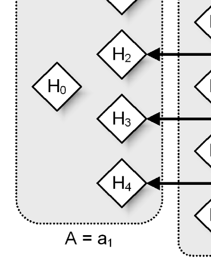
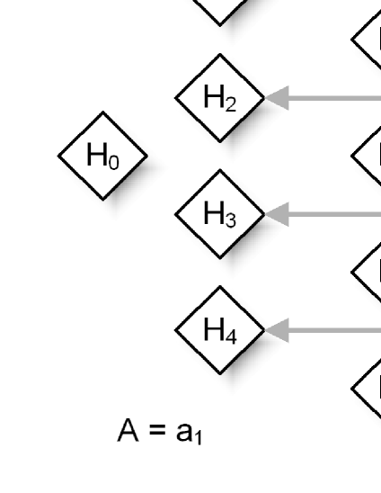
(a)	(b)

Figure 2: a. A graphical representation of combining factored transition and reward models (Figure 1b) with the linear approximation (Figure 1c). Reward nodes $G_{0}$ and $G_{i}$ ($i\geq 1$) represent the discounted backprojection terms $-\gamma w_{0}$ and $-\gamma w_{i}x_{i}^{\prime}$ ($i\geq 1$). Gray regions are the cost components of the constraint space. b. A cost network corresponding to our factored constraint space (Figure 2a). The network captures pairwise dependencies $X_{1}\!-\!X_{2}$, $X_{2}\!-\!X_{3}$, and $X_{3}\!-\!X_{4}$. The treewidth of the cost network is 1.

Inspired by the factorization, ? (?) proposed a variable-elimination method (?) that rewrites the constraint space in ALP compactly. ? (?) solved the same problem by the cutting plane method. The method iteratively searches for the most violated constraint:

$$\arg\min_{{\bf x},a}\left[\sum_{i}w^{(t)}_{i}\bigg{[}f_{i}({\bf x}_{i})-\gamma\sum_{{\bf x}_{i}^{\prime}}P({\bf x}_{i}^{\prime}\mid{\bf x},a)f_{i}({\bf x}_{i}^{\prime})\bigg{]}-R({\bf x},a)\right]$$ (7)

with respect to the solution ${\bf w}^{(t)}$ of a relaxed ALP. The constraint is added to the LP, which is resolved for a new solution ${\bf w}^{(t+1)}$. This procedure is iterated until no violated constraint is found, so that ${\bf w}^{(t)}$ is an optimal solution to the ALP.

The quality of the ALP formulation has been studied by ? (?). Based on their work, we conclude that ALP yields a close approximation $V^{\widetilde{{\bf w}}}$ to the optimal value function $V^{\ast}$ if the weighted max-norm error $\left\|V^{\ast}-V^{\bf w}\right\|_{\infty,1/L}$ can be minimized. We return to this theoretical result in Section 5.1.

Theorem 1 (?)

Let $\widetilde{{\bf w}}$ be a solution to the ALP formulation (6). Then the expected error of the value function $V^{\widetilde{{\bf w}}}$ can be bounded as:

$$\left\|V^{\ast}-V^{\widetilde{{\bf w}}}\right\|_{1,\psi}\leq\frac{2\psi^{\mathsf{\scriptscriptstyle T}}L}{1-\kappa}\min_{\bf w}\left\|V^{\ast}-V^{\bf w}\right\|_{\infty,1/L},$$

where $\left\|\cdot\right\|_{1,\psi}$ is an $\mathcal{L}_{1}$-norm weighted by the state relevance weights $\psi$, $L({\bf x})\!=\!\sum_{i}w_{i}^{L}f_{i}({\bf x})$ is a Lyapunov function such that the inequality $\kappa L({\bf x})\geq\gamma\sup_{\bf a}\mathrm{E}_{P({\bf x}^{\prime}\mid{\bf x},{\bf a})}\!\left[L({\bf x}^{\prime})\right]$ holds, $\kappa\in[0,1)$ denotes its contraction factor, and $\left\|\cdot\right\|_{\infty,1/L}$ is a max-norm reweighted by the reciprocal $1/L$.

Note that the $\mathcal{L}_{1}$-norm distance $\left\|V^{\ast}-V^{\widetilde{{\bf w}}}\right\|_{1,\psi}$ equals to the expectation $\mathrm{E}_{\psi}\!\left|V^{\ast}-V^{\widetilde{{\bf w}}}\right|$ over the state space ${\bf X}$ with respect to the state relevance weights $\psi$. Similarly to Theorem 1, we utilize the $\mathcal{L}_{1}$ and $\mathcal{L}_{\infty}$ norms in the rest of the work to measure the expected and worst-case errors of value functions. These norms are defined as follows.

Definition 1

The $\mathcal{L}_{1}$ (Manhattan) and $\mathcal{L}_{\infty}$ (infinity) norms are typically defined as $\left\|f\right\|_{1}=\sum_{\bf x}\left|f({\bf x})\right|$ and $\left\|f\right\|_{\infty}=\max_{\bf x}\left|f({\bf x})\right|$. If the state space ${\bf X}$ is represented by both discrete and continuous variables ${\bf X}_{D}$ and ${\bf X}_{C}$, the definition of the norms changes accordingly:

$$\left\|f\right\|_{1}=\sum_{{\bf x}_{D}}\int_{{\bf x}_{C}}\!\!\!\left|f({\bf x})\right|\,\mathrm{d}{\bf x}_{C}\quad\emph{and}\quad\left\|f\right\|_{\infty}=\sup_{\bf x}\left|f({\bf x})\right|.$$ (8)

The following definitions:

$$\left\|f\right\|_{1,\psi}=\sum_{{\bf x}_{D}}\int_{{\bf x}_{C}}\!\!\!\psi({\bf x})\left|f({\bf x})\right|\,\mathrm{d}{\bf x}_{C}\quad\emph{and}\quad\left\|f\right\|_{\infty,\psi}=\sup_{\bf x}\psi({\bf x})\left|f({\bf x})\right|$$ (9)

correspond to the $\mathcal{L}_{1}$ and $\mathcal{L}_{\infty}$ norms reweighted by a function $\psi({\bf x})$.

4 Hybrid Factored MDPs

Discrete-state factored MDPs (Section 3) permit a compact representation of decision problems with discrete states. However, real-world domains often involve continuous quantities, such as temperature and pressure. A sufficient discretization of these quantities may require hundreds of points in a single dimension, which renders the representation of our transition model (Equation 4) infeasible. In addition, rough and uninformative discretization impacts the quality of policies. Therefore, we want to avoid discretization or defer it until necessary. As a step in this direction, we discuss a formalism for representing hybrid decision problems in the domains of discrete and continuous variables.

4.1 Factored Transition and Reward Models

A hybrid factored MDP (HMDP) is a 4-tuple $\mathcal{M}=({\bf X},{\bf A},P,R)$, where ${\bf X}=\left\{X_{1},\dots,X_{n}\right\}$ is a state space described by state variables, ${\bf A}=\left\{A_{1},\dots,A_{m}\right\}$ is an action space described by action variables, $P({\bf X}^{\prime}\mid{\bf X},{\bf A})$ is a stochastic transition model of state dynamics conditioned on the preceding state and action, and $R$ is a reward function assigning immediate payoffs to state-action configurations.

State variables: State variables are either discrete or continuous. Every discrete variable $X_{i}$ takes on values from a finite domain $\mathrm{Dom}(X_{i})$. Following ? (?), we assume that every continuous variable is bounded to the $[0,1]$ subspace. In general, this assumption is very mild and permits modeling of any closed interval on $\mathbb{R}$. The state of the system is completely observed and described by a vector of value assignments ${\bf x}=({\bf x}_{D},{\bf x}_{C})$ which partitions along its discrete and continuous components ${\bf x}_{D}$ and ${\bf x}_{C}$.

Action variables: The action space is distributed and represented by action variables ${\bf A}$. The composite action is defined by a vector of individual action choices ${\bf a}=({\bf a}_{D},{\bf a}_{C})$ which partitions along its discrete and continuous components ${\bf a}_{D}$ and ${\bf a}_{C}$.

Transition model: The transition model is given by the conditional probability distribution $P({\bf X}^{\prime}\mid{\bf X},{\bf A})$, where ${\bf X}$ and ${\bf X}^{\prime}$ denote the state variables at two successive time steps. We assume that this distribution factors along ${\bf X}^{\prime}$ as $P({\bf X}^{\prime}\mid{\bf X},{\bf A})=\prod_{i=1}^{n}P(X_{i}^{\prime}\mid\mathsf{Par}(X_{i}^{\prime}))$ and can be described compactly by a DBN (?). Typically, the parent set $\mathsf{Par}(X_{i}^{\prime})\subseteq{\bf X}\cup{\bf A}$ is a small subset of state and action variables which allows for a local parameterization of the transition model.

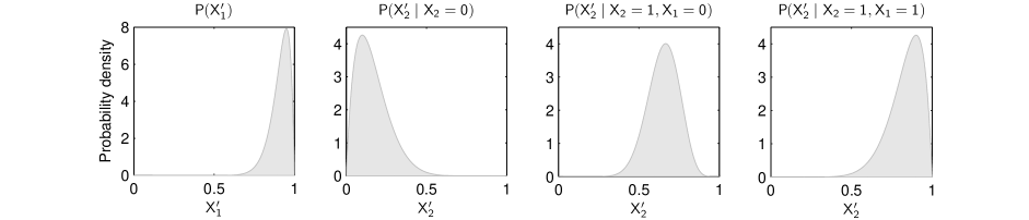
Figure 3: Transition functions for continuous variables $X_{1}^{\prime}$ and $X_{2}^{\prime}$ after taking an action $a_{1}$ in the 4-ring topology (Example 4). The densities are shown for extreme values of their parent variables $X_{1}$ and $X_{2}$.

Parameterization of our transition model: One-step dynamics of every state variable is described by its conditional probability distribution $P(X_{i}^{\prime}\mid\mathsf{Par}(X_{i}^{\prime}))$. If $X_{i}^{\prime}$ is a continuous variable, its transition function is represented by a mixture of beta distributions (?):

$$P(X_{i}^{\prime}=x\mid\mathsf{Par}(X_{i}^{\prime}))\ =\ \sum_{j}\pi_{ij}P_{\mathrm{beta}}(x\mid\alpha_{j},\beta_{j})$$ (10)

$$P_{\mathrm{beta}}(x\mid\alpha,\beta)\ =\ \frac{\Gamma(\alpha+\beta)}{\Gamma(\alpha)\Gamma(\beta)}x^{\alpha-1}(1-x)^{\beta-1},$$

where $\pi_{ij}$ is the weight assigned to the $j$-th component of the mixture, and $\alpha_{j}=\phi_{ij}^{\alpha}(\mathsf{Par}(X_{i}^{\prime}))$ and $\beta_{j}=\phi_{ij}^{\beta}(\mathsf{Par}(X_{i}^{\prime}))$ are arbitrary positive functions of the parent set. The mixture of beta distributions provides a very general class of transition functions and yet allows closed-form solutions to the expectation terms in HALP (Section 5). If every $\beta_{j}=1$, Equation 10 turns into a polynomial in $X_{i}^{\prime}$. Due to the Weierstrass approximation theorem (?), such a polynomial is sufficient to approximate any continuous transition density over $X_{i}^{\prime}$ with any precision. If $X_{i}^{\prime}$ is a discrete variable, its transition model is parameterized by $\left|\mathrm{Dom}(X_{i}^{\prime})\right|$ nonnegative discriminant functions $\theta_{j}=\phi_{ij}^{\theta}(\mathsf{Par}(X_{i}^{\prime}))$ (?):

$$P(X_{i}^{\prime}=j\mid\mathsf{Par}(X_{i}^{\prime}))=\frac{\theta_{j}}{\sum_{j=1}^{\left|\mathrm{Dom}(X_{i}^{\prime})\right|}\theta_{j}}.$$ (11)

Note that the parameters $\alpha_{j}$, $\beta_{j}$, and $\theta_{j}$ (Equations 10 and 11) are functions instantiated by value assignments to the variables $\mathsf{Par}(X_{i}^{\prime})\subseteq{\bf X}\cup{\bf A}$. We keep separate parameters for every state variable $X_{i}^{\prime}$ although our indexing does not reflect this explicitly. The only restriction on the functions is that they return valid parameters for all state-action pairs $({\bf x},{\bf a})$. Hence, we assume that $\alpha_{j}({\bf x},{\bf a})\geq 0$, $\beta_{j}({\bf x},{\bf a})\geq 0$, $\theta_{j}({\bf x},{\bf a})\geq 0$, and $\sum_{j=1}^{\left|\mathrm{Dom}(X_{i}^{\prime})\right|}\theta_{j}({\bf x},{\bf a})>0$.

Reward model: The reward model factors similarly to the transition model. In particular, the reward function $R({\bf x},{\bf a})=\sum_{j}R_{j}({\bf x}_{j},{\bf a}_{j})$ is an additive function of local reward functions defined on the subsets ${\bf X}_{j}$ and ${\bf A}_{j}$. In graphical models, the local functions can be described compactly by reward nodes $R_{j}$, which are conditioned on their parent sets $\mathsf{Par}(R_{j})\!=\!{\bf X}_{j}\cup{\bf A}_{j}$. To allow this representation, we formally extend our DBN to an influence diagram (?). Note that the form of the reward functions $R_{j}({\bf x}_{j},{\bf a}_{j})$ is not restricted.

Optimal value function and policy: The optimal policy $\pi^{\ast}$ can be defined greedily with respect to the optimal value function $V^{\ast}$, which is a fixed point of the Bellman equation:

$$V^{\ast}({\bf x})\ =\ \sup_{\bf a}\left[R({\bf x},{\bf a})+\gamma\mathrm{E}_{P({\bf x}^{\prime}\mid{\bf x},{\bf a})}\!\left[V^{\ast}({\bf x}^{\prime})\right]\right]$$ (12)

$$=\ \sup_{\bf a}\left[R({\bf x},{\bf a})+\gamma\sum_{{\bf x}_{D}^{\prime}}\int_{{\bf x}_{C}^{\prime}}\!\!\!P({\bf x}^{\prime}\mid{\bf x},{\bf a})V^{\ast}({\bf x}^{\prime})\,\mathrm{d}{\bf x}_{C}^{\prime}\right].$$

Accordingly, the hybrid Bellman operator $\mathcal{T}^{\ast}$ is given by:

$$\mathcal{T}^{\ast}V({\bf x})=\sup_{\bf a}\left[R({\bf x},{\bf a})+\gamma\mathrm{E}_{P({\bf x}^{\prime}\mid{\bf x},{\bf a})}\!\left[V({\bf x}^{\prime})\right]\right].$$ (13)

In the rest of the paper, we denote expectation terms over discrete and continuous variables in a unified form:

$$\mathrm{E}_{P({\bf x})}\!\left[f({\bf x})\right]=\sum_{{\bf x}_{D}}\int_{{\bf x}_{C}}P({\bf x})f({\bf x})\,\mathrm{d}{\bf x}_{C}.$$ (14)

Example 4 (?)

Continuous-state network administration is a variation on Example 1, where the computer states are represented by continuous variables on the interval between 0 (being down) and 1 (running). At each time step, the administrator selects a single action from the set $\mathcal{A}=\left\{a_{1},\dots,a_{n+1}\right\}$. The action $a_{i}$ ($i\leq n$) corresponds to rebooting the $i$-th computer. The last action $a_{n+1}$ is dummy. The transition model captures the propagation of failures in the network and is encoded locally by beta distributions:

$$P(X_{i}^{\prime}=x\mid\mathsf{Par}(X_{i}^{\prime}))=P_{\mathrm{beta}}(x\mid\alpha,\beta)\quad\begin{array}[]{|l l l}&\alpha=20&a=i\\ &\beta=2&\\ &\alpha=2+13x_{i}-5x_{i}\mathrm{E}\!\left[\mathsf{Par}(X_{i}^{\prime})\right]&a\neq i\\ &\beta=10-2x_{i}-6x_{i}\mathrm{E}\!\left[\mathsf{Par}(X_{i}^{\prime})\right]&\end{array}$$

where the variables $x_{i}$ and $\mathrm{E}\!\left[\mathsf{Par}(X_{i}^{\prime})\right]$ denote the state of the $i$-th computer and the expected state of its parents. Note that this transition function is similar to Example 1. For instance, in the 4-ring topology, the modes of transition densities for continuous variables $X_{1}^{\prime}$ and $X_{2}^{\prime}$ after taking an action $a_{1}$ (Figure 3):

$$\begin{array}[]{r r}\widehat{P}(X_{1}^{\prime}\mid a=a_{1})=0.95&\widehat{P}(X_{2}^{\prime}\mid X_{2}=1,X_{1}=0,a=a_{1})\approx 0.67\\ \widehat{P}(X_{2}^{\prime}\mid X_{2}=0,a=a_{1})=0.10&\widehat{P}(X_{2}^{\prime}\mid X_{2}=1,X_{1}=1,a=a_{1})=0.90\end{array}$$

equal to the expected values of their discrete counterparts (Figure 1b). The reward function is additive:

$$R({\bf x},a)=2x_{1}^{2}+\sum_{j=2}^{n}x_{j}^{2}$$

and establishes our preferences for maintaining the server $X_{1}$ and workstations $X_{2},\dots,X_{n}$.

4.2 Solving Hybrid Factored MDPs

Value iteration, policy iteration, and linear programming are the most fundamental dynamic programming methods for solving MDPs (?, ?). Unfortunately, none of these techniques is suitable for solving hybrid factored MDPs. First, their complexity is exponential in the number of state variables if the variables are discrete. Second, the methods assume a finite support for the optimal value function or policy, which may not exist if continuous variables are present. Therefore, any feasible approach to solving arbitrary HMDPs is likely to be approximate. In the rest of the section, we review two major classes of methods for approximating value functions in hybrid domains.

Grid-based approximation: Grid-based methods (?, ?) transform the initial state space ${\bf X}$ into a set of grid points $G=\left\{{\bf x}^{(1)},\dots,{\bf x}^{(N)}\right\}$. The points are used to estimate the optimal value function $V_{G}^{\ast}$ on the grid, which in turn approximates $V^{\ast}$. The Bellman operator on the grid is defined as (?):

$$\mathcal{T}_{G}^{\ast}V({\bf x}^{(i)})=\max_{\bf a}\left[R({\bf x}^{(i)},{\bf a})+\gamma\sum_{j=1}^{N}P_{G}({\bf x}^{(j)}\mid{\bf x}^{(i)},{\bf a})V({\bf x}^{(j)})\right],$$ (15)

where $P_{G}({\bf x}^{(j)}\mid{\bf x}^{(i)},{\bf a})=\Psi_{\bf a}^{-1}({\bf x}^{(i)})P({\bf x}^{(j)}\mid{\bf x}^{(i)},{\bf a})$ is a transition function, which is normalized by the term $\Psi_{\bf a}({\bf x}^{(i)})=\sum_{j=1}^{N}P({\bf x}^{(j)}\mid{\bf x}^{(i)},a)$. The operator $\mathcal{T}_{G}^{\ast}$ allows the computation of the value function $V_{G}^{\ast}$ by standard techniques for solving discrete-state MDPs.

? (?) analyzed the convergence of these methods for random and pseudo-random samples. Clearly, a uniform discretization of increasing precision guarantees the convergence of $V_{G}^{\ast}$ to $V^{\ast}$ but causes an exponential blowup in the state space (?). To overcome this concern, ? (?) proposed an adaptive algorithm for non-uniform discretization based on the Kuhn triangulation. ? (?) analyzed metrics for aggregating states in continuous-state MDPs based on the notion of bisimulation. ? (?) used linear programming to solve low-dimensional problems with continuous variables. These continuous variables were discretized manually.

Parametric value function approximation: An alternative approach to solving factored MDPs with continuous-state components is the approximation of the optimal value function $V^{\ast}$ by some parameterized model $V^{\lambda}$ (?, ?, ?). The parameters $\lambda$ are typically optimized iteratively by applying the backup operator $\mathcal{T}^{\ast}$ to a finite set of states. The least-squares error $\left\|V^{\lambda}-\mathcal{T}^{\ast}V^{\lambda}\right\|_{2}$ is a commonly minimized error metric (Figure 4). Online updating by gradient methods (?, ?) is another way of optimizing value functions. The limitation of these techniques is that their solutions are often unstable and may diverge (?). On the other hand, they generate high-quality approximations.

 

Inputs:
	a hybrid factored MDP $\mathcal{M}=({\bf X},{\bf A},P,R)$
	basis functions $f_{0}({\bf x}),f_{1}({\bf x}),f_{2}({\bf x}),\dots$
	initial basis function weights ${\bf w}^{(0)}$
	a set of states $G=\left\{{\bf x}^{(1)},\dots,{\bf x}^{(N)}\right\}$
Algorithm:
	$t=0$
	while a stopping criterion is not met
		for every state ${\bf x}^{(j)}$
			for every basis function $f_{i}({\bf x})$
				${\bf X}_{ji}=f_{i}({\bf x}^{(j)})$
			${\bf y}_{j}=\max_{\bf a}\left[R({\bf x}^{(j)},{\bf a})+\gamma\mathrm{E}_{P({\bf x}^{\prime}\mid{\bf x}^{(j)},{\bf a})}\!\left[V^{{\bf w}^{(t)}}({\bf x}^{\prime})\right]\right]$
		${\bf w}^{(t+1)}=({\bf X}^{\mathsf{\scriptscriptstyle T}}{\bf X})^{-1}{\bf X}^{\mathsf{\scriptscriptstyle T}}{\bf y}$
		$t=t+1$
Outputs:
	basis function weights ${\bf w}^{(t)}$

 

Figure 4: Pseudo-code implementation of the least-squares value iteration ($\mathcal{L}_{2}$ VI) with the linear value function approximation (Equation 5). The stopping criterion is often based on the number of steps or the $\mathcal{L}_{2}$-norm error $\left\|V^{{\bf w}^{(t)}}-\mathcal{T}^{\ast}V^{{\bf w}^{(t)}}\right\|_{2}$ measured on the set $G$. Our discussion in Sections 5.2 and 6 provides a recipe for an efficient implementation of the backup operation $\mathcal{T}^{\ast}V^{{\bf w}^{(t)}}({\bf x}^{(j)})$.

Parametric approximations often assume fixed value function models. However, in some cases, it is possible to derive flexible forms of $V^{\lambda}$ that combine well with the backup operator $\mathcal{T}^{\ast}$. For instance, ? (?) showed that convex piecewise linear functions are sufficient to represent value functions and their DP backups in partially-observable MDPs (POMDPs) (?, ?). Based on this idea, ? (?) proposed a method for solving MDPs with continuous variables. To obtain full DP backups, the value function approximation is restricted to rectangular piecewise linear and convex (RPWLC) functions. Further restrictions are placed on the transition and reward models of MDPs. The advantage of the approach is its adaptivity. The major disadvantages are restrictions on solved MDPs and the complexity of RPWLC value functions, which may grow exponentially in the number of backups. As a result, without further modifications, this approach is less likely to succeed in solving high-dimensional and distributed decision problems.

5 Hybrid Approximate Linear Programming

To overcome the limitations of existing methods for solving HMDPs (Section 4.2), we extend the discrete-state ALP (Section 3.3) to hybrid state and action spaces. We refer to this novel framework as hybrid approximate linear programming (HALP).

Similarly to the discrete-state ALP, HALP optimizes the linear value function approximation (Equation 5). Therefore, it transforms an initially intractable problem of computing $V^{\ast}$ in the hybrid state space ${\bf X}$ into a lower dimensional space of ${\bf w}$. The HALP formulation is given by a linear program:

$$\textrm{minimize}_{\bf w} \quad\sum_{i}w_{i}\alpha_{i}$$ (16)

subject to: $$\quad\sum_{i}w_{i}F_{i}({\bf x},{\bf a})-R({\bf x},{\bf a})\geq 0\quad\forall\ {\bf x}\in{\bf X},{\bf a}\in{\bf A};$$

where ${\bf w}$ represents the variables in the LP, $\alpha_{i}$ denotes basis function relevance weight:

$$\alpha_{i}\ =\ \mathrm{E}_{\psi({\bf x})}\!\left[f_{i}({\bf x})\right]$$ (17)

$$=\ \sum_{{\bf x}_{D}}\int_{{\bf x}_{C}}\!\!\!\psi({\bf x})f_{i}({\bf x})\,\mathrm{d}{\bf x}_{C},$$

$\psi({\bf x})\geq 0$ is a state relevance density function that weights the quality of the approximation, and $F_{i}({\bf x},{\bf a})=f_{i}({\bf x})-\gamma g_{i}({\bf x},{\bf a})$ denotes the difference between the basis function $f_{i}({\bf x})$ and its discounted backprojection:

$$g_{i}({\bf x},{\bf a})\ =\ \mathrm{E}_{P({\bf x}^{\prime}\mid{\bf x},{\bf a})}\!\left[f_{i}({\bf x}^{\prime})\right]$$ (18)

$$=\ \sum_{{\bf x}_{D}^{\prime}}\int_{{\bf x}_{C}^{\prime}}\!\!\!P({\bf x}^{\prime}\mid{\bf x},{\bf a})f_{i}({\bf x}^{\prime})\,\mathrm{d}{\bf x}_{C}^{\prime}.$$

Vectors ${\bf x}_{D}$ (${\bf x}_{D}^{\prime}$) and ${\bf x}_{C}$ (${\bf x}_{C}^{\prime}$) are the discrete and continuous components of value assignments ${\bf x}$ (${\bf x}^{\prime}$) to all state variables ${\bf X}$ (${\bf X}^{\prime}$). The linear program can be rewritten compactly:

$$\textrm{minimize}_{\bf w} \quad\mathrm{E}_{\psi}\!\left[V^{\bf w}\right]$$ (19)

subject to: $$\quad V^{\bf w}-\mathcal{T}^{\ast}V^{\bf w}\geq 0$$

by using the Bellman operator $\mathcal{T}^{\ast}$.

The HALP formulation reduces to the discrete-state ALP (Section 3.3) if the state and action variables are discrete, and to the continuous-state ALP (?) if the state variables are continuous. The formulation is feasible if the set of basis functions contains a constant function $f_{0}({\bf x})\equiv 1$. We assume that such a basis function is present.

In the rest of the paper, we address several concerns related to the HALP formulation. First, we analyze the quality of this approximation and relate it to the minimization of the max-norm error $\left\|V^{\ast}-V^{\bf w}\right\|_{\infty}$, which is a commonly-used metric (Section 5.1). Second, we present rich classes of basis functions that lead to closed-form solutions to the expectation terms in the objective function and constraints (Equations 17 and 18). These terms involve sums and integrals over the complete state space ${\bf X}$ (Section 5.2), and therefore are hard to evaluate. Finally, we discuss approximations to the constraint space in HALP and introduce a framework for solving HALP formulations in a unified way (Section 6). Note that complete satisfaction of this constraint space may not be possible since every state-action pair $({\bf x},{\bf a})$ induces a constraint.

5.1 Error Bounds

The quality of the ALP approximation (Section 3.3) has been studied by ? (?). We follow up on their work and extend it to structured state and action spaces with continuous variables. Before we proceed, we demonstrate that a solution to the HALP formulation (16) constitutes an upper bound on the optimal value function $V^{\ast}$.

Proposition 1

Let $\widetilde{{\bf w}}$ be a solution to the HALP formulation (16). Then $V^{\widetilde{{\bf w}}}\geq V^{\ast}$.

This result allows us to restate the objective $\mathrm{E}_{\psi}\!\left[V^{\bf w}\right]$ in HALP.

Proposition 2

Vector $\widetilde{{\bf w}}$ is a solution to the HALP formulation (16):

$$\emph{{minimize}}_{\bf w} \quad\mathrm{E}_{\psi}\!\left[V^{\bf w}\right]$$

subject to: $$\quad V^{\bf w}-\mathcal{T}^{\ast}V^{\bf w}\geq 0$$

if and only if it solves:

$$\emph{{minimize}}_{\bf w} \quad\left\|V^{\ast}-V^{\bf w}\right\|_{1,\psi}$$

subject to: $$\quad V^{\bf w}-\mathcal{T}^{\ast}V^{\bf w}\geq 0;$$

where $\left\|\cdot\right\|_{1,\psi}$ is an $\mathcal{L}_{1}$-norm weighted by the state relevance density function $\psi$ and $\mathcal{T}^{\ast}$ is the hybrid Bellman operator.

Based on Proposition 2, we conclude that HALP optimizes the linear value function approximation with respect to the reweighted $\mathcal{L}_{1}$-norm error $\left\|V^{\ast}-V^{\bf w}\right\|_{1,\psi}$. The following theorem draws a parallel between minimizing this objective and max-norm error $\left\|V^{\ast}-V^{\bf w}\right\|_{\infty}$. More precisely, the theorem says that HALP yields a close approximation $V^{\widetilde{{\bf w}}}$ to the optimal value function $V^{\ast}$ if $V^{\ast}$ is close to the span of basis functions $f_{i}({\bf x})$.

Theorem 2

Let $\widetilde{{\bf w}}$ be an optimal solution to the HALP formulation (16). Then the expected error of the value function $V^{\widetilde{{\bf w}}}$ can be bounded as:

$$\left\|V^{\ast}-V^{\widetilde{{\bf w}}}\right\|_{1,\psi}\leq\frac{2}{1-\gamma}\min_{\bf w}\left\|V^{\ast}-V^{\bf w}\right\|_{\infty},$$

where $\left\|\cdot\right\|_{1,\psi}$ is an $\mathcal{L}_{1}$-norm weighted by the state relevance density function $\psi$ and $\left\|\cdot\right\|_{\infty}$ is a max-norm.

Unfortunately, Theorem 2 rarely yields a tight bound on $\left\|V^{\ast}-V^{\widetilde{{\bf w}}}\right\|_{1,\psi}$. First, it is hard to guarantee a uniformly low max-norm error $\left\|V^{\ast}-V^{\bf w}\right\|_{\infty}$ if the dimensionality of a problem grows but the basis functions $f_{i}({\bf x})$ are local. Second, the bound ignores the state relevance density function $\psi({\bf x})$ although this one impacts the quality of HALP solutions. To address these concerns, we introduce non-uniform weighting of the max-norm error in Theorem 3.

Theorem 3

Let $\widetilde{{\bf w}}$ be an optimal solution to the HALP formulation (16). Then the expected error of the value function $V^{\widetilde{{\bf w}}}$ can be bounded as:

$$\left\|V^{\ast}-V^{\widetilde{{\bf w}}}\right\|_{1,\psi}\leq\frac{2\mathrm{E}_{\psi}\!\left[L\right]}{1-\kappa}\min_{\bf w}\left\|V^{\ast}-V^{\bf w}\right\|_{\infty,1/L},$$

where $\left\|\cdot\right\|_{1,\psi}$ is an $\mathcal{L}_{1}$-norm weighted by the state relevance density $\psi$, $L({\bf x})\!=\!\sum_{i}w_{i}^{L}f_{i}({\bf x})$ is a Lyapunov function such that the inequality $\kappa L({\bf x})\geq\gamma\sup_{\bf a}\mathrm{E}_{P({\bf x}^{\prime}\mid{\bf x},{\bf a})}\!\left[L({\bf x}^{\prime})\right]$ holds, $\kappa\in[0,1)$ denotes its contraction factor, and $\left\|\cdot\right\|_{\infty,1/L}$ is a max-norm reweighted by the reciprocal $1/L$.

Note that Theorem 2 is a special form of Theorem 3 when $L({\bf x})\equiv 1$ and $\kappa=\gamma$. Therefore, the Lyapunov function $L({\bf x})$ permits at least as good bounds as Theorem 2. To make these bounds tight, the function $L({\bf x})$ should return large values in the regions of the state space, which are unimportant for modeling. In turn, the reciprocal $1/L({\bf x})$ is close to zero in these undesirable regions, which makes their impact on the max-norm error $\left\|V^{\ast}-V^{\bf w}\right\|_{\infty,1/L}$ less likely. Since the state relevance density function $\psi({\bf x})$ reflects the importance of states, the term $\mathrm{E}_{\psi}\!\left[L\right]$ should remain small. These two factors contribute to tighter bounds than those by Theorem 2.

Since the Lyapunov function $L({\bf x})=\sum_{i}w_{i}^{L}f_{i}({\bf x})$ lies in the span of basis functions $f_{i}({\bf x})$, Theorem 3 provides a recipe for achieving high-quality approximations. Intuitively, a good set of basis functions always involves two types of functions. The first type guarantees small errors $\left|V^{\ast}({\bf x})-V^{\bf w}({\bf x})\right|$ in the important regions of the state space, where the state relevance density $\psi({\bf x})$ is high. The second type returns high values where the state relevance density $\psi({\bf x})$ is low, and vice versa. The latter functions allow the satisfaction of the constraint space $V^{\bf w}\geq\mathcal{T}^{\ast}V^{\bf w}$ in the unimportant regions of the state space without impacting the optimized objective function $\left\|V^{\ast}-V^{\bf w}\right\|_{1,\psi}$. Note that a trivial value function $V^{\bf w}({\bf x})=(1-\gamma)^{-1}R_{\mathrm{max}}$ satisfies all constraints in any HALP but unlikely leads to good policies. For a comprehensive discussion on selecting appropriate $\psi({\bf x})$ and $L({\bf x})$, refer to the case studies of ? (?).

Our discussion is concluded by clarifying the notion of the state relevance density $\psi({\bf x})$. As demonstrated by Theorem 4, its choice is closely related to the quality of a greedy policy for the value function $V^{\widetilde{{\bf w}}}$ (?).

Theorem 4

Let $\widetilde{{\bf w}}$ be an optimal solution to the HALP formulation (16). Then the expected error of a greedy policy:

$$u({\bf x})=\arg\sup_{\bf a}\left[R({\bf x},{\bf a})+\gamma\mathrm{E}_{P({\bf x}^{\prime}\mid{\bf x},{\bf a})}\!\left[V^{\widetilde{{\bf w}}}({\bf x}^{\prime})\right]\right]$$

can be bounded as:

$$\left\|V^{\ast}-V^{u}\right\|_{1,\nu}\leq\frac{1}{1-\gamma}\left\|V^{\ast}-V^{\widetilde{{\bf w}}}\right\|_{1,\mu_{u,\nu}},$$

where $\left\|\cdot\right\|_{1,\nu}$ and $\left\|\cdot\right\|_{1,\mu_{u,\nu}}$ are weighted $\mathcal{L}_{1}$-norms, $V^{u}$ is a value function for the greedy policy $u$, and $\mu_{u,\nu}$ is the expected frequency of state visits generated by following the policy $u$ given the initial state distribution $\nu$.

Based on Theorem 4, we may conclude that the expected error of greedy policies for HALP approximations is bounded when $\psi\!=\!\mu_{u,\nu}$. Note that the distribution $\mu_{u,\nu}$ is unknown when optimizing $V^{\widetilde{{\bf w}}}$ because it is a function of the optimized quantity itself. To break this cycle, ? (?) suggested an iterative procedure that solves several LPs and adapts $\mu_{u,\nu}$ accordingly. In addition, real-world control problems exhibit a lot of structure, which permits the guessing of $\mu_{u,\nu}$.

Finally, it is important to realize that although our bounds (Theorems 3 and 4) build a foundation for better HALP approximations, they can be rarely used in practice because the optimal value function $V^{\ast}$ is generally unknown. After all, if it was known, there is no need to approximate it. Moreover, note that the optimization of $\left\|V^{\ast}-V^{\bf w}\right\|_{\infty,1/L}$ (Theorem 3) is a hard problem and there are no methods that would minimize this error directly (?). Despite these facts, both bounds provide a loose guidance for empirical choices of basis functions. In Section 7, we use this intuition and propose basis functions that should closely approximate unknown optimal value functions $V^{\ast}$.

5.2 Expectation Terms

Since our basis functions are often restricted to small subsets of state variables, expectation terms (Equations 17 and 18) in the HALP formulation (16) should be efficiently computable. To unify the analysis of these expectation terms, $\mathrm{E}_{\psi({\bf x})}\!\left[f_{i}({\bf x})\right]$ and $\mathrm{E}_{P({\bf x}^{\prime}\mid{\bf x},{\bf a})}\!\left[f_{i}({\bf x}^{\prime})\right]$, we show that their evaluation constitutes the same computational problem $\mathrm{E}_{P({\bf x})}\!\left[f_{i}({\bf x})\right]$, where $P({\bf x})$ denotes some factored distribution.

Before we discuss expectation terms in the constraints, note that the transition function $P({\bf x}^{\prime}\mid{\bf x},{\bf a})$ is factored and its parameterization is determined by the state-action pair $({\bf x},{\bf a})$. We keep the pair $({\bf x},{\bf a})$ fixed in the rest of the section, which corresponds to choosing a single constraint $({\bf x},{\bf a})$. Based on this selection, we rewrite the expectation terms $\mathrm{E}_{P({\bf x}^{\prime}\mid{\bf x},{\bf a})}\!\left[f_{i}({\bf x}^{\prime})\right]$ in a simpler notation $\mathrm{E}_{P({\bf x}^{\prime})}\!\left[f_{i}({\bf x}^{\prime})\right]$, where $P({\bf x}^{\prime})\!=\!P({\bf x}^{\prime}\!\mid\!{\bf x},{\bf a})$ denotes a factored distribution with fixed parameters.

We also assume that the state relevance density function $\psi({\bf x})$ factors along ${\bf X}$ as:

$$\psi({\bf x})=\prod_{i=1}^{n}\psi_{i}(x_{i}),$$ (20)

where $\psi_{i}(x_{i})$ is a distribution over the random state variable $X_{i}$. Based on this assumption, we can rewrite the expectation terms $\mathrm{E}_{\psi({\bf x})}\!\left[f_{i}({\bf x})\right]$ in the objective function in a new notation $\mathrm{E}_{P({\bf x})}\!\left[f_{i}({\bf x})\right]$, where $P({\bf x})=\psi({\bf x})$ denotes a factored distribution. In line with our discussion in the last two paragraphs, efficient solutions to the expectation terms in HALP are obtained by solving the generalized term $\mathrm{E}_{P({\bf x})}\!\left[f_{i}({\bf x})\right]$ efficiently. We address this problem in the rest of the section.

Before computing the expectation term $\mathrm{E}_{P({\bf x})}\!\left[f_{i}({\bf x})\right]$ over the complete state space ${\bf X}$, we recall that the basis function $f_{i}({\bf x})$ is defined on a subset of state variables ${\bf X}_{i}$. Therefore, we may conclude that $\mathrm{E}_{P({\bf x})}\!\left[f_{i}({\bf x})\right]=\mathrm{E}_{P({\bf x}_{i})}\!\left[f_{i}({\bf x}_{i})\right]$, where $P({\bf x}_{i})$ denotes a factored distribution on a lower dimensional space ${\bf X}_{i}$. If no further assumptions are made, the local expectation term $\mathrm{E}_{P({\bf x}_{i})}\!\left[f_{i}({\bf x}_{i})\right]$ may be still hard to compute. Although it can be estimated by a variety of numerical methods, for instance Monte Carlo (?), these techniques are imprecise if the sample size is small, and quite computationally expensive if a high precision is needed. Consequently, we try to avoid such an approximation step. Instead, we introduce an appropriate form of basis functions that leads to closed-form solutions to the expectation term $\mathrm{E}_{P({\bf x}_{i})}\!\left[f_{i}({\bf x}_{i})\right]$.

In particular, let us assume that every basis function $f_{i}({\bf x}_{i})$ factors as:

$$f_{i}({\bf x}_{i})=f_{i_{D}}({\bf x}_{i_{D}})f_{i_{C}}({\bf x}_{i_{C}})$$ (21)

along its discrete and continuous components $f_{i_{D}}({\bf x}_{i_{D}})$ and $f_{i_{C}}({\bf x}_{i_{C}})$, where the continuous component further decouples as a product:

$$f_{i_{C}}({\bf x}_{i_{C}})=\prod_{X_{j}\in{\bf X}_{i_{C}}}f_{ij}(x_{j})$$ (22)

of univariate basis function factors $f_{ij}(x_{j})$. Note that the basis functions remain multivariate despite the two independence assumptions. We make these presumptions for computational purposes and they are relaxed later in the section.

Based on Equation 21, we conclude that the expectation term:

$$\mathrm{E}_{P({\bf x}_{i})}\!\left[f_{i}({\bf x}_{i})\right]\ =\ \mathrm{E}_{P({\bf x}_{i})}\!\left[f_{i_{D}}({\bf x}_{i_{D}})f_{i_{C}}({\bf x}_{i_{C}})\right]$$

$$=\ \mathrm{E}_{P({\bf x}_{i_{D}})}\!\left[f_{i_{D}}({\bf x}_{i_{D}})\right]\mathrm{E}_{P({\bf x}_{i_{C}})}\!\left[f_{i_{C}}({\bf x}_{i_{C}})\right]$$ (23)

decomposes along the discrete and continuous variables ${\bf X}_{i_{D}}$ and ${\bf X}_{i_{C}}$, where ${\bf x}_{i}=({\bf x}_{i_{D}},{\bf x}_{i_{C}})$ and $P({\bf x}_{i})=P({\bf x}_{i_{D}})P({\bf x}_{i_{C}})$. The evaluation of the discrete part $\mathrm{E}_{P({\bf x}_{i_{D}})}\!\left[f_{i_{D}}({\bf x}_{i_{D}})\right]$ requires aggregation in the subspace ${\bf X}_{i_{D}}$:

$$\mathrm{E}_{P({\bf x}_{i_{D}})}\!\left[f_{i_{D}}({\bf x}_{i_{D}})\right]=\sum_{{\bf x}_{i_{D}}}P({\bf x}_{i_{D}})f_{i_{D}}({\bf x}_{i_{D}}),$$ (24)

which can be carried out efficiently in $O(\prod_{X_{j}\in{\bf X}_{i_{D}}}\left|\mathrm{Dom}(X_{j})\right|)$ time (Section 3.3). Following Equation 22, the continuous term $\mathrm{E}_{P({\bf x}_{i_{C}})}\!\left[f_{i_{C}}({\bf x}_{i_{C}})\right]$ decouples as a product:

$$\mathrm{E}_{P({\bf x}_{i_{C}})}\!\left[f_{i_{C}}({\bf x}_{i_{C}})\right]\ =\ \mathrm{E}_{P({\bf x}_{i_{C}})}\!\left[\prod_{X_{j}\in{\bf X}_{i_{C}}}f_{ij}(x_{j})\right]$$

$$=\ \prod_{X_{j}\in{\bf X}_{i_{C}}}\mathrm{E}_{P(x_{j})}\!\left[f_{ij}(x_{j})\right],$$ (25)

where $\mathrm{E}_{P(x_{j})}\!\left[f_{ij}(x_{j})\right]$ represents the expectation terms over individual random variables $X_{j}$. Consequently, an efficient solution to the local expectation term $\mathrm{E}_{P({\bf x}_{i})}\!\left[f_{i}({\bf x}_{i})\right]$ is guaranteed by efficient solutions to its univariate components $\mathrm{E}_{P(x_{j})}\!\left[f_{ij}(x_{j})\right]$.

In this paper, we consider three univariate basis function factors $f_{ij}(x_{j})$: piecewise linear functions, polynomials, and beta distributions. These factors support a very general class of basis functions and yet allow closed-form solutions to the expectation terms $\mathrm{E}_{P(x_{j})}\!\left[f_{ij}(x_{j})\right]$. These solutions are provided in the following propositions and demonstrated in Example 5.

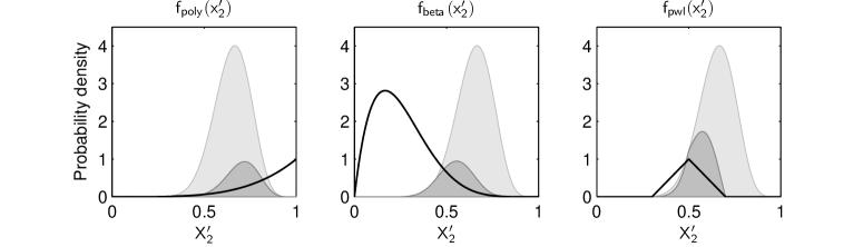
Figure 5: Expectation of three basis functions $f(x_{2}^{\prime})$ (Example 5) with respect to the transition function $P(X_{2}^{\prime}\mid X_{2}=1,X_{1}=0,a=a_{1})$ from Figure 3. Every basis function $f(x_{2}^{\prime})$ is depicted by a thick black line. The transition function is shown in a light gray color. Darker gray lines represent the values of the product $P(x_{2}^{\prime}\!\mid\!{\bf x},a_{1})f(x_{2}^{\prime})$. The area below corresponds to the expectation terms $\mathrm{E}_{P(x_{2}^{\prime}\mid{\bf x},a_{1})}\!\left[f(x_{2}^{\prime})\right]$.

Proposition 3 (Polynomial basis functions)

Let:

$$P(x)=P_{\mathrm{beta}}(x\mid\alpha,\beta)$$

be a beta distribution over $X$ and:

$$f(x)=x^{n}(1-x)^{m}$$

be a polynomial in $x$ and $(1-x)$. Then $\mathrm{E}_{P(x)}\!\left[f(x)\right]$ has a closed-form solution:

$$\mathrm{E}_{P(x)}\!\left[f(x)\right]=\frac{\Gamma(\alpha+\beta)}{\Gamma(\alpha)\Gamma(\beta)}\frac{\Gamma(\alpha+n)\Gamma(\beta+m)}{\Gamma(\alpha+\beta+n+m)}.$$

Corollary 1 (Beta basis functions)

Let:

$$P(x)\ =\ P_{\mathrm{beta}}(x\mid\alpha,\beta)$$

$$f(x)\ =\ P_{\mathrm{beta}}(x\mid\alpha_{f},\beta_{f})$$

be beta distributions over $X$. Then $\mathrm{E}_{P(x)}\!\left[f(x)\right]$ has a closed-form solution:

$$\mathrm{E}_{P(x)}\!\left[f(x)\right]=\frac{\Gamma(\alpha+\beta)}{\Gamma(\alpha)\Gamma(\beta)}\frac{\Gamma(\alpha_{f}+\beta_{f})}{\Gamma(\alpha_{f})\Gamma(\beta_{f})}\frac{\Gamma(\alpha+\alpha_{f}-1)\Gamma(\beta+\beta_{f}-1)}{\Gamma(\alpha+\alpha_{f}+\beta+\beta_{f}-2)}.$$

Proof: A direct consequence of Proposition 3. Since integration is a distributive operation, our claim straightforwardly generalizes to the mixture of beta distributions $P(x)$. $\square$

Proposition 4 (Piecewise linear basis functions)

Let:

$$P(x)=P_{\mathrm{beta}}(x\mid\alpha,\beta)$$

be a beta distribution over $X$ and:

$$f(x)=\sum_{i}\mathbf{1}_{[l_{i},r_{i}]}(x)(a_{i}x+b_{i})$$

be a piecewise linear (PWL) function in $x$, where $\mathbf{1}_{[l_{i},r_{i}]}(x)$ represents the indicator function of the interval $[l_{i},r_{i}]$. Then $\mathrm{E}_{P(x)}\!\left[f(x)\right]$ has a closed-form solution:

$$\mathrm{E}_{P(x)}\!\left[f(x)\right]=\sum_{i}\left[a_{i}\frac{\alpha}{\alpha+\beta}(F^{+}(r_{i})-F^{+}(l_{i}))+b_{i}(F(r_{i})-F(l_{i}))\right],$$

where $F(u)=F_{\mathrm{beta}}(u\mid\alpha,\beta)$ and $F^{+}(u)=F_{\mathrm{beta}}(u\mid\alpha+1,\beta)$ denote the cumulative density functions of beta distributions.

Example 5

Efficient closed-form solutions to the expectation terms in HALP are illustrated on the 4-ring network administration problem (Example 4) with three hypothetical univariate basis functions:

$$f_{\mathrm{poly}}(x_{2}^{\prime})\ =\ x_{2}^{\prime 4}$$

$$f_{\mathrm{beta}}(x_{2}^{\prime})\ =\ P_{\mathrm{beta}}(x_{2}^{\prime}\mid 2,6)$$

$$f_{\mathrm{pwl}}(x_{2}^{\prime})\ =\ \mathbf{1}_{[0.3,0.5]}(x_{2}^{\prime})(5x_{2}^{\prime}-1.5)+\mathbf{1}_{[0.5,0.7]}(x_{2}^{\prime})(-5x_{2}^{\prime}+3.5)$$

Suppose that our goal is to evaluate expectation terms in a single constraint that corresponds to the network state ${\bf x}\!=\!(0,1,0,0)$ and the administrator rebooting the server. Based on these assumptions, the expectation terms in the constraint $({\bf x},a_{1})$ simplify as:

$$\mathrm{E}_{P({\bf x}^{\prime}\mid{\bf x},a_{1})}\!\left[f(x_{2}^{\prime})\right]=\mathrm{E}_{P(x_{2}^{\prime}\mid{\bf x},a_{1})}\!\left[f(x_{2}^{\prime})\right],$$

where the transition function $P(x_{2}^{\prime}\mid{\bf x},a_{1})$ is given by:

$$P(x_{2}^{\prime}\mid{\bf x},a_{1})\ =\ P(X_{2}^{\prime}=x_{2}^{\prime}\mid X_{2}=1,X_{1}=0,a=a_{1})$$

$$=\ P_{\mathrm{beta}}(x_{2}^{\prime}\mid 15,8).$$

Closed-form solutions to the simplified expectation terms $\mathrm{E}_{P(x_{2}^{\prime}\mid{\bf x},a_{1})}\!\left[f(x_{2}^{\prime})\right]$ are computed as:

$$\mathrm{E}_{P(x_{2}^{\prime}\mid{\bf x},a_{1})}\!\left[f_{\mathrm{poly}}(x_{2}^{\prime})\right]\ = \ \ \int_{x_{2}^{\prime}}P_{\mathrm{beta}}(x_{2}^{\prime}\mid 15,8)x_{2}^{\prime 4}\,\mathrm{d}x_{2}^{\prime}$$

$${\scriptstyle\emph{(Proposition \ref{prop:polynomial basis function})}}\ = \ \ \frac{\Gamma(15+8)}{\Gamma(15)\Gamma(8)}\frac{\Gamma(15+4)\Gamma(8)}{\Gamma(15+8+4)}$$

$$\approx \ \ 0.20$$

$$\mathrm{E}_{P(x_{2}^{\prime}\mid{\bf x},a_{1})}\!\left[f_{\mathrm{beta}}(x_{2}^{\prime})\right]\ = \ \ \int_{x_{2}^{\prime}}P_{\mathrm{beta}}(x_{2}^{\prime}\mid 15,8)P_{\mathrm{beta}}(x_{2}^{\prime}\mid 2,6)\,\mathrm{d}x_{2}^{\prime}$$

$${\scriptstyle\emph{(Corollary \ref{cor:beta basis function})}}\ = \ \ \frac{\Gamma(15+8)}{\Gamma(15)\Gamma(8)}\frac{\Gamma(2+6)}{\Gamma(2)\Gamma(6)}\frac{\Gamma(15+2-1)\Gamma(8+6-1)}{\Gamma(15+2+8+6-2)}$$

$$\approx \ \ 0.22$$

$$\mathrm{E}_{P(x_{2}^{\prime}\mid{\bf x},a_{1})}\!\left[f_{\mathrm{pwl}}(x_{2}^{\prime})\right]\ = \ \ \int_{x_{2}^{\prime}}P_{\mathrm{beta}}(x_{2}^{\prime}\mid 15,8)\mathbf{1}_{[0.3,0.5]}(x_{2}^{\prime})(5x_{2}^{\prime}-1.5)\,\mathrm{d}x_{2}^{\prime}+$$

$$\ \ \int_{x_{2}^{\prime}}P_{\mathrm{beta}}(x_{2}^{\prime}\mid 15,8)\mathbf{1}_{[0.5,0.7]}(x_{2}^{\prime})(-5x_{2}^{\prime}+3.5)\,\mathrm{d}x_{2}^{\prime}$$

$${\scriptstyle\emph{(Proposition \ref{prop:piecewise linear basis function})}}\ = \ \ 5\frac{15}{15+8}(F^{+}(0.5)-F^{+}(0.3))-1.5(F(0.5)-F(0.3))-$$

$$\ \ 5\frac{15}{15+8}(F^{+}(0.7)-F^{+}(0.5))+3.5(F(0.7)-F(0.5))$$

$$\approx \ \ 0.30$$

where $F(u)=F_{\mathrm{beta}}(u\mid 15,8)$ and $F^{+}(u)=F_{\mathrm{beta}}(u\mid 15+1,8)$ denote the cumulative density functions of beta distributions. A graphical interpretation of these computations is presented in Figure 5. Brief inspection verifies that the term $\mathrm{E}_{P(x_{2}^{\prime}\mid{\bf x},a_{1})}\!\left[f_{\mathrm{pwl}}(x_{2}^{\prime})\right]$ is indeed the largest one.

Up to this point, we obtained efficient closed-form solutions for factored basis functions and state relevance densities. Unfortunately, the factorization assumptions in Equations 20, 21, and 22 are rarely justified in practice. In the rest of the section, we show how to relax them. In Section 6, we apply our current results and propose several methods that approximately satisfy the constraint space in HALP.

5.2.1 Factored State Relevance Density Functions

Note that the state relevance density function $\psi({\bf x})$ is very unlikely to be completely factored (Section 5.1). Therefore, the independence assumption in Equation 20 is extremely limiting. To relax this assumption, we approximate $\psi({\bf x})$ by a linear combination $\psi^{\omega}({\bf x})\!=\!\sum_{\ell}\omega_{\ell}\psi_{\ell}({\bf x})$ of factored state relevance densities $\psi_{\ell}({\bf x})=\prod_{i=1}^{n}\psi_{\ell i}(x_{i})$. As a result, the expectation terms in the objective function decompose as:

$$\mathrm{E}_{\psi^{\omega}({\bf x})}\!\left[f_{i}({\bf x})\right]\ =\ \mathrm{E}_{\sum_{\ell}\omega_{\ell}\psi_{\ell}({\bf x})}\!\left[f_{i}({\bf x})\right]$$

$$=\ \sum_{\ell}\omega_{\ell}\mathrm{E}_{\psi_{\ell}({\bf x})}\!\left[f_{i}({\bf x})\right],$$ (26)

where the factored terms $\mathrm{E}_{\psi_{\ell}({\bf x})}\!\left[f_{i}({\bf x})\right]$ can be evaluated efficiently (Equation 23). Moreover, if we assume the factored densities $\psi_{\ell}({\bf x})$ are polynomials, their linear combination $\psi^{\omega}({\bf x})$ is a polynomial. Due to the Weierstrass approximation theorem (?), this polynomial is sufficient to approximate any state relevance density $\psi({\bf x})$ with any precision. It follows that the linear combinations permit state relevance densities that reflect arbitrary dependencies among the state variables ${\bf X}$.

5.2.2 Factored Basis Functions

In line with the previous discussion, note that the linear value function $V^{\bf w}({\bf x})=\sum_{i}w_{i}f_{i}({\bf x})$ with factored basis functions (Equations 21 and 22) is sufficient to approximate the optimal value function $V^{\ast}$ within any max-norm error $\left\|V^{\ast}-V^{\bf w}\right\|_{\infty}$. Based on Theorem 2, we know that the same set of basis functions guarantees a bound on the $\mathcal{L}_{1}$-norm error $\left\|V^{\ast}-V^{\widetilde{{\bf w}}}\right\|_{1,\psi}$. Therefore, despite our independence assumptions (Equations 21 and 22), we have a potential to obtain an arbitrarily close HALP approximation $V^{\widetilde{{\bf w}}}$ to $V^{\ast}$.

6 Constraint Space Approximations

An optimal solution $\widetilde{{\bf w}}$ to the HALP formulation (16) is determined by a finite set of active constraints at a vertex of the feasible region. Unfortunately, identification of this active set is a hard computational problem. In particular, it requires searching through an exponential number of constraints, if the state and action variables are discrete, and an infinite number of constraints, if any of the variables are continuous. As a result, it is in general infeasible to find the optimal solution $\widetilde{{\bf w}}$ to the HALP formulation. Hence, we resort to approximations to the constraint space in HALP whose optimal solution $\widehat{{\bf w}}$ is close to $\widetilde{{\bf w}}$. This notion of an approximation is formalized as follows.

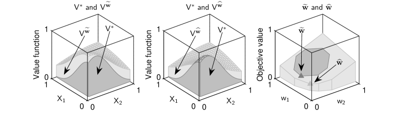
(a)                             (b)                             (c)

Figure 6: a. Graphical relation between the value function $V^{\ast}$ and its HALP approximation $V^{\widetilde{{\bf w}}}$. The function $V^{\widetilde{{\bf w}}}$ is guaranteed to be an upper bound on $V^{\ast}$. b. The relaxed HALP approximation $V^{\widehat{{\bf w}}}$ may not lead to an upper bound. c. Graphical relation between the optimal and relaxed solutions $\widetilde{{\bf w}}$ and $\widehat{{\bf w}}$. The feasible regions of the complete and relaxed HALP formulations are shown in dark and light gray colors. The value function approximations $V^{\widetilde{{\bf w}}}$ and $V^{\widehat{{\bf w}}}$ are typically nonlinear in the state space ${\bf X}$ but always linear in the space of parameters ${\bf w}$.

Definition 2

The HALP formulation is relaxed:

$$\emph{{minimize}}_{\bf w} \quad\sum_{i}w_{i}\alpha_{i}$$ (27)

subject to: $$\quad\sum_{i}w_{i}F_{i}({\bf x},{\bf a})-R({\bf x},{\bf a})\geq 0\quad({\bf x},{\bf a})\in\mathcal{C};$$

if only a subset $\mathcal{C}$ of its constraints is satisfied.

The HALP formulation (16) can be solved approximately by solving its relaxed formulations (27). Several methods for building and solving these approximate LPs have been proposed: Monte Carlo sampling of constraints, (?), $\varepsilon$-grid discretization of the constraint space (?), and an adaptive search for a violated constraint (?). In the remainder of this section, we introduce these methods. From now on, we denote optimal solutions to the complete and relaxed HALP formulations by the symbols $\widetilde{{\bf w}}$ and $\widehat{{\bf w}}$, respectively.

Before we proceed, note that while $V^{\widetilde{{\bf w}}}$ is an upper bound on the optimal value function $V^{\ast}$ (Figure 6a), the relaxed value function $V^{\widehat{{\bf w}}}$ does not have to be (Figure 6b). The reason is that the relaxed HALP formulation does not guarantee that the constraint $V^{\widehat{{\bf w}}}\geq\mathcal{T}^{\ast}V^{\widehat{{\bf w}}}$ is satisfied for all states ${\bf x}$. As a result, we cannot simply use Proposition 1 to prove $V^{\widehat{{\bf w}}}\geq V^{\ast}$. Furthermore, note that the inequality $\mathrm{E}_{\psi}\!\left[V^{\widehat{{\bf w}}}\right]\leq\mathrm{E}_{\psi}\!\left[V^{\widetilde{{\bf w}}}\right]$ always holds because the optimal solution $\widetilde{{\bf w}}$ is feasible in the relaxed HALP (Figure 6c). These observations become helpful for understanding the rest of the section.

6.1 MC-HALP

In the simplest case, the constraint space in HALP can be approximated by its Monte Carlo (MC) sample. In such a relaxation, the set of constraints $\mathcal{C}$ is selected with respect to some proposal distribution $\varphi$ over state-action pairs $({\bf x},{\bf a})$. Since the set $\mathcal{C}$ is finite, it establishes a relaxed formulation (27), which can be solved by any LP solver. An algorithm that builds and satisfies relaxed MC-HALP formulations is outlined in Figure 7.

Constraint sampling is easily applied in continuous domains and its space complexity is proportional to the number of state and action components. ? (?) used it to solve continuous-state factored MDPs and further refined it by heuristics (?). In discrete-state domains, the quality of the sampled approximations was analyzed by ? (?). Their result is summarized by Theorem 5.

Theorem 5 (?)

Let $\widetilde{{\bf w}}$ be a solution to the ALP formulation (6) and $\widehat{{\bf w}}$ be a solution to its relaxed formulation whose constraints are sampled with respect to a proposal distribution $\varphi$ over state-action pairs $({\bf x},{\bf a})$. Then there exist a distribution $\varphi$ and sample size:

$$N\geq O\left(\frac{A\theta}{(1-\gamma)\epsilon}\left(K\ln\frac{A\theta}{(1-\gamma)\epsilon}+\ln\frac{1}{\delta}\right)\right)$$

such that with probability at least $1-\delta$:

$$\left\|V^{\ast}-V^{\widehat{{\bf w}}}\right\|_{1,\psi}\leq\left\|V^{\ast}-V^{\widetilde{{\bf w}}}\right\|_{1,\psi}+\epsilon\left\|V^{\ast}\right\|_{1,\psi},$$

where $\left\|\cdot\right\|_{1,\psi}$ is an $\mathcal{L}_{1}$-norm weighted by the state relevance weights $\psi$, $\theta$ is a problem-specific constant, $A$ and $K$ denote the numbers of actions and basis functions, and $\epsilon$ and $\delta$ are scalars from the interval $(0,1)$.

Unfortunately, proposing a sampling distribution $\varphi$ that guarantees this polynomial bound on the sample size is as hard as knowing the optimal policy $\pi^{\ast}$ (?). This conclusion is parallel to those in importance sampling. Note that uniform Monte Carlo sampling can guarantee a low probability of constraints being violated but it is not sufficient to bound the magnitude of their violation (?).

6.2 $\varepsilon$-HALP

 

Inputs:
	a hybrid factored MDP $\mathcal{M}=({\bf X},{\bf A},P,R)$
	basis functions $f_{0}({\bf x}),f_{1}({\bf x}),f_{2}({\bf x}),\dots$
	a proposal distribution $\varphi$
Algorithm:
	initialize a relaxed HALP formulation with an empty set of constraints
	$t=0$
	while a stopping criterion is not met
		sample $({\bf x},{\bf a})\sim\varphi$
		add the constraint $({\bf x},{\bf a})$ to the relaxed HALP
		$t=t+1$
	solve the relaxed MC-HALP formulation
Outputs:
	basis function weights ${\bf w}$

 

Figure 7: Pseudo-code implementation of the MC-HALP solver.

 

Inputs:
	a hybrid factored MDP $\mathcal{M}=({\bf X},{\bf A},P,R)$
	basis functions $f_{0}({\bf x}),f_{1}({\bf x}),f_{2}({\bf x}),\dots$
	grid resolution $\varepsilon$
Algorithm:
	discretize continuous variables ${\bf X}_{C}$ and ${\bf A}_{C}$ into $\left\lceil 1/\varepsilon+1\right\rceil$ equally-spaced values
	identify subsets ${\bf X}_{i}$ and ${\bf A}_{i}$ (${\bf X}_{j}$ and ${\bf A}_{j}$) corresponding to the domains of $F_{i}({\bf x},{\bf a})$ ($R_{j}({\bf x},{\bf a})$)
	evaluate $F_{i}({\bf x}_{i},{\bf a}_{i})$ ($R_{j}({\bf x}_{j},{\bf a}_{j})$) for all configurations ${\bf x}_{i}$ and ${\bf a}_{i}$ (${\bf x}_{j}$ and ${\bf a}_{j}$) on the $\varepsilon$-grid
	calculate basis function relevance weights $\alpha_{i}$
	solve the relaxed $\varepsilon$-HALP formulation (Section 3.3)
Outputs:
	basis function weights ${\bf w}$

 

Figure 8: Pseudo-code implementation of the $\varepsilon$-HALP solver.

Another way of approximating the constraint space in HALP is by discretizing its continuous variables ${\bf X}_{C}$ and ${\bf A}_{C}$ on a uniform $\varepsilon$-grid. The new discretized constraint space preserves its original factored structure but spans discrete variables only. Therefore, it can be compactly satisfied by the methods for discrete-state ALP (Section 3.3). An algorithm that builds and satisfies relaxed $\varepsilon$-HALP formulations is outlined in Figure 8. Note that the new constraint space involves exponentially many constraints $O(\left\lceil 1/\varepsilon+1\right\rceil^{\left|{\bf X}_{C}\right|+\left|{\bf A}_{C}\right|})$ in the number of state and action variables ${\bf X}_{C}$ and ${\bf A}_{C}$.

6.2.1 Error Bounds

Recall that the $\varepsilon$-HALP formulation approximates the constraint space in HALP by a finite set of equally-spaced grid points. In this section, we study the quality of this approximation and bound it in terms violating constraints in the complete HALP. More precisely, we prove that if a relaxed HALP solution $\widehat{{\bf w}}$ violates the constraints in the complete HALP by a small amount, the quality of the approximation $V^{\widehat{{\bf w}}}$ is close to $V^{\widetilde{{\bf w}}}$. In the next section, we extend this result and relate $V^{\widehat{{\bf w}}}$ to the grid resolution $\varepsilon$. Before we proceed, we quantify our notion of constraint violation.

Definition 3

Let $\widehat{{\bf w}}$ be an optimal solution to a relaxed HALP formulation (27). The vector $\widehat{{\bf w}}$ is $\delta$-infeasible if:

$$V^{\widehat{{\bf w}}}-\mathcal{T}^{\ast}V^{\widehat{{\bf w}}}\geq-\delta,$$ (28)

where $\mathcal{T}^{\ast}$ is the hybrid Bellman operator.

Intuitively, the lower the $\delta$-infeasibility of a relaxed HALP solution $\widehat{{\bf w}}$, the closer the quality of the approximation $V^{\widehat{{\bf w}}}$ to $V^{\widetilde{{\bf w}}}$. Proposition 5 states this intuition formally. In particular, it says that the relaxed HALP formulation leads to a close approximation $V^{\widehat{{\bf w}}}$ to the optimal value function $V^{\ast}$ if the complete HALP does and the solution $\widehat{{\bf w}}$ violates its constraints by a small amount.

Proposition 5

Let $\widetilde{{\bf w}}$ be an optimal solution to the HALP formulation (16) and $\widehat{{\bf w}}$ be an optimal $\delta$-infeasible solution to its relaxed formulation (27). Then the expected error of the value function $V^{\widehat{{\bf w}}}$ can be bounded as:

$$\left\|V^{\ast}-V^{\widehat{{\bf w}}}\right\|_{1,\psi}\leq\left\|V^{\ast}-V^{\widetilde{{\bf w}}}\right\|_{1,\psi}+\frac{2\delta}{1-\gamma},$$

where $\left\|\cdot\right\|_{1,\psi}$ is an $\mathcal{L}_{1}$-norm weighted by the state relevance density function $\psi$.

Based on Proposition 5, we can generalize our conclusions from Section 5.1 to relaxed HALP formulations. For instance, we may draw a parallel between optimizing the relaxed objective $\mathrm{E}_{\psi}\!\left[V^{\widehat{{\bf w}}}\right]$ and the max-norm error $\left\|V^{\ast}-V^{\bf w}\right\|_{\infty,1/L}$.

Theorem 6

Let $\widehat{{\bf w}}$ be an optimal $\delta$-infeasible solution to a relaxed HALP formulation (27). Then the expected error of the value function $V^{\widehat{{\bf w}}}$ can be bounded as:

$$\left\|V^{\ast}-V^{\widehat{{\bf w}}}\right\|_{1,\psi}\leq\frac{2\mathrm{E}_{\psi}\!\left[L\right]}{1-\kappa}\min_{\bf w}\left\|V^{\ast}-V^{\bf w}\right\|_{\infty,1/L}+\frac{2\delta}{1-\gamma},$$

where $\left\|\cdot\right\|_{1,\psi}$ is an $\mathcal{L}_{1}$-norm weighted by the state relevance density $\psi$, $L({\bf x})\!=\!\sum_{i}w_{i}^{L}f_{i}({\bf x})$ is a Lyapunov function such that the inequality $\kappa L({\bf x})\geq\gamma\sup_{\bf a}\mathrm{E}_{P({\bf x}^{\prime}\mid{\bf x},{\bf a})}\!\left[L({\bf x}^{\prime})\right]$ holds, $\kappa\in[0,1)$ denotes its contraction factor, and $\left\|\cdot\right\|_{\infty,1/L}$ is a max-norm reweighted by the reciprocal $1/L$.

Proof: Direct combination of Theorem 3 and Proposition 5. $\square$

6.2.2 Grid Resolution

In Section 6.2.1, we bounded the error of a relaxed HALP formulation by its $\delta$-infeasibility (Theorem 6), a measure of constraint violation in the complete HALP. However, it is unclear how the grid resolution $\varepsilon$ relates to $\delta$-infeasibility. In this section, we analyze the relationship between $\varepsilon$ and $\delta$. Moreover, we show how to exploit the factored structure in the constraint space to achieve the $\delta$-infeasibility of a relaxed HALP solution $\widehat{{\bf w}}$ efficiently.

First, let us assume that $\widehat{{\bf w}}$ is an optimal $\delta$-infeasible solution to an $\varepsilon$-HALP formulation and ${\bf Z}={\bf X}\cup{\bf A}$ is the joint set of state and action variables. To derive a bound relating both $\varepsilon$ and $\delta$, we assume that the magnitudes of constraint violations $\tau^{\widehat{{\bf w}}}({\bf z})=\sum_{i}\widehat{w}_{i}F_{i}({\bf z})-R({\bf z})$ are Lipschitz continuous.

Definition 4

The function $f({\bf x})$ is Lipschitz continuous if:

$$\left|f({\bf x})-f({\bf x}^{\prime})\right|\leq K\left\|{\bf x}-{\bf x}^{\prime}\right\|_{\infty}\quad\forall\ {\bf x},{\bf x}^{\prime}\in{\bf X};$$ (29)

where $K$ is referred to as a Lipschitz constant.

Based on the $\varepsilon$-grid discretization of the constraint space, we know that the distance of any point ${\bf z}$ to its closest grid point ${\bf z}_{G}=\arg\min_{{\bf z}^{\prime}}\left\|{\bf z}-{\bf z}^{\prime}\right\|_{\infty}$ is bounded as:

$$\left\|{\bf z}-{\bf z}_{G}\right\|_{\infty}<\frac{\varepsilon}{2}.$$ (30)

From the Lipschitz continuity of $\tau^{\widehat{{\bf w}}}({\bf z})$, we conclude:

$$\left|\tau^{\widehat{{\bf w}}}({\bf z}_{G})-\tau^{\widehat{{\bf w}}}({\bf z})\right|\leq K\left\|{\bf z}_{G}-{\bf z}\right\|_{\infty}\leq\frac{K\varepsilon}{2}.$$ (31)

Since every constraint in the relaxed $\varepsilon$-HALP formulation is satisfied, $\tau^{\widehat{{\bf w}}}({\bf z}_{G})$ is nonnegative for all grid points ${\bf z}_{G}$. As a result, Equation 31 yields $\tau^{\widehat{{\bf w}}}({\bf z})>-K\varepsilon/2$ for every state-action pair ${\bf z}=({\bf x},{\bf a})$. Therefore, based on Definition 3, the solution $\widehat{{\bf w}}$ is $\delta$-infeasible for $\delta\geq K\varepsilon/2$. Conversely, the $\delta$-infeasibility of $\widehat{{\bf w}}$ is guaranteed by choosing $\varepsilon\leq 2\delta/K$.

Unfortunately, $K$ may increase rapidly with the dimensionality of a function. To address this issue, we use the structure in the constraint space and demonstrate that this is not our case. First, we observe that the global Lipschitz constant $K_{\mathrm{glob}}$ is additive in local Lipschitz constants that correspond to the terms $\widehat{w}_{i}F_{i}({\bf z})$ and $R_{j}({\bf z})$. Moreover, $K_{\mathrm{glob}}\leq NK_{\mathrm{loc}}$, where $N$ denotes the total number of the terms and $K_{\mathrm{loc}}$ is the maximum over the local constants. Finally, parallel to Equation 31, the $\delta$-infeasibility of a relaxed HALP solution $\widehat{{\bf w}}$ is achieved by the discretization:

$$\varepsilon\leq\frac{2\delta}{NK_{\mathrm{loc}}}\leq\frac{2\delta}{K_{\mathrm{glob}}}.$$ (32)

Since the factors $\widehat{w}_{i}F_{i}({\bf z})$ and $R_{j}({\bf z})$ are often restricted to small subsets of state and action variables, $K_{\mathrm{loc}}$ should change a little when the size of a problem increases but its structure is fixed. To prove that $K_{\mathrm{loc}}$ is bounded, we have to bound the weights $\widehat{w}_{i}$. If all basis functions are of unit magnitude, the weights $\widehat{w}_{i}$ are intuitively bounded as $\left|\widehat{w}_{i}\right|\leq(1-\gamma)^{-1}R_{\mathrm{max}}$, where $R_{\mathrm{max}}$ denotes the maximum one-step reward in the HMDP.

Based on Equation 32, we conclude that the number of discretization points in a single dimension $\left\lceil 1/\varepsilon+1\right\rceil$ is bounded by a polynomial in $N$, $K_{\mathrm{loc}}$, and $1/\delta$. Hence, the constraint space in the relaxed $\varepsilon$-HALP formulation involves $O([NK_{\mathrm{loc}}(1/\delta)]^{\left|{\bf X}\right|+\left|{\bf A}\right|})$ constraints, where $\left|{\bf X}\right|$ and $\left|{\bf A}\right|$ denote the number of state and action variables. The idea of variable elimination can be used to write the constraints compactly by $O([NK_{\mathrm{loc}}(1/\delta)]^{T+1}(\left|{\bf X}\right|+\left|{\bf A}\right|))$ constraints (Example 3), where $T$ is the treewidth of a corresponding cost network. Therefore, satisfying this constraint space is polynomial in $N$, $K_{\mathrm{loc}}$, $1/\delta$, $\left|{\bf X}\right|$, and $\left|{\bf A}\right|$, but still exponential in $T$.

6.3 Cutting Plane Method

 

Inputs:
	a hybrid factored MDP $\mathcal{M}=({\bf X},{\bf A},P,R)$
	basis functions $f_{0}({\bf x}),f_{1}({\bf x}),f_{2}({\bf x}),\dots$
	initial basis function weights ${\bf w}^{(0)}$
	a separation oracle $\mathcal{O}$
Algorithm:
	initialize a relaxed HALP formulation with an empty set of constraints
	$t=0$
	while a stopping criterion is not met
		query the oracle $\mathcal{O}$ for a violated constraint $({\bf x}_{\mathcal{O}},{\bf a}_{\mathcal{O}})$ with respect to ${\bf w}^{(t)}$
		if the constraint $({\bf x}_{\mathcal{O}},{\bf a}_{\mathcal{O}})$ is violated
			add the constraint to the relaxed HALP
		resolve the LP for a new vector ${\bf w}^{(t+1)}$
		$t=t+1$
Outputs:
	basis function weights ${\bf w}^{(t)}$

 

Figure 9: Pseudo-code implementation of a HALP solver with the cutting plane method.

Both MC and $\varepsilon$-HALP formulations (Sections 6.1 and 6.2) approximate the constraint space in HALP by a finite set of constraints $\mathcal{C}$. Therefore, they can be solved directly by any linear programming solver. However, if the number of constraints is large, formulating and solving LPs with the complete set of constraints is infeasible. In this section, we show how to build relaxed HALP approximations efficiently by the cutting plane method.

The cutting plane method for solving HALP formulations is outlined in Figure 9. Briefly, this approach builds the set of LP constraints incrementally by adding a violated constraint to this set in every step. In the remainder of the paper, we refer to any method that returns a violated constraint for an arbitrary vector $\widehat{{\bf w}}$ as a separation oracle. Formally, every HALP oracle approaches the optimization problem:

$$\arg\min_{{\bf x},{\bf a}}\left[V^{\widehat{{\bf w}}}({\bf x})-\gamma\mathrm{E}_{P({\bf x}^{\prime}\mid{\bf x},{\bf a})}\!\left[V^{\widehat{{\bf w}}}({\bf x}^{\prime})\right]-R({\bf x},{\bf a})\right].$$ (33)

Consequently, the problem of solving hybrid factored MDPs efficiently reduces to the design of efficient separation oracles. Note that the cutting plane method (Figure 9) can be applied to suboptimal solutions to Equation 33 if these correspond to violated constraints.

 

Inputs:
	a hybrid factored MDP $\mathcal{M}=({\bf X},{\bf A},P,R)$
	basis functions $f_{0}({\bf x}),f_{1}({\bf x}),f_{2}({\bf x}),\dots$
	basis function weights ${\bf w}$
	grid resolution $\varepsilon$
Algorithm:
	discretize continuous variables ${\bf X}_{C}$ and ${\bf A}_{C}$ into ($\left\lceil 1/\varepsilon+1\right\rceil$) equally-spaced values
	identify subsets ${\bf X}_{i}$ and ${\bf A}_{i}$ (${\bf X}_{j}$ and ${\bf A}_{j}$) corresponding to the domains of $F_{i}({\bf x},{\bf a})$ ($R_{j}({\bf x},{\bf a})$)
	evaluate $F_{i}({\bf x}_{i},{\bf a}_{i})$ ($R_{j}({\bf x}_{j},{\bf a}_{j})$) for all configurations ${\bf x}_{i}$ and ${\bf a}_{i}$ (${\bf x}_{j}$ and ${\bf a}_{j}$) on the $\varepsilon$-grid
	build a cost network for the factored cost function:
		$\tau^{\bf w}({\bf x},{\bf a})=\sum_{i}w_{i}F_{i}({\bf x},{\bf a})-R({\bf x},{\bf a})$
	find the most violated constraint in the cost network:
		$({\bf x}_{\mathcal{O}},{\bf a}_{\mathcal{O}})=\arg\min_{{\bf x},{\bf a}}\tau^{\bf w}({\bf x},{\bf a})$
Outputs:
	state-action pair $({\bf x}_{\mathcal{O}},{\bf a}_{\mathcal{O}})$

 

Figure 10: Pseudo-code implementation of the $\varepsilon$-HALP separation oracle $\mathcal{O}_{\varepsilon}$.

The presented approach can be directly used to satisfy the constraints in relaxed $\varepsilon$-HALP formulations (?). Briefly, the solver from Figure 9 iterates until no violated constraint is found and the $\varepsilon$-HALP separation oracle $\mathcal{O}_{\varepsilon}$ (Figure 10) returns the most violated constraint in the discretized cost network given an intermediate solution ${\bf w}^{(t)}$. Note that although the search for the most violated constraint is polynomial in $\left|{\bf X}\right|$ and $\left|{\bf A}\right|$ (Section 6.2.2), the running time of our solver does not have to be (?). In fact, the number of generated cuts is exponential in $\left|{\bf X}\right|$ and $\left|{\bf A}\right|$ in the worst case. However, the same oracle embedded into the ellipsoid method (?) yields a polynomial-time algorithm (?). Although this technique is impractical for solving large LPs, we may conclude that our approach is indeed polynomial-time if implemented in this particular way.

Finally, note that searching for the most violated constraint (Equation 33) has application beyond satisfying the constraint space in HALP. For instance, computation of a greedy policy for the value function $V^{\widehat{{\bf w}}}$:

$$u({\bf x})\ =\ \arg\max_{\bf a}\left[R({\bf x},{\bf a})+\gamma\mathrm{E}_{P({\bf x}^{\prime}\mid{\bf x},{\bf a})}\!\left[V^{\widehat{{\bf w}}}({\bf x}^{\prime})\right]\right]$$

$$=\ \arg\min_{\bf a}\left[-R({\bf x},{\bf a})-\gamma\mathrm{E}_{P({\bf x}^{\prime}\mid{\bf x},{\bf a})}\!\left[V^{\widehat{{\bf w}}}({\bf x}^{\prime})\right]\right]$$ (34)

is almost an identical optimization problem, where the state variables ${\bf X}$ are fixed. Moreover, the magnitude of the most violated constraint is equal to the lowest $\delta$ for which the relaxed HALP solution $\widehat{{\bf w}}$ is $\delta$-infeasible (Equation 28):

$$\underline{\delta}\ =\ \min_{\bf x}\left[V^{\widehat{{\bf w}}}({\bf x})-\max_{\bf a}\left[R({\bf x},{\bf a})+\gamma\mathrm{E}_{P({\bf x}^{\prime}\mid{\bf x},{\bf a})}\!\left[V^{\widehat{{\bf w}}}({\bf x}^{\prime})\right]\right]\right]$$

$$=\ \min_{{\bf x},{\bf a}}\left[V^{\widehat{{\bf w}}}({\bf x})-R({\bf x},{\bf a})-\gamma\mathrm{E}_{P({\bf x}^{\prime}\mid{\bf x},{\bf a})}\!\left[V^{\widehat{{\bf w}}}({\bf x}^{\prime})\right]\right].$$ (35)

6.4 MCMC-HALP

In practice, both MC and $\varepsilon$-HALP formulations (Sections 6.1 and 6.2) are built on a blindly selected set of constraints $\mathcal{C}$. More specifically, the constraints in the MC-HALP formulation are chosen randomly (with respect to a prior distribution $\varphi$) while the $\varepsilon$-HALP formulation is based on a uniform $\varepsilon$-grid. This discretized constraint space preserves its original factored structure, which allows for its compact satisfaction. However, the complexity of solving the $\varepsilon$-HALP formulation is exponential in the treewidth of its discretized constraint space. Note that if the discretized constraint space is represented by binary variables only, the treewidth increases by a multiplicative factor of $\log_{2}\left\lceil 1/\varepsilon+1\right\rceil$, where $\left\lceil 1/\varepsilon+1\right\rceil$ denotes the number of discretization points in a single dimension. Consequently, even if the treewidth of a problem is relatively small, solving its $\varepsilon$-HALP formulation becomes intractable for small values of $\varepsilon$.

To address the issues of the discussed approximations (Sections 6.1 and 6.2), we propose a novel Markov chain Monte Carlo (MCMC) method for finding the most violated constraint of a relaxed HALP. The procedure directly operates in the domains of continuous variables, takes into account the structure of factored MDPs, and its space complexity is proportional to the number of variables. This separation oracle can be easily embedded into the ellipsoid or cutting plane method for solving linear programs (Section 6.3), and therefore constitutes a key step towards solving HALP efficiently. Before we proceed, we represent the constraint space in HALP compactly and state an optimization problem for finding violated constraints in this factored representation.

6.4.1 Compact Representation of Constraints

In Section 3.3, we showed how the factored representation of the constraint space allows for its compact satisfaction. Following this idea, we define violation magnitude $\tau^{{\bf w}}({\bf x},{\bf a})$:

$$\tau^{\bf w}({\bf x},{\bf a})\ =\ -\left[V^{\bf w}({\bf x})-\gamma\mathrm{E}_{P({\bf x}^{\prime}\mid{\bf x},{\bf a})}\!\left[V^{\bf w}({\bf x}^{\prime})\right]-R({\bf x},{\bf a})\right]$$ (36)

$$=\ -\sum_{i}w_{i}[f_{i}({\bf x})-\gamma g_{i}({\bf x},{\bf a})]+R({\bf x},{\bf a}),$$

which measures the amount by which the solution ${\bf w}$ violates the constraints in the complete HALP. We represent the magnitude of violation $\tau^{{\bf w}}({\bf x},{\bf a})$ compactly by an influence diagram (ID), where ${\bf X}$ and ${\bf A}$ are decision nodes, and ${\bf X}^{\prime}$ are random variables. This representation is built on the transition model $P({\bf X}^{\prime}\mid{\bf X},{\bf A})$, which is factored and captures independencies among the variables ${\bf X}$, ${\bf X}^{\prime}$, and ${\bf A}$. We extend the diagram by three types of reward nodes, one for each term in Equation 36: $H_{i}=-w_{i}f_{i}({\bf x})$ for every basis function, $G_{i}=\gamma w_{i}f_{i}({\bf x}^{\prime})$ for every backprojection, and $R_{j}=R_{j}({\bf x}_{j},{\bf a}_{j})$ for every local reward function. The construction is completed by adding arcs that graphically represent the dependencies of the reward nodes on the variables. Finally, we can verify that:

$$\tau^{\bf w}({\bf x},{\bf a})=\mathrm{E}_{P({\bf x}^{\prime}\mid{\bf x},{\bf a})}\!\left[\sum_{i}(H_{i}+G_{i})+\sum_{j}R_{j}\right].$$ (37)

Consequently, the decision that maximizes the expected utility in the ID corresponds to the most violated constraint. A graphical representation of the violation magnitude $\tau^{{\bf w}}({\bf x},{\bf a})$ on the 4-ring network administration problem (Example 4) is given in Figure 2a. The structure of the constraint space is identical to Example 3 if the basis functions are univariate.

We conclude that any algorithm for solving IDs can be applied to find the most violated constraint. However, most of these methods (?, ?, ?) are restricted to discrete variables. Fortunately, special properties of the ID representation allow its further simplification. If the basis functions are chosen conjugate to the transition model (Section 5.2), we obtain a closed-form solution to the expectation term $\mathrm{E}_{P({\bf x}^{\prime}\mid{\bf x},{\bf a})}\!\left[G_{i}\right]$ (Equation 18), and the random variables ${\bf X}^{\prime}$ are marginalized out of the diagram. The new representation contains no random variables and is known as a cost network (Section 3.3).

Note that the problem of finding the most violated constraint in the ID representation is also identical to finding the maximum a posteriori (MAP) configuration of random variables in Bayesian networks (?, ?, ?, ?). The latter problem is difficult because of the alternating summation and maximization operators. Since we marginalized out the random variables ${\bf X}^{\prime}$, we can solve the maximization problem by standard large-scale optimization techniques.

6.4.2 Separation Oracle $\mathcal{O}_{\mathrm{MCMC}}$

To find the most violated constraint in the cost network, we apply the Metropolis-Hastings (MH) algorithm (?, ?) and propose a Markov chain whose invariant distribution converges to the vicinity of $\arg\max_{\bf z}\tau^{\bf w}({\bf z})$, where ${\bf z}=({\bf x},{\bf a})$ is a value assignment to the joint set of state and action variables ${\bf Z}={\bf X}\cup{\bf A}$.

In short, the Metropolis-Hastings algorithm defines a Markov chain that transits between an existing state ${\bf z}$ and a proposed state ${\bf z}^{\ast}$ with the acceptance probability:

$$A({\bf z},{\bf z}^{\ast})=\min\left\{1,\frac{p({\bf z}^{\ast})q({\bf z}\mid{\bf z}^{\ast})}{p({\bf z})q({\bf z}^{\ast}\mid{\bf z})}\right\},$$ (38)

where $q({\bf z}^{\ast}\mid{\bf z})$ and $p({\bf z})$ are a proposal distribution and a target density, respectively. Under mild restrictions on $p({\bf z})$ and $q({\bf z}^{\ast}\mid{\bf z})$, the frequency of state visits generated by the Markov chain always converges to the target function $p({\bf z})$ (?). In the remainder of this section, we discuss the choices of $p({\bf z})$ and $q({\bf z}^{\ast}\mid{\bf z})$ to solve our optimization problem.

Target density: The violation magnitude $\tau^{\bf w}({\bf z})$ is turned into a density by the transformation $p({\bf z})=\exp[\tau^{\bf w}({\bf z})]$. Due to its monotonic character, $p({\bf z})$ retains the same set of global maxima as $\tau^{\bf w}({\bf z})$. Therefore, the search for $\arg\max_{\bf z}\tau^{\bf w}({\bf z})$ can be done on the new function $p({\bf z})$. To prove that $p({\bf z})$ is a density, we demonstrate that $\sum_{{\bf z}_{D}}\int_{{\bf z}_{C}}p({\bf z})\,\mathrm{d}{\bf z}_{C}$ is a normalizing constant, where ${\bf z}_{D}$ and ${\bf z}_{C}$ are the discrete and continuous parts of the value assignment ${\bf z}$. First, note that the integrand ${\bf z}_{C}$ is restricted to the space $[0,1]^{\left|{\bf Z}_{C}\right|}$. As a result, the integral $\int_{{\bf z}_{C}}p({\bf z})\,\mathrm{d}{\bf z}_{C}$ is proper if $p({\bf z})$ is bounded, and hence it is Riemann integrable and finite. To prove that $p({\bf z})=\exp[\tau^{\bf w}({\bf z})]$ is bounded, we bound the magnitude of violation $\tau^{\bf w}({\bf z})$. If all basis functions are of unit magnitude, the weights $\widehat{w}_{i}$ can be bounded as $\left|\widehat{w}_{i}\right|\!\leq\!(1-\gamma)^{-1}R_{\mathrm{max}}$ (Section 6.2.2), which in turn yields the bound $\left|\tau^{\bf w}({\bf z})\right|\leq(\left|{\bf w}\right|(1-\gamma)^{-1}+1)R_{\mathrm{max}}$. Therefore, $p({\bf z})$ is bounded and can be treated as a density function.

To find the mode of $p({\bf z})$, we employ simulating annealing (?) and generate a non-homogeneous Markov chain whose invariant distribution is equal to $p^{1/T_{t}}({\bf z})$, where $T_{t}$ is a cooling schedule such that $\lim_{t\rightarrow\infty}T_{t}=0$. Under weak regularity assumptions on $p({\bf z})$, $p^{\infty}({\bf z})$ is a probability density that concentrates on the set of the global maxima of $p({\bf z})$ (?). If our cooling schedule $T_{t}$ decreases such that $T_{t}\geq c/\ln(t+1)$, where $c$ is a problem-specific constant, the chain from Equation 38 converges to the vicinity of $\arg\max_{\bf z}\tau^{\bf w}({\bf z})$ with the probability converging to 1 (?). However, this logarithmic cooling schedule is slow in practice, especially for a high initial temperature $c$. To overcome this problem, we select a smaller value of $c$ (?) than is required by the convergence criterion. Therefore, the convergence of our chain to the global optimum $\arg\max_{\bf z}\tau^{\bf w}({\bf z})$ is no longer guaranteed.

 

Inputs:
	a hybrid factored MDP $\mathcal{M}=({\bf X},{\bf A},P,R)$
	basis functions $f_{0}({\bf x}),f_{1}({\bf x}),f_{2}({\bf x}),\dots$
	basis function weights ${\bf w}$
Algorithm:
	initialize a state-action pair ${\bf z}^{(t)}$
	$t=0$
	while a stopping criterion is not met
		for every variable $Z_{i}$
			sample $u\sim\mathrm{U}_{[0,1]}$
			sample $z_{i}^{\ast}\sim p(Z_{i}\mid{\bf z}_{-i}^{(t)})$
			if $u<\min\left\{1,\frac{p^{1/T_{t}-1}(z_{i}^{\ast}\mid{\bf z}_{-i}^{(t)})}{p^{1/T_{t}-1}(z_{i}^{(t)}\mid{\bf z}_{-i}^{(t)})}\right\}$
				$z_{i}^{(t+1)}=z_{i}^{\ast}$
			else
				$z_{i}^{(t+1)}=z_{i}^{(t)}$
		update $T_{t+1}$ according to the cooling schedule
		$t=t+1$
	$({\bf x}_{\mathcal{O}},{\bf a}_{\mathcal{O}})={\bf z}^{(t)}$
Outputs:
	state-action pair $({\bf x}_{\mathcal{O}},{\bf a}_{\mathcal{O}})$

 

Figure 11: Pseudo-code implementation of the MCMC-HALP oracle $\mathcal{O}_{\mathrm{MCMC}}$. The symbol $\mathrm{U}_{[0,1]}$ denotes the uniform distribution on the interval $[0,1]$. Since the testing for violated constraints (Figure 9) is inexpensive, our implementation of the MCMC-HALP solver in Section 7 tests all constraints ${\bf z}^{(t)}$ generated by the Markov chain and not only the last one. Therefore, the separation oracle $\mathcal{O}_{\mathrm{MCMC}}$ returns more than one constraint per chain.

Proposal distribution: We take advantage of the factored character of ${\bf Z}$ and adopt the following proposal distribution (?):

$$q({\bf z}^{\ast}\mid{\bf z})=\left\{\begin{array}[]{l l}p(z^{\ast}_{i}\mid{\bf z}_{-i})&\mathrm{\hbox{if }}{\bf z}^{\ast}_{-i}={\bf z}_{-i}\\ 0&\mathrm{otherwise}\end{array}\right.,$$ (41)

where ${\bf z}_{-i}$ and ${\bf z}^{\ast}_{-i}$ are value assignments to all variables but $Z_{i}$ in the original and proposed states. If $Z_{i}$ is a discrete variable, its conditional:

$$p(z_{i}^{\ast}\mid{\bf z}_{-i})=\frac{p(z_{1},\dots,z_{i-1},z_{i}^{\ast},z_{i+1},\dots,z_{n+m})}{\sum_{z_{i}}p(z_{1},\dots,z_{i-1},z_{i},z_{i+1},\dots,z_{n+m})}$$ (42)

can be derived in a closed form. If $Z_{i}$ is a continuous variable, a closed form of its cumulative density function is unlikely to exist. To sample from the conditional, we embed another MH step within the original chain. In the experimental section, we use the Metropolis algorithm with the acceptance probability:

$$A(z_{i},z_{i}^{\ast})=\min\left\{1,\frac{p(z_{i}^{\ast}\mid{\bf z}_{-i})}{p(z_{i}\mid{\bf z}_{-i})}\right\},$$ (43)

where $z_{i}$ and $z_{i}^{\ast}$ are the original and proposed values of the variable $Z_{i}$. Note that sampling from both conditionals can be performed in the space of $\tau^{\bf w}({\bf z})$ and locally.

Finally, by assuming that ${\bf z}^{\ast}_{-i}={\bf z}_{-i}$ (Equation 41), we derive a non-homogenous Markov chain with the acceptance probability:

$$A({\bf z},{\bf z}^{\ast})\ =\ \min\left\{1,\frac{p^{1/T_{t}}({\bf z}^{\ast})q({\bf z}\mid{\bf z}^{\ast})}{p^{1/T_{t}}({\bf z})q({\bf z}^{\ast}\mid{\bf z})}\right\}$$

$$=\ \min\left\{1,\frac{p^{1/T_{t}}(z^{\ast}_{i}\mid{\bf z}^{\ast}_{-i})p^{1/T_{t}}({\bf z}^{\ast}_{-i})p(z_{i}\mid{\bf z}^{\ast}_{-i})}{p^{1/T_{t}}(z_{i}\mid{\bf z}_{-i})p^{1/T_{t}}({\bf z}_{-i})p(z^{\ast}_{i}\mid{\bf z}_{-i})}\right\}$$

$$=\ \min\left\{1,\frac{p^{1/T_{t}}(z^{\ast}_{i}\mid{\bf z}_{-i})p^{1/T_{t}}({\bf z}_{-i})p(z_{i}\mid{\bf z}_{-i})}{p^{1/T_{t}}(z_{i}\mid{\bf z}_{-i})p^{1/T_{t}}({\bf z}_{-i})p(z^{\ast}_{i}\mid{\bf z}_{-i})}\right\}$$

$$=\ \min\left\{1,\frac{p^{1/T_{t}-1}(z_{i}^{\ast}\mid{\bf z}_{-i})}{p^{1/T_{t}-1}(z_{i}\mid{\bf z}_{-i})}\right\},$$ (44)

which converges to the vicinity of the most violated constraint. ? (?) proposed a similar chain for finding the MAP configuration of random variables in Bayesian networks.

6.4.3 Constraint Satisfaction

If the MCMC-HALP separation oracle $\mathcal{O}_{\mathrm{MCMC}}$ (Figure 11) converges to a violated constraint (not necessarily the most violated) in polynomial time, the ellipsoid method is guaranteed to solve HALP formulations in polynomial time (?). Unfortunately, convergence of our chain within arbitrary precision requires an exponential number of steps (?). Although the bound is loose to be of practical interest, it suggests that the time complexity of proposing violated constraints dominates the time complexity of solving relaxed HALP formulations. Therefore, the oracle $\mathcal{O}_{\mathrm{MCMC}}$ should search for violated constraints efficiently. Convergence speedups that directly apply to our work include hybrid Monte Carlo (HMC) (?), Rao-Blackwellization (?), and slice sampling (?).

7 Experiments

Experimental section is divided in three parts. First, we show that HALP can solve a simple HMDP problem at least as efficiently as alternative approaches. Second, we demonstrate the scale-up potential of our framework and compare several approaches to satisfy the constraint space in HALP (Section 6). Finally, we argue for solving our constraint satisfaction problem in the domains of continuous variables without discretizing them.

All experiments are performed on a Dell Precision 380 workstation with 3.2GHz Pentium 4 CPU and 2GB RAM. Linear programs are solved by the simplex method in the LP_SOLVE package. The expected return of policies is estimated by the Monte Carlo simulation of 100 trajectories. The results of randomized methods are additionally averaged over 10 randomly initialized runs. Whenever necessary, we present errors on the expected values. These errors correspond to the standard deviations of measured quantities. The discount factor $\gamma$ is 0.95.

7.1 A Simple Example

To illustrate the ability of HALP to solve factored MDPs, we compare it to $\mathcal{L}_{2}$ (Figure 4) and grid-based value iteration (Section 4.2) on the 4-ring topology of the network administration problem (Example 4). Our experiments are conducted on uniform and non-uniform grids of varying sizes. Grid points are kept fixed for all compared methods, which allows for their fair comparison. Both value iteration methods are iterated for 100 steps and terminated earlier if their Bellman error drops below $10^{-6}$. Both the $\mathcal{L}_{2}$ and HALP methods approximate the optimal value function $V^{\ast}$ by a linear combination of basis functions, one for each computer $X_{i}$ ($f_{i}({\bf x})\!=\!x_{i}$), and one for every connection $X_{i}\rightarrow X_{j}$ in the ring topology ($f_{i\rightarrow j}({\bf x})\!=\!x_{i}x_{j}$). We assume that our basis functions are sufficient to derive a one-step lookahead policy that reboots the least efficient computer. We believe that such a policy is close-to-optimal in the ring topology. The constraint space in the complete HALP formulation is approximated by its MC-HALP and $\varepsilon$-HALP formulations (Sections 6.1 and 6.2). The state relevance density function $\psi({\bf x})$ is uniform. Our experimental results are reported in Figure 12.

To verify that our solutions are non-trivial, we compare them to three heuristic policies: dummy, random, and server. The dummy policy $\pi_{\mathrm{dummy}}({\bf x})=a_{5}$ always takes the dummy action $a_{5}$. Therefore, it establishes a lower bound on the performance of any administrator. The random policy behaves randomly. The server policy $\pi_{\mathrm{server}}({\bf x})=a_{1}$ protects the server $X_{1}$. The performance of our heuristics is shown in Figure 12. Assuming that we can reboot all computers at each time step, a utopian upper bound on the performance of any policy $\pi$ can be derived as:

$$\mathrm{E}_{\pi}\!\left[\sum_{t=0}^{\infty}\gamma^{t}R({\bf x}_{t},\pi({\bf x}_{t}))\right]\ \leq\ \frac{1}{1-\gamma}\max_{{\bf x},a}\mathrm{E}_{P({\bf x}^{\prime}\mid{\bf x},a)}\!\left[\max_{a^{\prime}}R({\bf x}^{\prime},a^{\prime})\right]$$

$$=\ \frac{1}{1-\gamma}\max_{{\bf x},a}\int_{{\bf x}^{\prime}}2P(x_{1}^{\prime}\mid{\bf x},a)x_{1}^{\prime 2}+\sum_{j=2}^{4}P(x_{j}^{\prime}\mid{\bf x},a)x_{j}^{\prime 2}\,\mathrm{d}{\bf x}^{\prime}$$

$$\leq\ \frac{5}{1-\gamma}\int_{x^{\prime}}P_{\mathrm{beta}}(x^{\prime}\mid 20,2)x^{\prime 2}\,\mathrm{d}x^{\prime}$$

$$\approx\ 83.0.$$ (45)

We do not analyze the quality of HALP solutions with respect to the optimal value function $V^{\ast}$ (Section 5.1) because this one is unknown.

				Uniform $\varepsilon$-grid
				$\varepsilon$-HALP		$\mathcal{L}_{2}$ VI		Grid-based VI
		$\varepsilon$	$N$	Reward	Time	Reward	Time	Reward	Time
		$1$	$8$	$52.1\pm 2.2$	$<1$	$52.1\pm 2.2$	$2$
		$1/2$	$91$	$52.1\pm 2.2$	$<1$	$52.1\pm 2.2$	$7$	$47.6\pm 2.2$	$<1$
		$1/4$	$625$	$52.1\pm 2.2$	$<1$	$52.1\pm 2.2$	$55$	$51.5\pm 2.2$	$20$
		$1/8$	$6\ 561$	$52.1\pm 2.2$	$2$	$52.1\pm 2.2$	$577$	$52.0\pm 2.3$	$2\ 216$
				Non-uniform grid
Heuristics				MC-HALP		$\mathcal{L}_{2}$ VI		Grid-based VI
Policy	Reward		$N$	Reward	Time	Reward	Time	Reward	Time
Dummy	$25.0\pm 2.8$		$10$	$45.2\pm 5.1$	$<1$	$45.9\pm 5.8$	$1$	$47.5\pm 2.8$	$<1$
Random	$42.1\pm 3.3$		$50$	$50.2\pm 2.4$	$<1$	$51.8\pm 2.2$	$4$	$48.7\pm 2.5$	$<1$
Server	$47.6\pm 2.2$		$250$	$51.5\pm 2.4$	$<1$	$51.9\pm 2.2$	$22$	$50.4\pm 2.3$	$2$
Utopian	$83.0\qquad\>\;$		$1\ 250$	$51.8\pm 2.3$	$<1$	$51.9\pm 2.2$	$110$	$51.6\pm 2.2$	$60$

Figure 12: Comparison of three approaches to solving hybrid MDPs on the 4-ring topology of the network administration problem (Example 4). The methods are compared on uniform and non-uniform grids of varying size ($N$) by the expected discounted reward of policies and their computation time (in seconds).

Based on our results, we draw the following conclusions. First, grid-based value iteration is not practical for solving hybrid optimization problems of even small size. The main reason is the space complexity of the method, which is quadratic in the number of grid points $N$. If the state space is discretized uniformly, $N$ is exponential in the number of state variables. Second, the quality of the HALP policies is close to the $\mathcal{L}_{2}$ VI policies. This result is positive since $\mathcal{L}_{2}$ value iteration is commonly applied in approximate dynamic programming. Third, both the $\mathcal{L}_{2}$ and HALP approaches yield better policies than grid-based value iteration. This result is due to the quality of our value function estimator. Its extremely good performance for $\varepsilon=1$ can be explained from the monotonicity of the reward and basis functions. Finally, the computation time of the $\mathcal{L}_{2}$ VI policies is significantly longer than the computation time of the HALP policies. Since a step of $\mathcal{L}_{2}$ value iteration (Figure 4) is as hard as formulating a corresponding relaxed HALP, this result comes at no surprise.

7.2 Scale-up Potential

To illustrate the scale-up potential of HALP, we apply three relaxed HALP approximations (Section 6) to solve two irrigation network problems of varying complexity. These problems are challenging for state-of-the-art MDP solvers due to the factored state and action spaces.

Example 6 (Irrigation network operator)

An irrigation network is a system of irrigation channels connected by regulation devices (Figure 13). The goal of an irrigation network operator is to route water between the channels to optimize water levels in the whole system. The optimal levels are determined by the type of a planted crop. For simplicity of exposition, we assume that all irrigation channels are oriented and of the same size.

This optimization problem can be formulated as a factored MDP. The state of the network is completely observable and represented by $n$ continuous variables ${\bf X}=\left\{X_{1},\dots,X_{n}\right\}$, where the variable $X_{i}$ denotes the water level in the $i$-th channel. At each time step, the irrigation network operator regulates $m$ devices $A_{i}$ that pump water between every pair of their inbound and outbound channels. The operation modes of these devices are described by discrete action variables ${\bf A}=\left\{A_{1},\dots,A_{m}\right\}$. Inflow and outflow devices (no inbound or outbound channels) are not controlled and just pump water in and out of the network.

The transition model reflects water flows in the irrigation network and is encoded locally by conditioning on the operation modes ${\bf A}$:

$$P(X_{i\rightarrow j}^{\prime}=x\mid\mathsf{Par}(X_{i\rightarrow j}^{\prime}))\ \propto\ P_{\mathrm{beta}}(x\mid\alpha,\beta)\quad\begin{array}[]{|l l}&\alpha=46\mu_{i\rightarrow j}^{\prime}+2\\ &\beta=46(1-\mu_{i\rightarrow j}^{\prime})+2\end{array}$$

$$\mu_{i\rightarrow j}^{\prime}\ =\ \mu_{i\rightarrow j}+\sum_{h}\mathbf{1}_{a_{h\rightarrow i\rightarrow j}}(A_{i})\min(1-\mu_{i\rightarrow j},\min(x_{h\rightarrow i},\tau_{i}))$$

$$\mu_{i\rightarrow j}\ =\ x_{i\rightarrow j}-\sum_{k}\mathbf{1}_{a_{i\rightarrow j\rightarrow k}}(A_{j})\min(x_{i\rightarrow j},\tau_{j})$$

where $X_{i\rightarrow j}$ represents the water level between the regulation devices $A_{i}$ and $A_{j}$, $\mathbf{1}_{a_{h\rightarrow i\rightarrow j}}(A_{i})$ and $\mathbf{1}_{a_{i\rightarrow j\rightarrow k}}(A_{j})$ denote the indicator functions of water routing actions $a_{h\rightarrow i\rightarrow j}$ and $a_{i\rightarrow j\rightarrow k}$ at the devices $A_{i}$ and $A_{j}$, and $\tau_{i}$ and $\tau_{j}$ are the highest tolerated flows through these devices. In short, this transition model conserves water mass in the network and adds some variance to the resulting state $X_{i\rightarrow j}^{\prime}$. The introduced indexing of state and action variables is explained on the 6-ring irrigation network in Figure 14a. In the rest of the paper, we assume an inflow of 0.1 to any inflow device $A_{i}$ ($\tau_{i}=0.1$), an outflow of 1 from any outflow device $A_{j}$ ($\tau_{j}=1$), and the highest tolerated flow of $1/3$ at the remaining devices $A_{k}$ ($\tau_{k}=1/3$).

The reward function $R({\bf x},{\bf a})=\sum_{j}R_{j}(x_{j})$ is factored along individual irrigation channels and described by the univariate function:

$$R_{j}(x_{j})=2x_{j}$$

for each outflow channel (one of its regulation devices must be outflow), and by the function:

$$R_{j}(x_{j})=\frac{\mathcal{N}(x_{j}\mid 0.4,0.025)}{25.6}+\frac{\mathcal{N}(x_{j}\mid 0.55,0.05)}{32}$$

for the remaining channels (Figure 14b). Therefore, we reward both for maintaining optimal water levels and pumping water out of the irrigation network. Several examples of irrigation network topologies are shown in Figure 13.

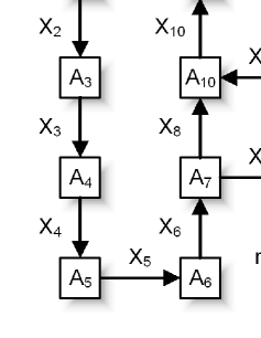
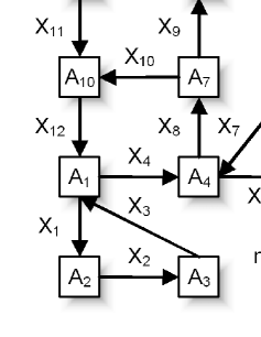
(a)	(b)	(c)

Figure 13: Illustrations of three irrigation network topologies: a. 6-ring, b. 6-ring-of-rings, and c. $3\times 3$ grid. Irrigation channels and their regulation devices are represented by arrows and rectangles. Inflow and outflow nodes are colored in light and dark gray. The ring and ring-of-rings networks are parameterized by the total number of regulation devices except for the last four ($n$).

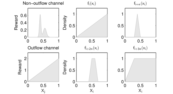
(a)	(b)                                  (c)

Figure 14: a. Indexing used in the description of the transition function in Example 6. The parameters $h$, $i$, $j$, and $k$ are equal to 6, 7, 10, and 1, respectively. b. Univariate reward functions over water levels $X_{j}$ (Example 6). c. Univariate basis functions over water levels $X_{i}$.

Similarly to Equation 45, we derive a utopian upper bound on the performance of any policy $\pi$ in an arbitrary irrigation network as:

$$\mathrm{E}_{\pi}\!\left[\sum_{t=0}^{\infty}\gamma^{t}R({\bf x}_{t},\pi({\bf x}_{t}))\right]\ \leq \ \ \frac{1}{1-\gamma}\Bigg{[}0.2n_{\mathrm{in}}+(n-n_{\mathrm{out}})$$

$$\ \ \max_{x}\int_{x^{\prime}}P_{\mathrm{beta}}(x^{\prime}\mid 46x+2,46(1-x)+2)R(x^{\prime})\,\mathrm{d}x^{\prime}\Bigg{]},$$ (46)

where $n$ is the total number of irrigation channels, $n_{\mathrm{in}}$ and $n_{\mathrm{out}}$ denote the number of inflow and outflow channels, respectively, and $R(x^{\prime})\!=\!\mathcal{N}(x^{\prime}\!\mid 0.4,0.025)/25.6+\mathcal{N}(x^{\prime}\!\mid 0.55,0.05)/32$. We do not analyze the quality of HALP solutions with respect to the optimal value function $V^{\ast}$ (Section 5.1) because this one is unknown.

Ring		$n=6$			$n=12$			$n=18$
topology		OV	Reward	Time	OV	Reward	Time	OV	Reward	Time
$\varepsilon$-HALP	$1/4$	$24.3$	$34.6\pm 2.0$	$11$	$36.2$	$53.9\pm 2.7$	$44$	$48.0$	$74.3\pm 2.9$	$87$
$\quad\varepsilon=$	$1/8$	$55.4$	$39.6\pm 2.5$	$41$	$88.1$	$61.5\pm 3.5$	$107$	$118.8$	$84.3\pm 3.8$	$178$
	$1/16$	$59.1$	$40.3\pm 2.6$	$281$	$93.2$	$62.6\pm 3.4$	$665$	$126.1$	$86.3\pm 3.8$	$1\ 119$
MCMC	$10$	$60.9$	$30.3\pm 4.9$	$38$	$86.3$	$47.6\pm 6.3$	$62$	$109.5$	$56.8\pm 7.4$	$87$
$\quad N=$	$50$	$70.1$	$40.2\pm 2.6$	$194$	$110.3$	$62.4\pm 3.5$	$328$	$148.8$	$85.0\pm 3.6$	$483$
	$250$	$70.7$	$40.2\pm 2.6$	$940$	$112.0$	$63.0\pm 3.4$	$1\ 609$	$151.7$	$85.4\pm 3.8$	$2\ 280$
MC	$10^{2}$	$16.2$	$25.0\pm 5.1$	$<1$	$16.9$	$41.9\pm 5.6$	$<1$	$17.2$	$51.8\pm 8.8$	$<1$
$\quad N=$	$10^{4}$	$40.8$	$37.9\pm 2.8$	$10$	$52.8$	$58.8\pm 3.5$	$18$	$63.8$	$75.9\pm 6.6$	$31$
	$10^{6}$	$51.2$	$39.4\pm 2.7$	$855$	$67.1$	$60.3\pm 3.8$	$1\ 415$	$81.1$	$82.9\pm 3.8$	$1\ 938$
Utopian			$49.1\qquad\>\;$			$79.2\qquad\>\;$			$109.2\qquad\>\;$
Ring-of-rings		$n=6$			$n=12$			$n=18$
topology		OV	Reward	Time	OV	Reward	Time	OV	Reward	Time
$\varepsilon$-HALP	$1/4$	$28.4$	$40.4\pm 2.5$	$85$	$44.1$	$66.5\pm 3.2$	$382$	$59.8$	$93.0\pm 3.8$	$931$
$\quad\varepsilon=$	$1/8$	$65.4$	$47.5\pm 3.0$	$495$	$107.9$	$76.1\pm 4.1$	$2\ 379$	$148.8$	$105.3\pm 4.2$	$5\ 877$
	$1/16$	$68.9$	$47.0\pm 2.9$	$4\ 417$	$113.1$	$77.3\pm 4.2$	$19\ 794$	$156.9$	$107.8\pm 4.1$	$53\ 655$
MCMC	$10$	$66.9$	$35.3\pm 6.1$	$60$	$94.6$	$54.4\pm 9.4$	$107$	$110.6$	$47.8\pm 13.2$	$157$
$\quad N=$	$50$	$80.9$	$47.1\pm 2.9$	$309$	$131.9$	$76.6\pm 3.6$	$571$	$181.4$	$104.6\pm 4.4$	$859$
	$250$	$81.7$	$47.2\pm 2.9$	$1\ 522$	$134.1$	$77.3\pm 3.5$	$2\ 800$	$186.0$	$106.6\pm 3.9$	$4\ 291$
MC	$10^{2}$	$13.7$	$31.0\pm 4.9$	$<1$	$15.4$	$46.1\pm 6.4$	$<1$	$16.8$	$66.6\pm 9.4$	$1$
$\quad N=$	$10^{4}$	$44.3$	$43.3\pm 3.2$	$12$	$59.0$	$68.9\pm 5.4$	$26$	$71.5$	$92.2\pm 6.8$	$49$
	$10^{6}$	$55.8$	$45.1\pm 3.1$	$1\ 026$	$75.1$	$74.3\pm 3.8$	$1\ 738$	$92.0$	$103.1\pm 4.2$	$2\ 539$
Utopian			$59.1\qquad\>\;$			$99.2\qquad\>\;$			$139.3\qquad\>\;$

Figure 15: Comparison of three HALP solvers on two irrigation network topologies of varying sizes ($n$). The solvers are compared by the objective value of a relaxed HALP (OV), the expected discounted reward of a corresponding policy, and computation time (in seconds). The $\varepsilon$-HALP, MCMC-HALP, and MC-HALP solvers are parameterized by the resolution of $\varepsilon$-grid ($\varepsilon$), the number of MCMC chains ($N$), and the number of samples ($N$). Note that the quality of policies improves with higher grid resolution ($1/\varepsilon$) and larger sample size ($N$). Upper bounds on their expected returns are shown in the last rows of the tables.

      Ring topology
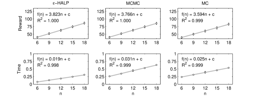
         Ring-of-rings topology

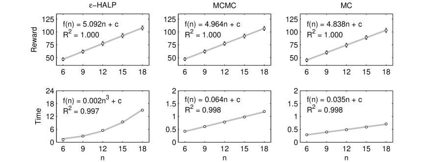
Figure 16: Scale-up potential of the $\varepsilon$-HALP, MCMC-HALP, and MC-HALP solvers on two irrigation network topologies of varying sizes ($n$). The graphs show the expected discounted reward of policies and their computation time (in hours) as functions of $n$. The HALP solvers are parameterized by the resolution of $\varepsilon$-grid ($\varepsilon=1/16$), the number of MCMC chains ($N=250$), and the number of samples ($N=10^{6}$). Note that all trends can be approximated by a polynomial $f(n)$ (gray line) with a high degree of confidence (the coefficient of determination $R^{2}$), where $c$ denotes a constant independent of $n$.

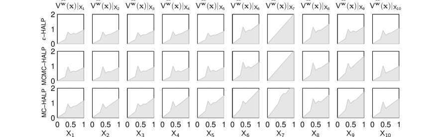
Figure 17: Univariate projections $V^{\widehat{{\bf w}}}({\bf x})|_{X_{j}}\!=\sum_{i:X_{j}=X_{i}}\widehat{w}_{i}f_{i}(x_{i})$ of approximate value functions $V^{\widehat{{\bf w}}}$ on the 6-ring irrigation network problem (Figure 13a). These functions are learned from 40 basis functions (Figure 14c) by the $\varepsilon$-HALP, MCMC-HALP, and MC-HALP solvers. The solvers are parameterized by the resolution of $\varepsilon$-grid ($\varepsilon=1/16$), the number of MCMC chains ($N=250$), and the number of samples ($N=10^{6}$). Note that the univariate projections $V^{\widehat{{\bf w}}}({\bf x})|_{X_{j}}$ are very similar. The proximity of their greedy policies can be explained based on this observation.

In the rest of the section, we illustrate the performance of three HALP approximations, MC-HALP, $\varepsilon$-HALP, and MCMC-HALP (Section 6), on the ring and ring-of-rings topologies (Figure 13) of the irrigation network problem. The constraints in the MC-HALP formulation are sampled uniformly at random. This establishes a baseline for all HALP approximations. The $\varepsilon$-HALP and MCMC-HALP formulations are generated iteratively by the cutting plane method. The MCMC oracle $\mathcal{O}_{\mathrm{MCMC}}$ is simulated for 500 steps from the initial temperature $c=0.2$, which leads to a decreasing cooling schedule from $T_{0}=0.2$ to $T_{500}\approx 0.02$. These parameters are selected empirically to demonstrate the characteristics of the oracle $\mathcal{O}_{\mathrm{MCMC}}$ rather than to maximize its performance. The value function $V^{\ast}$ is approximated by a linear combination of four univariate piecewise linear basis functions for each channel (Figure 14c). We assume that our basis functions are sufficient to derive a one-step lookahead policy that routes water between the channels if their water levels are too high or too low (Figure 14b). We believe that such a policy is close-to-optimal in irrigation networks. The state relevance density function $\psi({\bf x})$ is uniform. Our experimental results are reported in Figures 15–17.

Based on the results, we draw the following conclusions. First, all HALP approximations scale up in the dimensionality of solved problems. As shown in Figure 16, the return of the policies grows linearly in $n$. Moreover, the time complexity of computing them is polynomial in $n$. Therefore, if a problem and its approximate solution are structured, we take advantage of this structure to avoid an exponential blowup in the computation time. At the same time, the quality of the policies is not deteriorating with increasing problem size $n$.

Second, the MCMC solver ($N=250$) achieves the highest objective values on all solved problems. Higher objective values are interpreted as closer approximations to the constraint space in HALP since the solvers operate on relaxed formulations of HALP. Third, the quality of the MCMC-HALP policies ($N=250$) surpasses the MC-HALP policies ($N=10^{6}$) while both solvers consume approximately the same computation time. This result is due to the informative search for violated constraints in the MCMC-HALP solver. Fourth, the quality of the MCMC-HALP policies ($N=250$) is close to the $\varepsilon$-HALP policies ($\varepsilon=1/16$) although there is a significant difference between their objective values. Further analysis shows that the shape of the value functions is similar (Figure 17) and they differ the most in the weight of the constant basis function $f_{0}({\bf x})\equiv 1$. Note that increasing $w_{0}$ does not affect the quality of a greedy policy for $V^{\bf w}$. However, this trick allows the satisfaction of the constraint space in HALP (Section 5.1).

Finally, the computation time of the $\varepsilon$-HALP solver is seriously affected by the topologies of the irrigation networks, which can be explained as follows. For a small $\varepsilon$ and large $n$, the time complexity of formulating cost networks for the ring and ring-of-rings topologies grows by the rates of $\left\lceil 1/\varepsilon+1\right\rceil^{2}$ and $\left\lceil 1/\varepsilon+1\right\rceil^{3}$, respectively. Since the $\varepsilon$-HALP method consumes a significant amount of time by constructing cost networks, its quadratic (in $\left\lceil 1/\varepsilon+1\right\rceil$) time complexity on the ring topology worsens to cubic (in $\left\lceil 1/\varepsilon+1\right\rceil$) on the ring-of-rings topology. On the other hand, a similar cross-topology comparison of the MCMC-HALP solver shows that its computation times differ only by a multiplicative factor of 2. This difference is due to the increased complexity of sampling $p(z_{i}^{\ast}\mid{\bf z}_{-i})$, which results from more complex local dependencies in the ring-of-rings topology and not its treewidth.

Before we proceed, note that our relaxed formulations (Figure 15) have significantly less constraints than their complete sets (Section 6.3). For instance, the MC-HALP formulation ($N=10^{6}$) on the 6-ring irrigation network problem is originally established by $10^{6}$ randomly sampled constraints. Based on our empirical results, the constraints can be satisfied greedily by a subset of 400 constraints on average (?). Similarly, the oracle $\mathcal{O}_{\mathrm{MCMC}}$ in the MCMC-HALP formulation ($N=250$) iterates through $250\times 500\times(10+10)=2,500,000$ state-action configurations (Figure 11). However, corresponding LP formulations involve only 700 constraints on average.

7.3 The Curse of Treewidth

$\varepsilon$-HALP
$\varepsilon$	OV	Reward	Time
$1$	$30.4$	$48.3\pm 3.0$	$9$
$1/2$	$42.9$	$58.7\pm 3.1$	$342$
$1/4$	$49.1$	$61.9\pm 3.1$	$9\ 443$

MCMC
$N$	OV	Reward	Time
$10$	$45.3$	$43.6\pm 6.5$	$83$
$50$	$116.2$	$72.2\pm 3.6$	$458$
$250$	$118.5$	$73.2\pm 3.7$	$2\ 012$

MC
$N$	OV	Reward	Time
$10^{2}$	$12.8$	$56.6\pm 4.5$	$<1$
$10^{4}$	$49.9$	$53.4\pm 5.9$	$19$
$10^{6}$	$71.7$	$70.3\pm 3.9$	$1\ 400$

Figure 18: Comparison of three HALP solvers on the $3\times 3$ grid irrigation network problem (Figure 13). The solvers are compared by the objective value of a relaxed HALP (OV), the expected discounted reward of a corresponding policy, and computation time (in seconds). The $\varepsilon$-HALP, MCMC-HALP, and MC-HALP solvers are parameterized by the resolution of $\varepsilon$-grid ($\varepsilon$), the number of MCMC chains ($N$), and the number of samples ($N$). Note that the quality of policies improves with higher grid resolution ($1/\varepsilon$) and larger sample size ($N$). An upper bound on the expected returns is 87.2.

In the ring and ring-of-rings topologies, the treewidth of the constraint space (in continuous variables) is 2 and 3, respectively. As a result, the oracle $\mathcal{O}_{\varepsilon}$ can perform variable elimination for a small $\varepsilon$, and the $\varepsilon$-HALP solver returns close-to-optimal policies. Unfortunately, small treewidth is atypical in real-world domains. For instance, the treewidth of a more complex $3\times 3$ grid irrigation network (Figure 13c) is 6. To perform variable elimination for $\varepsilon=1/16$, the separation oracle $\mathcal{O}_{\varepsilon}$ requires the space of $\left\lceil 1/\varepsilon+1\right\rceil^{7}\!\approx\!2^{28}$, which is at the memory limit of existing PCs. To analyze the behavior of our separation oracles (Section 6) in this setting, we repeat our experiments from Section 7.2 on the $3\times 3$ grid irrigation network.

Based on the results in Figure 18, we conclude that the time complexity of the $\varepsilon$-HALP solver grows by the rate of $\left\lceil 1/\varepsilon+1\right\rceil^{7}$. Therefore, approximate constraint space satisfaction (MC-HALP and MCMC-HALP) generates better results than a combinatorial optimization on an insufficiently discretized $\varepsilon$-grid ($\varepsilon$-HALP). This conclusion is parallel to those in large structured optimization problems with continuous variables. We believe that a combination of exact and approximate steps delivers the best tradeoff between the quality and complexity of our solutions (Section 6.4).

8 Conclusions

Development of scalable algorithms for solving real-world decision problems is a challenging task. In this paper, we presented a theoretically sound framework that allows for a compact representation and efficient solutions to hybrid factored MDPs. We believe that our results can be applied to a variety of optimization problems in robotics, manufacturing, or financial mathematics. This work can be extended in several interesting directions.

First, note that the concept of closed-form solutions to the expectations terms in HALP is not limited to the choices in Section 5.2. For instance, we can show that if $P(x)$ and $f(x)$ are normal densities, $\mathrm{E}_{P(x)}\!\left[f(x)\right]$ has a closed-form solution (?). Therefore, we can directly reason with normal transition functions instead of approximating them by a mixture of beta distributions. Similar conclusions are true for piecewise constant, piecewise linear, and gamma transition and basis functions. Note that our efficient solutions apply to any approach to solving hybrid factored MDPs that approximates the optimal value function by a linear combination of basis functions (Equation 5).

Second, the constraint space in HALP (16) $V^{\bf w}-\mathcal{T}^{\ast}V^{\bf w}\geq 0$ exhibits the same structure as the constraint space in approximate policy iteration (API) (?, ?) $\left\|V^{\bf w}-\mathcal{T}^{\ast}V^{\bf w}\right\|_{\infty}\leq\varepsilon$, where $\varepsilon$ is a variable subject to minimization. As a result, our work provides a recipe for solving API formulations in hybrid state and action domains. In discrete-state spaces, ? (?) and ? (?) showed that API returns better policies than ALP for the same set of basis functions. Note that API is more complex than ALP because every step of API involves satisfying the constraint $\left\|V^{\bf w}-\mathcal{T}^{\ast}V^{\bf w}\right\|_{\infty}\leq\varepsilon$ for some fixed $\varepsilon$.

Third, automatic learning of basis functions seems critical for the application of HALP to real-world domains. ? (?) analyzed this problem in discrete-state spaces and proposed a greedy approach to learning basis functions. ? (?) generalized these ideas and showed how to learn parametric basis functions in hybrid spaces. We believe that a combination of the greedy search with a state space analysis (?, ?) can yield even better basis functions.

Finally, we proposed several bounds (Section 5.1 and 6.2.1) that may explain the quality of the complete and relaxed HALP formulations. In future, we plan to empirically evaluate their tightness on a variety of low-dimensional hybrid optimization problems (?, ?) with known optimal value functions.

A Proofs

Proof of Proposition 1: The Bellman operator $\mathcal{T}^{\ast}$ is known to be a contraction mapping. Based on its monotonicity, for any value function $V$, $V\geq\mathcal{T}^{\ast}V$ implies $V\geq\mathcal{T}^{\ast}V\geq\dots\geq V^{\ast}$. Since constraints in the HALP formulation (16) enforce $V^{\widetilde{{\bf w}}}\geq\mathcal{T}^{\ast}V^{\widetilde{{\bf w}}}$, we conclude $V^{\widetilde{{\bf w}}}\geq V^{\ast}$. $\square$

Proof of Proposition 2: Based on Proposition 1, we note that the constraint $V^{\bf w}\geq\mathcal{T}^{\ast}V^{\bf w}$ guarantees that $V^{\bf w}\geq V^{\ast}$. Subsequently, our claim is proved by realizing:

$$\arg\min_{\bf w}\mathrm{E}_{\psi}\!\left[V^{\bf w}\right]=\arg\min_{\bf w}\mathrm{E}_{\psi}\!\left[V^{\bf w}-V^{\ast}\right]$$

and

$$\mathrm{E}_{\psi}\!\left[V^{\bf w}-V^{\ast}\right]\ =\ \mathrm{E}_{\psi}\!\left|V^{\bf w}-V^{\ast}\right|$$

$$=\ \mathrm{E}_{\psi}\!\left|V^{\ast}-V^{\bf w}\right|$$

$$=\ \left\|V^{\ast}-V^{\bf w}\right\|_{1,\psi}.$$

The proof generalizes from the discrete-state case (?) without any alternations. $\square$

Proof of Theorem 2: Similarly to Theorem 2 (?), this claim is proved in three steps. First, we find a point $\overline{{\bf w}}$ in the feasible region of the HALP such that $V^{\overline{{\bf w}}}$ is within $O(\epsilon)$ distance from $V^{{\bf w}^{\ast}}$, where:

$${\bf w}^{\ast}\ =\ \arg\min_{\bf w}\left\|V^{\ast}-V^{\bf w}\right\|_{\infty}$$

$$\epsilon\ =\ \left\|V^{\ast}-V^{{\bf w}^{\ast}}\right\|_{\infty}.$$

Such a point $\overline{{\bf w}}$ is given by:

$$\overline{{\bf w}}={\bf w}^{\ast}+\frac{(1+\gamma)\epsilon}{1-\gamma}e,$$

where $e=(1,0,\dots,0)$ is an indicator of the constant basis function $f_{0}({\bf x})\equiv 1$. This point satisfies all requirements and its feasibility can be handily verified by solving:

$$V^{\overline{{\bf w}}}-\mathcal{T}^{\ast}V^{\overline{{\bf w}}}\ =\ V^{{\bf w}^{\ast}}+\frac{(1+\gamma)\epsilon}{1-\gamma}-\left(\mathcal{T}^{\ast}V^{{\bf w}^{\ast}}+\frac{\gamma(1+\gamma)\epsilon}{1-\gamma}\right)$$

$$=\ V^{{\bf w}^{\ast}}-\mathcal{T}^{\ast}V^{{\bf w}^{\ast}}+(1+\gamma)\epsilon$$

$$\geq\ 0,$$

where the last step follows from the inequality:

$$\left\|V^{{\bf w}^{\ast}}-\mathcal{T}^{\ast}V^{{\bf w}^{\ast}}\right\|_{\infty}\ \leq\ \left\|V^{{\bf w}^{\ast}}-V^{\ast}\right\|_{\infty}+\left\|V^{\ast}-\mathcal{T}^{\ast}V^{{\bf w}^{\ast}}\right\|_{\infty}$$

$$=\ \left\|V^{\ast}-V^{{\bf w}^{\ast}}\right\|_{\infty}+\left\|\mathcal{T}^{\ast}V^{\ast}-\mathcal{T}^{\ast}V^{{\bf w}^{\ast}}\right\|_{\infty}$$

$$\leq\ (1+\gamma)\epsilon.$$

Subsequently, we bound the max-norm error of $V^{\overline{{\bf w}}}$ by using the triangle inequality:

$$\left\|V^{\ast}-V^{\overline{{\bf w}}}\right\|_{\infty}\ \leq\ \left\|V^{\ast}-V^{{\bf w}^{\ast}}\right\|_{\infty}+\left\|V^{{\bf w}^{\ast}}-V^{\overline{{\bf w}}}\right\|_{\infty}$$

$$=\ \left(1+\frac{1+\gamma}{1-\gamma}\right)\epsilon$$

$$=\ \frac{2\epsilon}{1-\gamma},$$

which yields a bound on the weighted $\mathcal{L}_{1}$-norm error of $V^{\widetilde{{\bf w}}}$:

$$\left\|V^{\ast}-V^{\widetilde{{\bf w}}}\right\|_{1,\psi}\ \leq\ \left\|V^{\ast}-V^{\overline{{\bf w}}}\right\|_{1,\psi}$$

$$\leq\ \left\|V^{\ast}-V^{\overline{{\bf w}}}\right\|_{\infty}$$

$$\leq\ \frac{2\epsilon}{1-\gamma}.$$

The proof generalizes from the discrete-state case (?) without any alternations. $\square$

Proof of Theorem 3: Similarly to Theorem 2, this claim is proved in three steps: finding a point $\overline{{\bf w}}$ in the feasible region of the HALP, bounding the max-norm error of $V^{\overline{{\bf w}}}$, which in turn yields a bound on the $\mathcal{L}_{1}$-norm error of $V^{\widetilde{{\bf w}}}$. A comprehensive proof for the discrete-state case was done by ? (?). This proof generalizes to structured state and action spaces with continuous variables. $\square$

Proof of Proposition 3: The proposition is proved in a sequence of steps:

$$\mathrm{E}_{P(x)}\!\left[f(x)\right]\ =\ \int_{x}P_{\mathrm{beta}}(x\mid\alpha,\beta)x^{n}(1-x)^{m}\,\mathrm{d}x$$

$$=\ \int_{x}\frac{\Gamma(\alpha+\beta)}{\Gamma(\alpha)\Gamma(\beta)}x^{\alpha-1}(1-x)^{\beta-1}x^{n}(1-x)^{m}\,\mathrm{d}x$$

$$=\ \frac{\Gamma(\alpha+\beta)}{\Gamma(\alpha)\Gamma(\beta)}\int_{x}x^{\alpha+n-1}(1-x)^{\beta+m-1}\,\mathrm{d}x$$

$$=\ \frac{\Gamma(\alpha+\beta)}{\Gamma(\alpha)\Gamma(\beta)}\frac{\Gamma(\alpha+n)\Gamma(\beta+m)}{\Gamma(\alpha+\beta+n+m)}\int_{x}\frac{\Gamma(\alpha+\beta+n+m)}{\Gamma(\alpha+n)\Gamma(\beta+m)}x^{\alpha+n-1}(1-x)^{\beta+m-1}\,\mathrm{d}x$$

$$=\ \frac{\Gamma(\alpha+\beta)}{\Gamma(\alpha)\Gamma(\beta)}\frac{\Gamma(\alpha+n)\Gamma(\beta+m)}{\Gamma(\alpha+\beta+n+m)}\underbrace{\int_{x}P_{\mathrm{beta}}(x\mid\alpha+n,\beta+m)\,\mathrm{d}x}_{1}.$$

Since integration is a distributive operation, our claim straightforwardly generalizes to the mixture of beta distributions $P(x)$. $\square$

Proof of Proposition 4: The proposition is proved in a sequence of steps:

$$\mathrm{E}_{P(x)}\!\left[f(x)\right]\ =\ \int_{x}P_{\mathrm{beta}}(x\mid\alpha,\beta)\sum_{i}\mathbf{1}_{[l_{i},r_{i}]}(x)(a_{i}x+b_{i})\,\mathrm{d}x$$

$$=\ \sum_{i}\int_{l_{i}}^{r_{i}}P_{\mathrm{beta}}(x\mid\alpha,\beta)(a_{i}x+b_{i})\,\mathrm{d}x$$

$$=\ \sum_{i}\left[a_{i}\int_{l_{i}}^{r_{i}}P_{\mathrm{beta}}(x\mid\alpha,\beta)x\,\mathrm{d}x+b_{i}\int_{l_{i}}^{r_{i}}P_{\mathrm{beta}}(x\mid\alpha,\beta)\,\mathrm{d}x\right]$$

$$=\ \sum_{i}\left[a_{i}\frac{\alpha}{\alpha+\beta}\int_{l_{i}}^{r_{i}}P_{\mathrm{beta}}(x\mid\alpha+1,\beta)\,\mathrm{d}x+b_{i}\int_{l_{i}}^{r_{i}}P_{\mathrm{beta}}(x\mid\alpha,\beta)\,\mathrm{d}x\right]$$

$$=\ \sum_{i}\left[a_{i}\frac{\alpha}{\alpha+\beta}(F^{+}(r_{i})-F^{+}(l_{i}))+b_{i}(F(r_{i})-F(l_{i}))\right].$$

Since integration is a distributive operation, our claim straightforwardly generalizes to the mixture of beta distributions $P(x)$. $\square$

Proof of Proposition 5: This claim is proved in three steps. First, we construct a point $\overline{{\bf w}}$ in the feasible region of the HALP such that $V^{\overline{{\bf w}}}$ is within $O(\delta)$ distance from $V^{\widehat{{\bf w}}}$. Such a point $\overline{{\bf w}}$ is given by:

$$\overline{{\bf w}}=\widehat{{\bf w}}+\frac{\delta}{1-\gamma}e,$$

where $e=(1,0,\dots,0)$ is an indicator of the constant basis function $f_{0}({\bf x})\equiv 1$. This point satisfies all requirements and its feasibility can be handily verified by solving:

$$V^{\overline{{\bf w}}}-\mathcal{T}^{\ast}V^{\overline{{\bf w}}}\ =\ V^{\widehat{{\bf w}}}+\frac{\delta}{1-\gamma}-\left(\mathcal{T}^{\ast}V^{\widehat{{\bf w}}}+\frac{\gamma\delta}{1-\gamma}\right)$$

$$=\ V^{\widehat{{\bf w}}}-\mathcal{T}^{\ast}V^{\widehat{{\bf w}}}+\delta$$

$$\geq\ 0,$$

where the inequality $V^{\widehat{{\bf w}}}-\mathcal{T}^{\ast}V^{\widehat{{\bf w}}}\geq-\delta$ holds from the $\delta$-infeasibility of $\widehat{{\bf w}}$. Since the optimal solution $\widetilde{{\bf w}}$ is feasible in the relaxed HALP, we conclude $\mathrm{E}_{\psi}\!\left[V^{\widehat{{\bf w}}}\right]\leq\mathrm{E}_{\psi}\!\left[V^{\widetilde{{\bf w}}}\right]$. Subsequently, this inequality yields a bound on the weighted $\mathcal{L}_{1}$-norm error of $V^{\overline{{\bf w}}}$:

$$\left\|V^{\ast}-V^{\overline{{\bf w}}}\right\|_{1,\psi}\ =\ \mathrm{E}_{\psi}\!\left|V^{\widehat{{\bf w}}}+\frac{\delta}{1-\gamma}-V^{\ast}\right|$$

$$=\ \mathrm{E}_{\psi}\!\left[V^{\widehat{{\bf w}}}\right]+\frac{\delta}{1-\gamma}-\mathrm{E}_{\psi}\!\left[V^{\ast}\right]$$

$$\leq\ \mathrm{E}_{\psi}\!\left[V^{\widetilde{{\bf w}}}\right]+\frac{\delta}{1-\gamma}-\mathrm{E}_{\psi}\!\left[V^{\ast}\right]$$

$$=\ \left\|V^{\ast}-V^{\widetilde{{\bf w}}}\right\|_{1,\psi}+\frac{\delta}{1-\gamma}.$$

Finally, we combine this result with the triangle inequality:

$$\left\|V^{\ast}-V^{\widehat{{\bf w}}}\right\|_{1,\psi}\ \leq\ \left\|V^{\ast}-V^{\overline{{\bf w}}}\right\|_{1,\psi}+\left\|V^{\overline{{\bf w}}}-V^{\widehat{{\bf w}}}\right\|_{1,\psi}$$

$$\leq\ \left\|V^{\ast}-V^{\widetilde{{\bf w}}}\right\|_{1,\psi}+\frac{2\delta}{1-\gamma},$$

which leads to a bound on the weighted $\mathcal{L}_{1}$-norm error of $V^{\widehat{{\bf w}}}$. $\square$

References

- Andrieu et al. Andrieu, C., de Freitas, N., Doucet, A., and Jordan, M. (2003). An introduction to MCMC for machine learning. Machine Learning, 50, 5–43.
- Astrom Astrom, K. (1965). Optimal control of Markov processes with incomplete state information. Journal of Mathematical Analysis and Applications, 10(1), 174–205.
- Bellman Bellman, R. (1957). Dynamic Programming. Princeton University Press, Princeton, NJ.
- Bellman et al. Bellman, R., Kalaba, R., and Kotkin, B. (1963). Polynomial approximation – a new computational technique in dynamic programming: Allocation processes. Mathematics of Computation, 17(82), 155–161.
- Bertsekas Bertsekas, D. (1995). A counterexample for temporal differences learning. Neural Computation, 7(2), 270–279.
- Bertsekas and Tsitsiklis Bertsekas, D., and Tsitsiklis, J. (1996). Neuro-Dynamic Programming. Athena Scientific, Belmont, MA.
- Bertsimas and Tsitsiklis Bertsimas, D., and Tsitsiklis, J. (1997). Introduction to Linear Optimization. Athena Scientific, Belmont, MA.
- Boutilier et al. Boutilier, C., Dearden, R., and Goldszmidt, M. (1995). Exploiting structure in policy construction. In Proceedings of the 14th International Joint Conference on Artificial Intelligence, pp. 1104–1111.
- Bresina et al. Bresina, J., Dearden, R., Meuleau, N., Ramakrishnan, S., Smith, D., and Washington, R. (2002). Planning under continuous time and resource uncertainty: A challenge for AI. In Proceedings of the 18th Conference on Uncertainty in Artificial Intelligence, pp. 77–84.
- Casella and Robert Casella, G., and Robert, C. (1996). Rao-Blackwellisation of sampling schemes. Biometrika, 83(1), 81–94.
- Chow and Tsitsiklis Chow, C.-S., and Tsitsiklis, J. (1991). An optimal one-way multigrid algorithm for discrete-time stochastic control. IEEE Transactions on Automatic Control, 36(8), 898–914.
- Cooper Cooper, G. (1988). A method for using belief networks as influence diagrams. In Proceedings of the Workshop on Uncertainty in Artificial Intelligence, pp. 55–63.
- Crites and Barto Crites, R., and Barto, A. (1996). Improving elevator performance using reinforcement learning. In Advances in Neural Information Processing Systems 8, pp. 1017–1023.
- de Farias and Van Roy de Farias, D. P., and Van Roy, B. (2003). The linear programming approach to approximate dynamic programming. Operations Research, 51(6), 850–856.
- de Farias and Van Roy de Farias, D. P., and Van Roy, B. (2004). On constraint sampling for the linear programming approach to approximate dynamic programming. Mathematics of Operations Research, 29(3), 462–478.
- Dean and Kanazawa Dean, T., and Kanazawa, K. (1989). A model for reasoning about persistence and causation. Computational Intelligence, 5, 142–150.
- Dechter Dechter, R. (1996). Bucket elimination: A unifying framework for probabilistic inference. In Proceedings of the 12th Conference on Uncertainty in Artificial Intelligence, pp. 211–219.
- Duane et al. Duane, S., Kennedy, A. D., Pendleton, B., and Roweth, D. (1987). Hybrid Monte Carlo. Physics Letters B, 195(2), 216–222.
- Feng et al. Feng, Z., Dearden, R., Meuleau, N., and Washington, R. (2004). Dynamic programming for structured continuous Markov decision problems. In Proceedings of the 20th Conference on Uncertainty in Artificial Intelligence, pp. 154–161.
- Ferns et al. Ferns, N., Panangaden, P., and Precup, D. (2005). Metrics for Markov decision processes with infinite state spaces. In Proceedings of the 21st Conference on Uncertainty in Artificial Intelligence.
- Geman and Geman Geman, S., and Geman, D. (1984). Stochastic relaxation, Gibbs distribution, and the Bayesian restoration of images. IEEE Transactions on Pattern Analysis and Machine Intelligence, 6(6), 721–741.
- Gordon Gordon, G. (1999). Approximate Solutions to Markov Decision Processes. Ph.D. thesis, Carnegie Mellon University.
- Guestrin Guestrin, C. (2003). Planning Under Uncertainty in Complex Structured Environments. Ph.D. thesis, Stanford University.
- Guestrin et al. Guestrin, C., Hauskrecht, M., and Kveton, B. (2004). Solving factored MDPs with continuous and discrete variables. In Proceedings of the 20th Conference on Uncertainty in Artificial Intelligence, pp. 235–242.
- Guestrin et al. Guestrin, C., Koller, D., Gearhart, C., and Kanodia, N. (2003). Generalizing plans to new environments in relational MDPs. In Proceedings of the 18th International Joint Conference on Artificial Intelligence, pp. 1003–1010.
- Guestrin et al. Guestrin, C., Koller, D., and Parr, R. (2001). Max-norm projections for factored MDPs. In Proceedings of the 17th International Joint Conference on Artificial Intelligence, pp. 673–682.
- Guestrin et al. Guestrin, C., Koller, D., and Parr, R. (2002). Multiagent planning with factored MDPs. In Advances in Neural Information Processing Systems 14, pp. 1523–1530.
- Guestrin et al. Guestrin, C., Koller, D., Parr, R., and Venkataraman, S. (2003). Efficient solution algorithms for factored MDPs. Journal of Artificial Intelligence Research, 19, 399–468.
- Guestrin et al. Guestrin, C., Venkataraman, S., and Koller, D. (2002). Context specific multiagent coordination and planning with factored MDPs. In Proceedings of the 18th National Conference on Artificial Intelligence, pp. 253–259.
- Hastings Hastings, W. K. (1970). Monte Carlo sampling methods using Markov chains and their application. Biometrika, 57, 97–109.
- Hauskrecht Hauskrecht, M. (2000). Value-function approximations for partially observable Markov decision processes. Journal of Artificial Intelligence Research, 13, 33–94.
- Hauskrecht and Kveton Hauskrecht, M., and Kveton, B. (2004). Linear program approximations for factored continuous-state Markov decision processes. In Advances in Neural Information Processing Systems 16, pp. 895–902.
- Higdon Higdon, D. (1998). Auxiliary variable methods for Markov chain Monte Carlo with applications. Journal of the American Statistical Association, 93(442), 585–595.
- Howard and Matheson Howard, R., and Matheson, J. (1984). Influence diagrams. In Readings on the Principles and Applications of Decision Analysis, Vol. 2, pp. 719–762. Strategic Decisions Group, Menlo Park, CA.
- Jeffreys and Jeffreys Jeffreys, H., and Jeffreys, B. (1988). Methods of Mathematical Physics. Cambridge University Press, Cambridge, United Kingdom.
- Jensen et al. Jensen, F., Jensen, F., and Dittmer, S. (1994). From influence diagrams to junction trees. In Proceedings of the 10th Conference on Uncertainty in Artificial Intelligence, pp. 367–373.
- Khachiyan Khachiyan, L. (1979). A polynomial algorithm in linear programming. Doklady Akademii Nauk SSSR, 244, 1093–1096.
- Kirkpatrick et al. Kirkpatrick, S., Gelatt, C. D., and Vecchi, M. P. (1983). Optimization by simulated annealing. Science, 220(4598), 671–680.
- Koller and Parr Koller, D., and Parr, R. (1999). Computing factored value functions for policies in structured MDPs. In Proceedings of the 16th International Joint Conference on Artificial Intelligence, pp. 1332–1339.
- Kveton and Hauskrecht Kveton, B., and Hauskrecht, M. (2004). Heuristic refinements of approximate linear programming for factored continuous-state Markov decision processes. In Proceedings of the 14th International Conference on Automated Planning and Scheduling, pp. 306–314.
- Kveton and Hauskrecht Kveton, B., and Hauskrecht, M. (2005). An MCMC approach to solving hybrid factored MDPs. In Proceedings of the 19th International Joint Conference on Artificial Intelligence, pp. 1346–1351.
- Kveton and Hauskrecht Kveton, B., and Hauskrecht, M. (2006a). Learning basis functions in hybrid domains. In Proceedings of the 21st National Conference on Artificial Intelligence, pp. 1161–1166.
- Kveton and Hauskrecht Kveton, B., and Hauskrecht, M. (2006b). Solving factored MDPs with exponential-family transition models. In Proceedings of the 16th International Conference on Automated Planning and Scheduling, pp. 114–120.
- Mahadevan Mahadevan, S. (2005). Samuel meets Amarel: Automating value function approximation using global state space analysis. In Proceedings of the 20th National Conference on Artificial Intelligence, pp. 1000–1005.
- Mahadevan and Maggioni Mahadevan, S., and Maggioni, M. (2006). Value function approximation with diffusion wavelets and Laplacian eigenfunctions. In Advances in Neural Information Processing Systems 18, pp. 843–850.
- Mahadevan et al. Mahadevan, S., Maggioni, M., Ferguson, K., and Osentoski, S. (2006). Learning representation and control in continuous Markov decision processes. In Proceedings of the 21st National Conference on Artificial Intelligence.
- Manne Manne, A. (1960). Linear programming and sequential decisions. Management Science, 6(3), 259–267.
- Metropolis et al. Metropolis, N., Rosenbluth, A., Rosenbluth, M., Teller, A., and Teller, E. (1953). Equation of state calculations by fast computing machines. Journal of Chemical Physics, 21, 1087–1092.
- Munos and Moore Munos, R., and Moore, A. (2002). Variable resolution discretization in optimal control. Machine Learning, 49, 291–323.
- Ortiz Ortiz, L. (2002). Selecting Approximately-Optimal Actions in Complex Structured Domains. Ph.D. thesis, Brown University.
- Park and Darwiche Park, J., and Darwiche, A. (2001). Approximating MAP using local search. In Proceedings of the 17th Conference on Uncertainty in Artificial Intelligence, pp. 403–410.
- Park and Darwiche Park, J., and Darwiche, A. (2003). Solving MAP exactly using systematic search. In Proceedings of the 19th Conference on Uncertainty in Artificial Intelligence, pp. 459–468.
- Patrascu et al. Patrascu, R., Poupart, P., Schuurmans, D., Boutilier, C., and Guestrin, C. (2002). Greedy linear value-approximation for factored Markov decision processes. In Proceedings of the 18th National Conference on Artificial Intelligence, pp. 285–291.
- Puterman Puterman, M. (1994). Markov Decision Processes: Discrete Stochastic Dynamic Programming. John Wiley & Sons, New York, NY.
- Rust Rust, J. (1997). Using randomization to break the curse of dimensionality. Econometrica, 65(3), 487–516.
- Sanner and Boutilier Sanner, S., and Boutilier, C. (2005). Approximate linear programming for first-order MDPs. In Proceedings of the 21st Conference on Uncertainty in Artificial Intelligence.
- Schuurmans and Patrascu Schuurmans, D., and Patrascu, R. (2002). Direct value-approximation for factored MDPs. In Advances in Neural Information Processing Systems 14, pp. 1579–1586.
- Schweitzer and Seidmann Schweitzer, P., and Seidmann, A. (1985). Generalized polynomial approximations in Markovian decision processes. Journal of Mathematical Analysis and Applications, 110, 568–582.
- Sondik Sondik, E. (1971). The Optimal Control of Partially Observable Markov Decision Processes. Ph.D. thesis, Stanford University.
- Sutton and Barto Sutton, R., and Barto, A. (1998). Reinforcement Learning: An Introduction. MIT Press, Cambridge, MA.
- Tesauro Tesauro, G. (1992). Practical issues in temporal difference learning. Machine Learning, 8(3-4), 257–277.
- Tesauro Tesauro, G. (1994). TD-Gammon, a self-teaching backgammon program, achieves master-level play. Neural Computation, 6(2), 215–219.
- Tesauro Tesauro, G. (1995). Temporal difference learning and TD-Gammon. Communications of the ACM, 38(3), 58–68.
- Trick and Zin Trick, M., and Zin, S. (1993). A linear programming approach to solving stochastic dynamic programs. Tech. rep., Carnegie Mellon University.
- Van Roy Van Roy, B. (1998). Planning Under Uncertainty in Complex Structured Environments. Ph.D. thesis, Massachusetts Institute of Technology.
- Yuan et al. Yuan, C., Lu, T.-C., and Druzdzel, M. (2004). Annealed MAP. In Proceedings of the 20th Conference on Uncertainty in Artificial Intelligence, pp. 628–635.
- Zhang and Dietterich Zhang, W., and Dietterich, T. (1995). A reinforcement learning approach to job-shop scheduling. In Proceedings of the 14th International Joint Conference on Artificial Intelligence, pp. 1114–1120.
- Zhang and Dietterich Zhang, W., and Dietterich, T. (1996). High-performance job-shop scheduling with a time-delay TD() network. In Advances in Neural Information Processing Systems 8, pp. 1024–1030.