Learning to relate images: Mapping units,
complex cells and simultaneous eigenspaces

Abstract

A fundamental operation in many vision tasks, including motion understanding, stereopsis, visual odometry, or invariant recognition, is establishing correspondences between images or between images and data from other modalities. We present an analysis of the role that multiplicative interactions play in learning such correspondences, and we show how learning and inferring relationships between images can be viewed as detecting rotations in the eigenspaces shared among a set of orthogonal matrices. We review a variety of recent multiplicative sparse coding methods in light of this observation. We also review how the squaring operation performed by energy models and by models of complex cells can be thought of as a way to implement multiplicative interactions. This suggests that the main utility of including complex cells in computational models of vision may be that they can encode relations not invariances.

1 Introduction

Correspondence is arguably the most ubiquitous computational primitive in vision: Tracking amounts to establishing correspondences between frames; stereo vision between different views of a scene; optical flow between any two images; invariant recognition between images and invariant descriptions in memory; odometry between images and motion information; action recognition between frames; etc. In these and many other tasks, the relationship between images not the content of a single image carries the relevant information. Representing structures within a single image, such as contours, can be also considered as an instance of a correspondence problem, namely between areas, or pixels, within an image. The fact that correspondence is such a common operation across vision suggests that the task of representing relations may have to be kept in mind when trying to build autonomous vision systems and when trying to understand biological vision.

A lot of progress has been made recently in building models that learn to solve tasks like object recognition from independent, static images. One of the reasons for the recent progress is the use of local features, which help virtually eliminate the notoriously difficult problems of occlusions and small invariances. A central finding is that the right choice of features not the choice of high-level classifier or computational pipeline are what typically makes a system work well. Interestingly, some of the best performing recognition models are highly biologically consistent, in that they are based on features that are learned unsupervised from data. Besides being biological plausible, feature learning comes with various benefits, such as helping overcome tedious engineering, helping adapt to new domains and allowing for some degree of end-to-end learning in place of constructing, and then combining, a large number of modules to solve a task. The fact that tasks like object recognition can be solved using biologically consistent, learning based methods raises the question whether understanding relations can be amenable to learning in the same way. If so, this may open up the road to learning based and/or biologically consistent approaches to a much larger variety of problems than static object recognition, and perhaps also beyond vision.

In this paper, we review a variety of recent methods that address correspondence tasks by learning local features. We discuss how the common computational principle behind all these methods are multiplicative interactions, which were introduced to the vision community $30$ years ago under the terms “mapping units” [18] and “dynamic mappings” [48]. An illustration of mapping units is shown in Figure 1: The three variables shown in the figure interact multiplicatively, and as a result, each variable (say, $z_{k}$) can be thought of as dynamically modulating the connections between other variables in the model ($x_{i}$ and $y_{j}$). Likewise, the value of any variable (eg., $y_{j}$) can be thought of as depending on the product of the other variables ($x_{i}$, $z_{k}$) [18]. This is in contrast to common feature learning models like ICA, Restricted Boltzmann Machines, auto-encoder networks and many others, all of which are based on bi-partite networks, that do not involve any three-way multiplicative interactions. In these models, independent hidden variables interact with independent observable variables, such that the value of any variable depends on a weighted sum not product of the other variables. Closely related to models of mapping units are energy models (for example, [1]), which may be thought of as a way to “emulate” multiplicative interactions by computing squares.

We shall show how both mapping units and energy models can be viewed as ways to learn and detect rotations in a set of shared invariant subspaces of a set of commuting matrices. Our analysis may help understand why action recognition methods seem to profit from squaring non-linearities (for example, [27]), and it predicts that squaring and cross-products will be helpful, in general, in applications that involve representing relations.

1.1 A brief history of multiplicative interactions

Shortly after mapping units were introduced in $1981$, energy models [1] received a lot of attention. Energy models are closely related to cross-correlation models [2], which, in turn, are a type of multiplicative interaction model. Energy models have been used as a way to model motion (relating time frames in a video) [1] and stereo vision (relating images across different eyes or cameras) [33]. An energy model is a computational unit that relates images by summing over squared responses of, typically two, linear projections of input data. This operation can be shown to encode translations independently of content [7], [37] (cf. Section 3).

Early approaches to building and applying energy and cross-correlation models were based entirely on hand-wiring (see, for example, [37], [41], [7]). Practically all of these models use Gabor filters as the linear receptive fields whose responses are squared and summed. The focus on Gabor features has somewhat biased the analysis of energy models to focus on the Fourier-spectrum as the main object of interest (see, for example, [7, 37]). As we shall discuss in Section 3, Fourier-components arise just as the special case of one transformation class, namely translation, and many of the analyses apply more generally and to other types of transformation.

Gabor-based energy models have also been applied monocularly. In this case they encode features independently of the Fourier-phase of the input. As a result, their responses are invariant to small translations as well as to contrast variations of the input. In part for this reason, energy models have been popular in models of complex cells, which are known to show similar invariance properties (see, for example, [22]).

Shortly after energy and cross-correlation models emerged, there has been some attention on learning invariances with higher-order neural networks, which are neural networks trained on polynomial basis expansions of their inputs, [11]. Higher-order neural networks can be composed of units that compute sums of products. These units are sometimes referred to as “Sigma-Pi-units” [40] (where “Pi” stands for product and “Sigma” for sum). [42], at about the same time, discussed how multiplicative interactions make it possible to build distributed representations of symbolic data.

Figure 1: Symbolic representation of a mapping unit [18]. The triangle symbolizes multiplicative interactions between the three variables $z_{k}$, $x_{i}$ and $y_{j}$. The value of any one of the three variables is a function of the product of all the others. ([18]).

In 1995, Kohonen introduced the “Adaptive Subspace Self-Organizing Map” (ASSOM) [26], which computes sums over squared filter responses to represent data. Like the energy model, the ASSOM is based on the idea that the sum of squared responses is invariant to various properties of its inputs. In contrast to the early energy models, the ASSOM is trained from data. Inspired by the ASSOM, [23] introduced “Independent Subspace Analysis” (ISA), which puts the same idea into the context of more conventional sparse coding models. Extensions of this work are topographic ICA [23] and [50], where sums are computed not over separate but over shared groups of squared filter responses.

In a parallel line of work, bi-linear models were used as an approach to learning in the presence of multiplicative interactions [45]. This early work on bi-linear models used these as global models trained on whole images rather than using local receptive fields. In contrast to more recent approaches to learning with multiplicative interactions, training typically involved filling a two-dimensional grid with data that shows two types of variability (sometimes called “style” and “content”). The purpose of bi-linear models is then to untangle the two degrees of freedom in the data. More recent work does not make this distinction, and the purpose of multiplicative hidden variables is merely to capture the multiple ways in which two images can be related. [13], [36], [30], for example, show how multiplicative interactions make it possible to model the multitude of relationships between frames in natural videos. [30] also show how they allow us to model more general classes of relations between images. An earlier multiplicative interaction model, that is also related to bi-linear models, is the “routing-circuit” [35].

Multiplicative interactions have also been used to model structure within static images, which can be thought of as modeling higher-order relations, and, in particular, pair-wise products, between pixel intensities (for example, [25, 23, 49, 21, 38, 6, 29]).

Recently, [32] showed how multiplicative interactions between a class-label and a feature vector can be viewed as an invariant classifier, where each class is represented by a manifold of allowable transformations. This work may be viewed as a modern version of the model that introduced the term mapping units in 1981 [18]. The main difference between 2011 and 1981 is that models are now trained from large datasets.

2 Learning to relate images

2.1 Feature learning

We briefly review standard feature learning models in this section and we discuss relational feature learning in Section 2.2. We discuss extensions of relational models and how they relate to complex cells and to energy models in Section 3.

Practically all standard feature learning models can be represented by a graphical model like the one shown in Figure 2 (a). The model is a bi-partite network that connects a set of unobserved, latent variables $z_{k}$ with a set of observable variables (for example, pixels) $y_{j}$. The weights $w_{jk}$, which connect pixel $y_{j}$ with hidden unit $z_{k}$, are learned from a set of training images $\{\bm{y}^{\alpha}\}_{\alpha=1,\ldots,N}$. The vector of latent variables $\bm{z}=(z_{k})_{k=1\ldots K}$ in Figure 2 (a) is considered to be unobserved, so one has to infer it, separately for each training case, along with the model parameters for training. The graphical model shown in the figure represents how the dependencies between components $y_{i}$ and $z_{k}$ are parameterized, but it does not define a model or learning algorithm. A large variety of models and learning algorithms can be parameterized as in the figure, including principal components, mixture models, k-means clustering, or restricted Boltzmann machines [16]. Each of these can in principle be used as a feature learning method (see, for example, [5] for a recent quantitative comparison).

For the hidden variables to extract useful structure from the images, their capacity needs to be constrained. The simplest form of constraining it is to let the dimensionality $K$ be smaller than the dimensionality $J$ of the images. Learning in this case amounts to performing dimensionality reduction. It has become obvious recently that it is more useful in most applications to use an over-complete representation, that is, $K>J$, and to constrain the capacity of the latent variables instead by forcing the hidden unit activities to be sparse. In Figure 2, and in what follows, we use $K<J$ to symbolize the fact that $\bm{z}$ is capacity-constrained, but it should be kept in mind that capacity can be (and often is) constrained in other ways. The most common operations in the model, after training, are: “Inference” (or “Analysis”): Given image $\bm{y}$, compute $\bm{z}$; and “Generation” (or “Synthesis”): Invent a latent vector $\bm{z}$, then compute $\bm{y}$.

(a)	(b)

Figure 2: (a) Sparse coding graphical model. (b) Auto-encoder network.

A simple way to train a model, given training images, is by minimizing reconstruction error combined with a sparsity encouraging term for the hidden variables (for example, [34]):

$$\sum_{\alpha}\big{(}\|\bm{y}^{\alpha}-\sum_{k}z_{k}^{\alpha}W_{.k}\|^{2}+\lambda|z_{k}^{\alpha}|\big{)}$$ (1)

Optimization is with respect to both $W=(w_{jk})_{j=1\ldots J,k=1\ldots K}$ and all $\bm{z}^{\alpha}$. For this end, it is common to alternate between optimizing $W$ and optimizing all $\bm{z}^{\alpha}$. After training, inference then amounts to minimizing the same expression for test images (with $W$ fixed).

To avoid iterative optimization during inference, one can eliminate $\bm{z}$ by defining it implicitly as a function of $\bm{y}$. A common choice of function is $\bm{z}=\sigma\left(A\bm{y}\right)$ where $A$ is a matrix and $\sigma(\cdot)$ is a squashing non-linearity, such as $\sigma(a)=(1+\exp(-a))^{-1}$, which confines the values of $\bm{z}$ to reside in a fixed interval. This model is the well-known auto-encoder (for example, [47]) and it is depicted in Figure 2. Learning amounts to minimizing reconstruction error with respect to both $A$ and $W$. In practice, it is common to enforce $A:=W^{\mathrm{T}}$ in order to reduce the number of parameters and for consistency with other sparse coding models.

One can add a penalty term that encourages sparsity of the latent variables. Alternatively, one can train auto-encoders, such that they de-noise corrupted version of their inputs, which can be achieved by simply feeding in corrupted inputs during training (but measuring reconstruction error with respect to the original data). This turns auto-encoders into “de-noising auto-encoders” [47], which show properties similar to other sparse coding methods, but inference, like in a standard auto-encoder, is a simple feed-forward mapping.

A technique similar to the auto-encoder is the Restricted Boltzmann machine (RBM): RBMs define the joint probability distribution

$$p(\bm{y},\bm{z})=\frac{1}{Z}\exp\big{(}\sum_{jk}w_{jk}y_{j}z_{k}\big{)},$$ (2)

from which one can derive

$$p(z_{k}|\bm{y})=\mathrm{sigmoid}\big{(}\sum_{j}w_{jk}y_{j}\big{)}\quad\mbox{and}\quad p(y_{j}|\bm{z})=\mathrm{sigmoid}\big{(}\sum_{j}w_{jk}z_{k}\big{)},$$ (3)

showing that inference, again, amounts to a linear mapping plus non-linearity. Learning amounts to maximizing the average log-probability $\frac{1}{N}\sum_{\alpha}\log p(\bm{y}^{\alpha})$ of the training data. Since the derivatives with respect to the parameters are not tractable (due to the normalizing constant $Z$ in Eq. 2), it is common to use approximate Gibbs sampling in order to approximate them. This leads to a Hebbian-like learning rule known as contrastive divergence training [16].

Another common sparse coding method is independent components analysis (ICA) (for example, [22]). One way to train an ICA-model that is complete (that is, where $\bm{z}$ has the same size as $\bm{y}$) is by encouraging latent responses to be sparse, while preventing weights from becoming degenerate [22]:

$$\min_{W}\|W^{\mathrm{T}}\bm{y}\|_{1}$$ (4)

$$\mathrm{s.t.}\quad W^{\mathrm{T}}W=I$$ (5)

Enforcing the constraint can be inefficient in practice, since it requires an eigen decomposition.

For most feature learning models, inference and generation are variations of the two linear mappings:

$$z_{k}=\sum_{j}w_{jk}y_{j}$$ (6)

$$y_{j}=\sum_{k}w_{jk}z_{k}$$ (7)

The set of model parameters $W_{\cdot k}$ for any $k$ are typically referred to as “features” or “filters” (although a more appropriate term would be “basis functions”; we shall use these interchangeably). Practically all methods yield Gabor-like features when trained on natural images. An advantage of non-linear models, such as RBM’s and auto-encoders, is that stacking them makes it possible to learn feature hierarchies (“deep learning”) [17].

In practice, it is common to add bias terms, such that inference and generation (Eqs. 6 and 7) are affine not linear functions, for example, $y_{j}=\sum_{k}w_{jk}z_{k}+b_{j}$ for some parameter $b_{j}$. We shall refrain from adding bias terms to avoid clutter, noting that, alternatively, one may think of $\bm{y}$ and $\bm{z}$ as being in “homogeneous” coordinates, containing an extra, constant $1$-dimension.

Feature learning is typically performed on small images patches of size between around $5\times 5$ and $50\times 50$ pixels. One reason for this is that training and inference can be computationally demanding. More important, local features make it possible to deal with images of different size, and to deal with occlusions and local object variations. Given a trained model, two common ways to perform invariant recognition on test images are:

“Bag-Of-Features”: Crop patches around interest points (such as SIFT or Harris corners), compute latent representation $\bm{z}$ for each patch, collapse (add up) all representations to obtain a single vector $\bm{z}^{\mathrm{Image}}$, classify $\bm{z}^{\mathrm{Image}}$ using a standard classifier. There are several variations of this scheme, including using an extra clustering-step before collapsing features, or using a histogram-similarity in place of Euclidean distance for the collapsed representation.

“Convolutional”: Crop patches from the image along a regular grid; compute $\bm{z}$ for each patch; concatenate all descriptors into a very large vector $\bm{z}^{\mathrm{Image}}$; classify $\bm{z}^{\mathrm{Image}}$ using a standard classifier. One can also use combinations of the two schemes (see, for example [5]).

Local features yield highly competitive performance in object recognition tasks (for example, [5]). In the next section we discuss recent approaches to extending feature learning to encode relations between, as opposed to content within, images.

2.2 Encoding relations

We now consider the task of learning relations between two images $\bm{x}$ and $\bm{y}$ as illustrated in Figure 3, and we discuss the role of multiplicative interactions when learning relations.

Figure 3: Learning to encode relations: We consider the task of learning latent variables $\bm{z}$ that encode the relationship between images $\bm{x}$ and $\bm{y}$, independently of their content.

2.2.1 The need for multiplicative interactions

A naive approach to modeling relations between two images would be to perform sparse coding on the concatenation. A hidden unit in such a model would receive as input the sum of two projections, one from each image. To detect a particular transformation, the two receptive fields would need to be defined, such that one receptive field is the other modified by the transformation that the hidden unit is supposed to detect. The net input that the hidden unit receives will then tend to be high for image pairs showing the transformation. However, the net input will equally dependent on the images themselves. The reason is that hidden variables are akin to logical “OR”-gates, which accumulate evidence (see, for example [51] for a discussion).

It is straightforward to build a content-independent detector if we allow for multiplicative interactions between the variables. In particular, consider the outer product $L:=\bm{x}\bm{y}^{\mathrm{T}}$ between two one-dimensional, binary images, as shown in Figure 4. Every component $L_{ij}$ of this matrix constitutes evidence for exactly one type of transformation (translation, in the example). The components $L_{ij}$ act like AND-gates, that can detect coincidences. Since a component $L_{ij}$ is equal to $1$ only when both corresponding pixels are equal to $1$, a hidden unit that pools over multiple components (Figure 4 (c)) is much less likely to receive spurious activity that depends on the image content rather than on the transformation. Note that pooling over the components of $L$ amounts to computing the correlation of the output image with a transformed version of the input image. The same is true for real-valued data.

\begin{picture}(10728.0,3753.0)(328.0,-7381.0)\end{picture}	\begin{picture}(10728.0,3711.0)(328.0,-7339.0)\end{picture}
(a)	(b)	(c)

Figure 4: (a) The diagonal of $L:=\bm{x}\bm{y}^{\mathrm{T}}$ contains evidence for the identity transformation. (b) The secondary diagonals contain evidence for shifts. (c) A hidden unit that pools over one of the diagonals can detect transformations. This hidden unit computes a sum over products.

Based on these observations, a variety of sparse coding models were suggested which encode transformations (for example, [36, 13, 30]). The number of parameters is typically equal to $($the number of hidden variables$)$ $\times$ $($the number of input-pixels$)$ $\times$ $($the number of output pixels$)$. It is instructional to think of the parameters as populating a $3$-way-“tensor” $w$ with components $w_{ijk}$.

Figure 5 (left) shows two alternative illustrations of this type of model (adapted from [30]). Sub-figure (a) shows that each hidden variable can blend in a slice $w_{\cdot\cdot k}$ of the parameter tensor. Each slice is a matrix connecting each input pixel to each output-pixel. We can think of this matrix as performing linear regression in the space of stacked gray-value intensities, known commonly as a “warp”. Thus, the model as a whole can be thought of as defining a factorial mixture of warps.

Alternatively, each input pixel can be thought of as blending in a slice $w_{i\cdot\cdot}$ of the parameter tensor. Thus, we can think of the model as a standard sparse coding model on the output image (Figure 5 (left)), whose parameters are modulated by the input image. This turns the model into a predictive or conditional sparse coding model [36, 30]. In both cases, hidden variables take on the roles of dynamic mapping units [18, 48] which encode the relationship not the content of the images. Each unit in the model can gate connections between other variables in the model. We shall refer to this type of model as “gated sparse coding”, or synonymously as “cross-correlation model”.

Figure 5: Relating images using multiplicative interactions. Two equivalent views of the same type of model.

Like in a standard sparse coding model one needs to include biases in practice. The set of model parameters thus consists of the three-way parameters $w_{ijk}$, as well as of single-node parameters $w_{i}$, $w_{j}$ and $w_{k}$. One could also include “higher-order-biases” [30] like $w_{ik}$, which connect two groups of variables, but it is not common to do so. Like before, we shall drop all bias terms in what follows in order to avoid clutter. Both simple biases and higher-order biases can be implemented by adding constant-1 dimensions to data and to hidden variables.

2.3 Inference

The graphical model of gated sparse coding models is tri-partite. That of a standard sparse coding model is bi-partite. Inference can be performed in almost the same as in a standard sparse coding model, whenever two out of three groups of variables have been observed.

Consider, for example, the task of inferring $\bm{z}$, given $\bm{x}$ and $\bm{y}$ (see Figure 6 (a)). Recall that for a standard sparse coding model, we have: $z_{k}=\sum_{j}w_{jk}y_{j}$ (up to component-wise non-linearities). It is instructional to think of the gated sparse coding model as turning the weights into a function of $\bm{x}$. If that function is linear: $w_{jk}(\bm{x})=\sum_{i}w_{\bm{i}jk}x_{i}$, we get:

$$z_{k}=\sum_{j}w_{jk}y_{j}=\sum_{j}\big{(}\sum_{i}w_{ijk}x_{i}\big{)}y_{j}=\sum_{ij}w_{ijk}x_{i}y_{j}$$ (8)

which is exactly of the form discussed in the previous section.

Eq. 8 shows that inference amounts to computing for each output-component $y_{j}$ a quadratic form in $\bm{x}$ and $\bm{z}$ defined by the weight tensor $w_{\cdot j\cdot}$. Considering either $\bm{x}$ or $\bm{z}$ as fixed, one can also think of inference as a simple linear function like in a standard sparse coding model. This property is typical of models with bi-linear dependencies [45]. Despite the similarity to a standard sparse coding model, the meaning of inference differs from standard sparse coding: The meaning of $\bm{z}$, here, is the transformation that takes $\bm{x}$ to $\bm{y}$ (or vice versa).

Inferring $\bm{z}$, given two images $\bm{x}$ and $\bm{y}$ (Figure 6 (b)) yields the analogous expression:

$$y_{j}=\sum_{k}w_{jk}z_{k}=\sum_{k}\big{(}\sum_{i}w_{ijk}x_{i}\big{)}z_{k}=\sum_{ik}w_{ijk}x_{i}z_{k},$$ (9)

so inference is again a quadratic form. The meaning of $\bm{y}$ is now “$\bm{x}$ transformed according to known transformation $\bm{z}$”.

For the analysis in Section 4 it is useful to note that, when $\bm{z}$ is given, then $\bm{y}$ is a linear function of $\bm{x}$ (cf. Eq. 9), so it can be written

$$\bm{y}=L\bm{x}$$ (10)

for some matrix $L$, which itself is a function of $\bm{z}$. Commonly, $\bm{x}$ and $\bm{y}$ represent vectorized images, so that the linear function is a warp. Note, that the representation of the linear function is factorial. That is, the hidden variables make it possible to compose a warp additively from constituting components much like a factorial sparse coding model (in contrast to a genuine mixture model) makes it possible to compose an image from independent components.

(a)	(b)

Figure 6: Inferring any one group of variables, given the other two, is like inference in a standard sparse coding model. Blue shading represents conditioning.

Like in a standard sparse coding model, it can be useful in some applications to assign a number to an input, quantifying how well it is represented by the model. For this number to be useful, it has to be “calibrated”, which is typically achieved by using a probabilistic model. In contrast to a simple sparse coding model, training a probabilistic gated sparse coding model can be slightly more complicated, because of the dependencies between $\bm{x}$ and $\bm{y}$ conditioned on $\bm{z}$. We discuss this issue in detail in the next section.

2.4 Learning

Training data for a gated sparse coding model consists of pairs of points $\left(\bm{x}^{\alpha},\bm{y}^{\alpha}\right)$. Training is similar to standard sparse coding, but there are some important differences. In particular, note that the gated model is like a sparse coding model whose input is the vectorized outer-product $\bm{x}\bm{y}^{\mathrm{T}}$ (cf. Section 2.2), so that standard learning criteria, such as squared error, are obviously not appropriate.

2.4.1 Predictive training

One way to train the model is utilizing the view as predictive sparse coding (Figure 6 (b)), and to train the model conditionally by predicting $\bm{y}$ given $\bm{x}$ [13], [36], [30].

Recall that we can think of the inputs $\bm{x}$ as modulating the parameters. This modulation is case-dependent. Learning can therefore be viewed as “sparse coding with case-dependent weights”. The cost that data-case $\left(\bm{x}^{\alpha},\bm{y}^{\alpha}\right)$ contributes is:

$$\sum_{j}\big{(}y_{j}^{\alpha}-\sum_{ik}w_{ijk}x_{i}^{\alpha}z_{k}^{\alpha})^{2}$$ (11)

Differentiating with respect to $w_{ijk}$ is the same as in a standard sparse coding model. In particular, the model is still linear wrt. the parameters. Predictive learning is therefore possible with gradient-based optimization similar to standard feature learning (cf. Section 2.1).

To avoid iterative inference, it is possible to adapt various sparse coding variants, like auto-encoders and RBMs (Section 2.1) to the conditional case. As an example, we obtain a “gated Boltzmann machine” (GBM) by changing the energy function into the three-way energy [30]:

$$E(\bm{x},\bm{y},\bm{z})=\sum_{ijk}w_{ijk}x_{i}y_{j}z_{k}$$ (12)

and exponentiating and normalizing:

$$p(\bm{y},\bm{z}|\bm{x})=\frac{1}{Z(\bm{x})}\exp\big{(}E(\bm{x},\bm{y},\bm{z})\big{)},\quad Z(\bm{x})=\sum_{\bm{y},\bm{z}}\exp\big{(}E(\bm{x},\bm{y},\bm{z})\big{)}$$ (13)

Note that the normalization is over $\bm{y}$ and $\bm{z}$ only, which is consistent with our goal of defining a predictive model. It is possible to define a joint model, but this makes training more difficult (cf. Section 2.4.2). Like in a standard RBM, training involves sampling $\bm{z}$ and $\bm{y}$. In the relational RBM samples are drawn from the conditional distributions $p(\bm{y}|\bm{z},\bm{x})$ and $p(\bm{z}|\bm{y},\bm{x})$.

As another example, we can turn an auto-encoder into a relational auto-encoder, by defining the encoder and decoder parameters $A$ and $W$ as linear functions of $\bm{x}$ ([28], [29]). Learning is then essentially the same as in a standard auto-encoder modeling $\bm{y}$. In particular, the model is still a directed acyclic graph, so one can use simple back-propagation to train the model. See Figure 7 for an illustration.

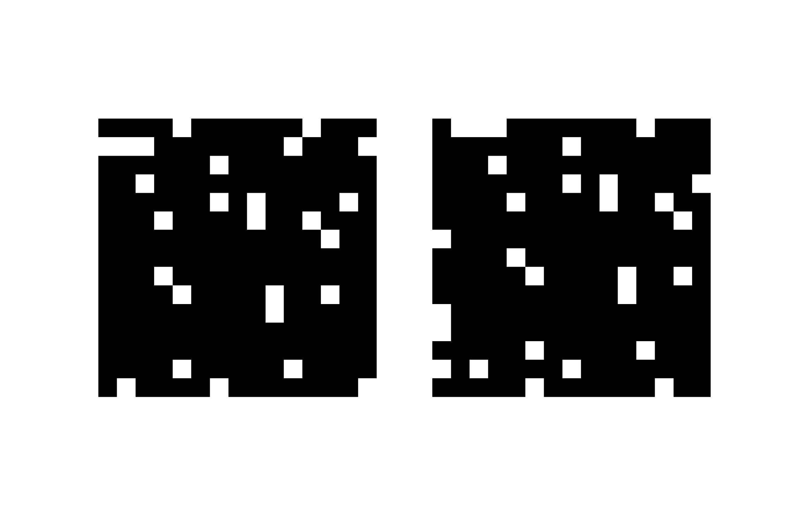
(a)	(b)

Figure 7: (a) Relational auto-encoder. (b) Toy data commonly used to test relational models. There is no structure in the images, only in their relationship.

2.4.2 Symmetric training

In probabilistic terms, predictive training amounts to modeling the conditional distribution $p(\bm{y}|\bm{x})=\int_{\bm{z}}p(\bm{y},\bm{z}|\bm{x})\;d\bm{z}$. [43] show how modeling instead the joint distribution can make it possible to perform image matching, by allowing us to quantify how compatible any two images are under to the trained model.

Formally, modeling the joint amounts simply to changing the normalization constant of the three-way RBM to $Z=\sum_{\bm{x},\bm{y},\bm{z}}\exp\big{(}E(\bm{x},\bm{y},\bm{z})\big{)}$ (cf. previous section). Learning is more complicated, however, because the simplifying view of case-based modulation no longer holds. [43] suggest using three-way Gibbs sampling to train the model.

As an alternative to modeling a joint probability distribution, [29] show how one can instead use a relational auto-encoder trained symmetrically on the sum of the two predictive objectives

$$\sum_{j}\big{(}y_{j}^{\alpha}-\sum_{ik}w_{ijk}x_{i}^{\alpha}z_{k}^{\alpha})^{2}+\sum_{i}\big{(}x_{i}^{\alpha}-\sum_{jk}w_{ijk}y_{j}^{\alpha}z_{k}^{\alpha})^{2}$$ (14)

This forces parameters to be able to transform in both directions, and it can give performance similar to symmetrically trained, fully probabilistic models [29]. Like an auto-encoder, this model can be trained with gradient based optimization.

2.4.3 Learning higher-order within-image structure

Another reason for learning the joint distribution is that it allows us to model higher-order within-image structure (for example, [25, 39, 23]).

[39] apply a GBM to the task of modeling second-order within-image features, that is, features that encode pair-wise products of pixel intensities. They show that this can be achieved by optimizing the joint GBM distribution and using the same image as input $\bm{x}$ and as output $\bm{y}$. In contrast to [43], [39] suggest hybrid Monte Carlo to train the joint.

One can also combine higher-order models with standard sparse coding models, by using some hidden units to model higher-order structure and some to learn linear codes [38, 29].

2.4.4 Toy example: Motion extraction and analogy making

Figure 8 (a) shows a toy example of a gated Boltzmann machine applied to translations. The model was trained on images showing iid random dots where the output image $\bm{y}$ is a copy of the input image $\bm{x}$ shifted in a random direction. The center column in both plots in Figure 8 visualizes the inferred transformation as a vector field. The vector-field was produced by (i) inferring the transformation given the image pair (Eq. 8), (ii) computing the transformation from the inferred hiddens, and (iii) finding for each input-pixel the output-position it is most strongly connected to [30]. The two right-most columns in both plots show how the inferred transformation can be applied to new images by analogy, that is, by computing the output-image given a new input image and the inferred transformation (Eq. 9). Figure 8 (b) shows an example, where the transformations are split-screen translations, that is, translations which are independent in the top half vs. the bottom half of the image. This illustrates how the model has to decompose transformations into factorial constituting transformations.

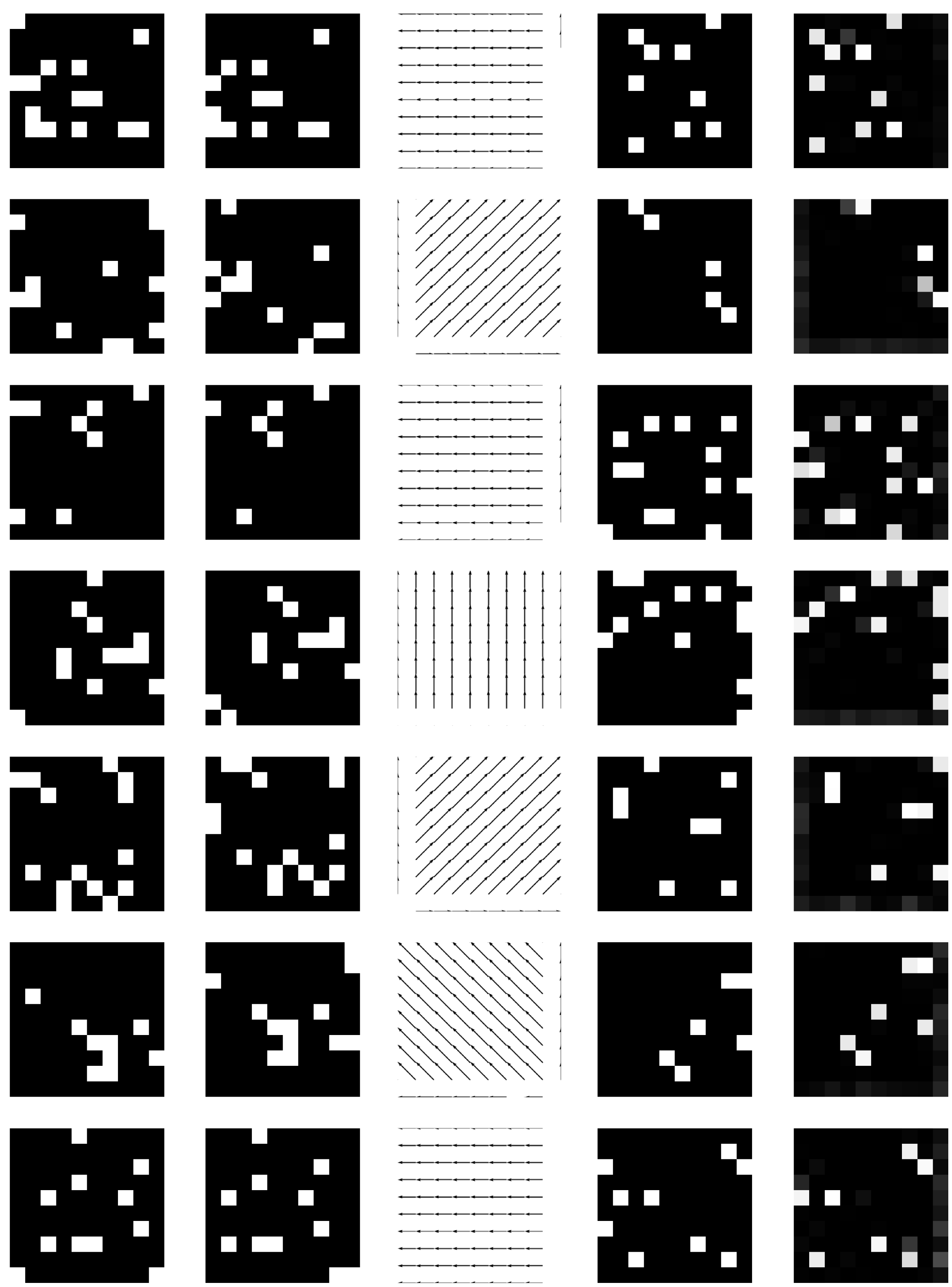
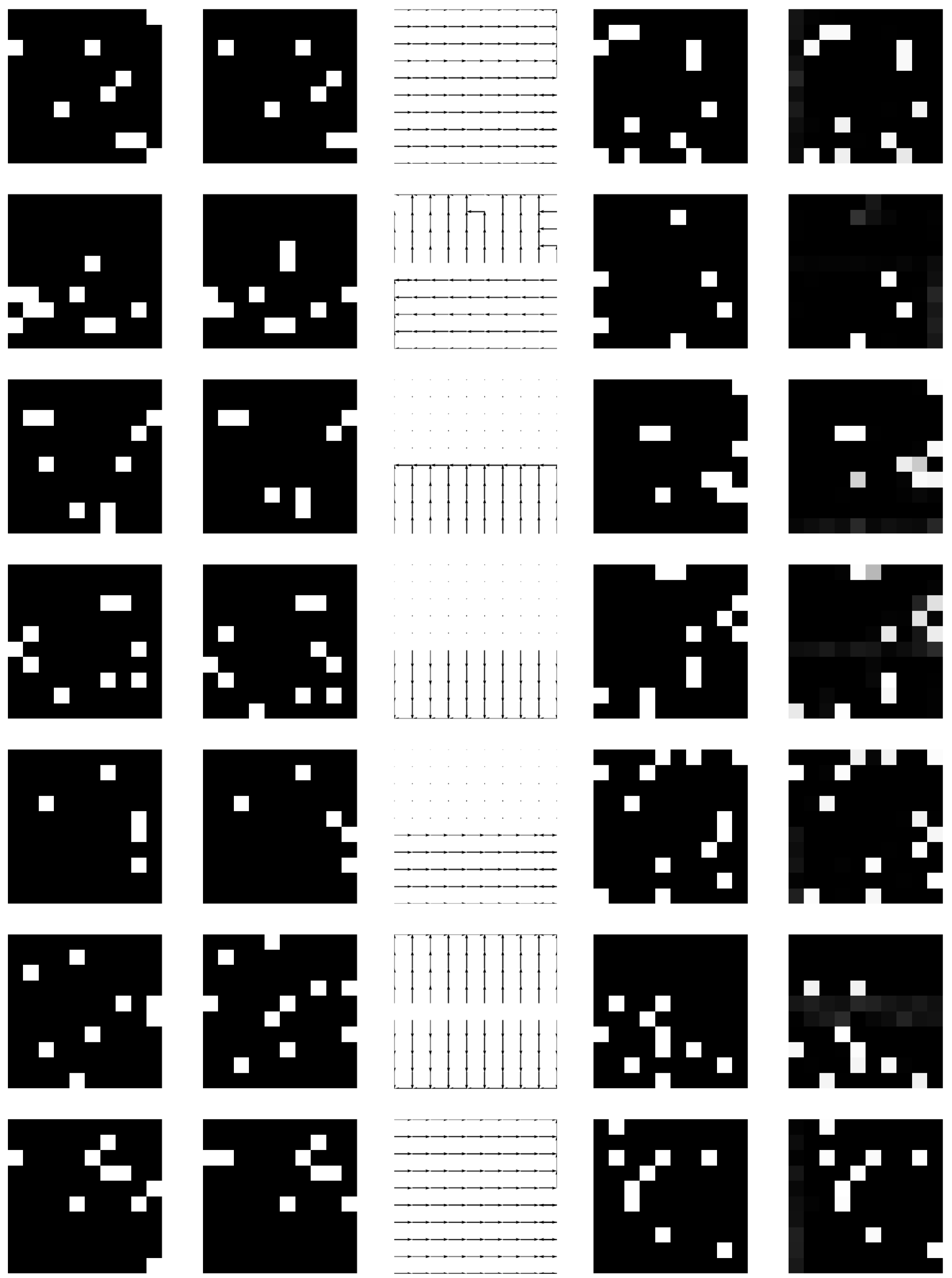
(a)	(b)

Figure 8: Inferring motion direction from test data. (a) Coherent motion across the whole image. (b) “Factorial motion” that is independent in different image regions. In both plots, the meaning of the five columns is as follows (left-to-right): Random test images $\bm{x}$, random test images $\bm{y}$, inferred flow-field, new test-image $\hat{\bm{x}}$, inferred output $\hat{\bm{y}}$.

3 Factorization and energy models

In the following, we discuss the close relationship between gated sparse coding models and energy models. For this end, we first describe how parameter factorization makes it possible to pre-process input images and thereby reduce the number of parameters.

3.1 Factorizing the gating parameters

The number of gating parameters is roughly cubic in the number of pixels, if we assume that the number of constituting transformations is about the same as the number of pixels. It can easily be more for highly over-complete hiddens. [31] suggest reducing that number by factorizing the parameter tensor $W$ into three matrices, such that each component $w_{ijk}$ is given by the “three-way inner product”

$$w_{ijk}=\sum_{ijk}\sum_{f=1}^{F}w^{x}_{if}w^{y}_{jf}w^{z}_{kf}$$ (15)

Here, $F$ is a number of hidden “factors”, which, like the number $K$ of hidden units, has to be chosen by hand or by cross-validation. The matrices $w^{x}$, $w^{y}$ and $w^{z}$ are $I\times F$, $J\times F$ and $K\times F$, respectively.

An illustration of this factorization is given in Figure 9 (a). It is interesting to note that, under this factorization, the activity of output-variable $y_{j}$, by using the distributive law, can by written:

$$y_{j}=\sum_{ik}w_{ijk}x_{i}z_{k}=\sum_{ik}(\sum_{f}w^{x}_{if}w^{y}_{jf}w^{z}_{kf})x_{i}z_{k}=\sum_{f}w^{y}_{jf}(\sum_{i}w^{x}_{if}x_{i})(\sum_{k}w^{z}_{kf}z_{k})$$ (16)

Similarly, for $z_{k}$ we have

$$z_{k}=\sum_{ij}w_{ijk}x_{i}y_{j}=\sum_{ij}(\sum_{f}w^{x}_{if}w^{y}_{jf}w^{z}_{kf})x_{i}y_{j}=\sum_{f}w^{z}_{kf}(\sum_{i}w^{x}_{if}x_{i})(\sum_{j}w^{y}_{jf}y_{j})$$ (17)

One can obtain a similar expression for the energy in a gated Boltzmann machine. Eq. 17 shows that factorization can be viewed as filter matching: For inference, each group of variables $\bm{x}$, $\bm{y}$ and $\bm{z}$ are projected onto linear basis functions which are subsequently multiplied, as illustrated in Figure 9 (b).

(a)	(b)

Figure 9: (a) Factorizing the parameter tensor. (b) Interpreting factorization as filter matching.

It is important to note that the way factorization reduces parameters is not by projecting data onto a lower-dimensional space before computing the multiplicative interactions – a claim that can be found frequently in the literature. In fact, frequently, $F$ is chosen to be larger than $I$ and/or $J$. The way that factorization reduces the number of parameters is by restricting three-way connectivity. Learning then amounts to finding basis functions that can deal with this restriction optimally. Using the factorization in Eq. 15 amounts to allowing each factor to engage only in a single multiplicative interaction.

All gated sparse coding models can be subjected to this factorization. Training is similar to training an unfactored model by using the chain rule and differentiating Eq. 15. An example of a factored gated auto-encoder is described in [29]. Virtually all factored models that were introduced use the restriction of single multiplicative interactions (Eq. 15). An open research question is to what degree a less restrictive connectivity – equivalently, using a non-diagonal core-tensor in the factorization – would be advantageous.

[31] show empirically how training factored model leads to filter-pairs that optimally represent transformation classes, such as Fourier-components for translations and a polar variant of Fourier-components for rotations. Figures 10 and 11 show examples of filters learned from translations, affine transformations, split-screen translations, which are independent in the top and bottom half of the image, and natural video. For training the filters in the top rows and on the bottom right, we used data-sets described in [31] and [29] and the model described in [29]. The filters resemble receptive fields found in various cells in visual cortex [10]. To obtain split-screen filters (bottom left) we generated a data-set of split-screen translations and trained the model described in [31]. In Section 4, we provide an analysis that sheds some light onto why the filters take on this form.

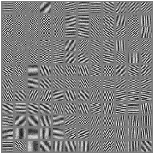
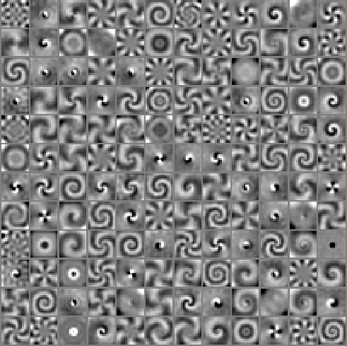
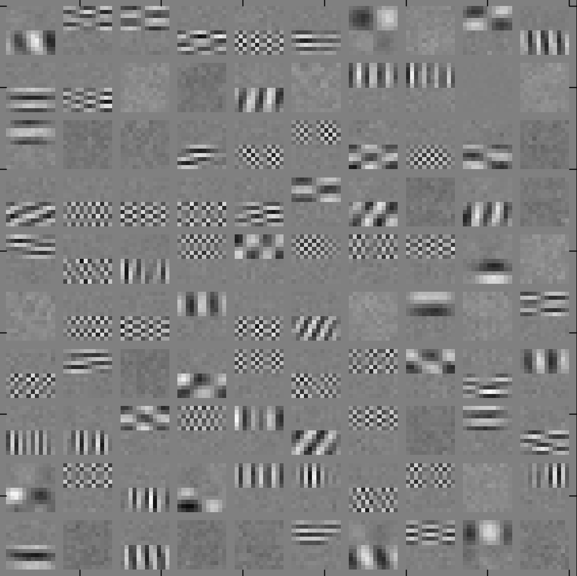
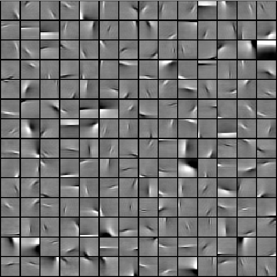
Figure 10: Input filters learned from various types of transformation. Top-left: Translation, Top-right: Rotation, Bottom-left: split-screen translation, Bottom-right: Natural videos. See figure 11 on the next page for corresponding output filters.

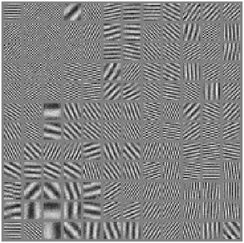
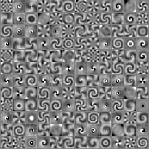
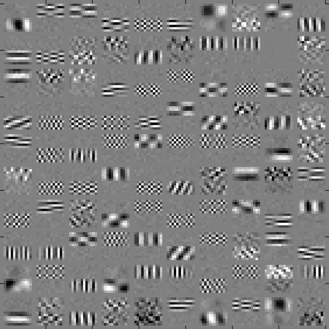
Figure 11: Output filters learned from various types of transformation. Top-left: Translation, Top-right: Rotation, Bottom-left: split-screen translation, Bottom-right: Natural videos. See figure 10 on the previous page for corresponding input filters.

3.2 Energy models

Energy models [1, 33] are an alternative approach to modeling image motion and disparities, and they have been deployed monocularly, too. A main application of energy models is the detection of small translational motion in image pairs. This makes them suitable as biologically plausible mechanisms of both local motion estimation and binocular disparity estimation. Energy models detect motion by projecting two images onto two phase-shifted Gabor functions each (for a total of four basis function responses). The two responses across the images are added and squared. The sum of these two squared, spatio-temporal responses then yields the response of the energy model.

The rationale behind the energy model is that, since each within-image Gabor filter pair can be thought of as a localized spatio-temporal Fourier component, the sum of the squared components yields an estimate of spectral energy, which is not dependent of the phase – and thus to a large degree not dependent on the content – of the input images. The two filters within each image need to be sine/cosine pairs, which is commonly referred to as being “in quadrature”.

A detector of local shift can be built by using a set of energy models tuned to different frequencies. To turn the set of energy responses into an estimate of local translation, one can, for example, pick the model with the strongest response [41, 37], or use pooling to get a more stable estimate [7].

Figure 12: Illustration of Independent Subspace Analysis applied to an image pair $(\bm{x},\bm{y})$.

[26, 23] suggest learning energy-like models from data by extending a sparse coding model with an elementwise squaring operation, followed by a linear pooling layer. In contrast to the original energy model, one may use more than exactly two filters to pool over, and pooling weights may be learned along with basis functions, instead of being fixed to be $1$. Figure 12 shows an illustration of this type of model applied to an image pair. As the figure shows, this type of model can be viewed as a two-layer network, with a hidden layer that uses an elementwise squaring nonlinearity.

For learning, [23] suggest adopting ICA by forcing the responses of latent variables (which are now sums of squared basis function responses) to be sparse, while keeping the filters orthogonal to avoid degenerate solutions, just like when training a standard ICA model (cf. Section 2.1). This approach is known as “Independent Subspace Analysis” (ISA). We shall refer to the hidden layer nodes as “factors” in analogy to the hidden layer of a factored GBM. Both ISA and factored gated Boltzmann machines were shown to yield state-of-the-art performance in various motion recognition tasks [27, 44].

3.3 Relationship between gated sparse coding and energy models

Learning energy models, such as ISA, on the concatenation of two inputs $\bm{x}$ and $\bm{y}$ is closely related to learning gated sparse coding models. Let $w_{\cdot f}^{x}$ ($w_{\cdot f}^{y}$) denote the set of weights connecting part $\bm{x}$ ($\bm{y}$) of the concatenated input with factor $f$ (cf. Figure 12). The activity of hidden unit $z_{k}$ in an energy model is given by

$$z_{k} = \sum_{f}w_{kf}^{z}\big{(}{w^{x}_{\cdot f}}^{\mathrm{T}}\bm{x}+{w^{y}_{\cdot f}}^{\mathrm{T}}\bm{y}\big{)}^{2}$$ (18)

$$= \sum_{f}w^{z}_{kf}\big{(}2({w^{x}_{\cdot f}}^{\mathrm{T}}\bm{x})({w^{y}_{\cdot f}}^{\mathrm{T}}\bm{y})+({w^{x}_{\cdot f}}^{\mathrm{T}}\bm{x})^{2}+({w^{y}_{\cdot f}}^{\mathrm{T}}\bm{y})^{2}\big{)}$$ (19)

Up to the quadratic terms in Eq. 19, hidden unit activities are the same as in a gated sparse coding model. As we shall discuss in detail below, the quadratic terms do not have a significant effect on the meaning of the hidden units. They can therefore also be thought of as a way to implement mapping units that encode relations.

3.4 Implementing gated sparse coding models

Over the years, a variety of tricks and recipes have emerged, which can simplify, stabilize, or speed up, learning in the presence of multiplicative interactions. One approach, that is used by practically everyone in the field, is to normalize output filter matrices $w^{x}$ and $w^{y}$ during learning, such that all filter $w^{x}_{\cdot f}$ and $w^{y}_{\cdot f}$ grow slowly and maintain roughly the same length as learning progresses. A common way to achieve this is to maintain a running average of the average norm of the filters during learning and to re-normalize each filter to have this norm after every learning update. Furthermore, it is common to connect top-level hidden units locally to the factors, rather than using full connectivity. The theoretical discussion in the next section provides some intuition into why local connectivity helps speed up learning. A slightly more complicated approach is to let all hidden units populate a virtual “grid” in a low-dimensional space (for example, 2-D) and to connect hidden units to factors, such that neighboring hidden units are connected to the same or to overlapping sets of factors. The approach has been popular mainly in the context of learning energy models (for example, [50, 24]). Finally, it is common to train the models using image patches that are DC centered and contrast normalized, and usually also whitened.

4 Relational codes and simultaneous eigenspaces

We now show that hidden variables learn to detect subspace-rotations when they are trained on transformed image pairs. In Section 2.3 (Eq. 10) we showed that transformation codes $\bm{z}$ can represent linear transformations, $L$, that is $\bm{y}=L\bm{x}$. We shall restrict our attention in the following to transformations, $L$, that are orthogonal, that is, $L^{\mathrm{T}}L=LL^{\mathrm{T}}=I$, where $I$ is the identity matrix. In other words, $L^{-1}=L^{\mathrm{T}}$. Linear transformations in “pixel-space” are also known as warp. Note that practically all relevant spatial transformations, like translation, rotation or local shifts, can be expressed approximately as an orthogonal warp, because orthogonal transformations subsume, in particular, all permutations (“shuffling pixels”).

An important fact about orthogonal matrices is that the eigen-decomposition $L=UDU^{\mathrm{T}}$ is complex, where eigenvalues (diagonal of $D$) have absolute value $1$ [20]. Multiplying by a complex number with absolute value $1$ amounts to performing a rotation in the complex plane, as illustrated in Figure 13 (left). Each eigenspace associated with $L$ is also referred to as invariant subspace of $L$ (as application of $L$ will keep eigenvectors within the subspace).

Figure 13: Training gated sparse coding models is equivalent to detecting rotation angles in the invariant subspaces associated with a set of transformations (left), and it amounts to detecting multiple applications of the same angle when learning from videos (right).

Applying an orthogonal warp is thus equivalent to (i) projecting the image onto filter pairs (the real and imaginary parts of each eigenvector), (ii) performing a rotation within each invariant subspace, and (iii) projecting back into the image-space. In other words, we can decompose an orthogonal transformation into a set of independent, 2-dimensional rotations. The most well-known examples are translations: A 1D-translation matrix contains ones along one of its secondary diagonals, and it is zero elsewhere. The eigenvectors of this matrix are Fourier-components [12], and the rotation in each invariant subspace amounts to a phase-shift of the corresponding Fourier-feature. This leaves the norm of the projections onto the Fourier-components (the power spectrum of the signal) constant, which is a well known property of translation.

It is interesting to note that the imaginary and real parts of the eigenvectors of a translation matrix correspond to sine and cosine features, respectively, reflecting the fact that Fourier components naturally come in pairs. These are commonly referred to as quadrature pairs in the literature. In the special case of Gabor features, the importance of quadrature pairs is that they allow us to detect translations independently of the local content of images [37, 7]. However, the property that eigenvectors come in pairs is not specific to translations. It is shared by all transformations that can be represented by an orthogonal matrix, so they can be composed from 2-dimensional rotations. [4] use the term generalized quadrature pair to refer to the eigen-features of these transformations.

4.1 Commuting warps share eigenspaces

A central observation to our analysis is that eigenspaces can be shared among transformations. When eigenspaces are shared, then the only way in which two transformations differ, is in the angles of rotation within the eigenspaces. So shared eigenspaces allow us to represent multiple transformations with a single set of features. An example of a shared eigenspace is the Fourier-basis, which is shared among translations. This well-known observation follows from the fact that the set of all circulant matrices (which are 1-D translation-matrices) of the same size have the Fourier-basis as eigen-basis [12]. Eigenspaces can be shared between many more transformation not just translation. An obvious generalization are local translations, which may be considered the constituting transformations of natural videos. Another, less obvious generalization is spatial rotation. Formally, a set of matrices share eigenvectors if they commute [20].

The importance of commuting transformations for our analysis is that, since these transformations share an eigen-basis, they differ only in the angle of rotation in the joint eigenspace. As a result, one may extract a particular transformation from a given image pair ($\bm{x},\bm{y}$) by recovering the angles of rotation between the projections of $\bm{x}$ and $\bm{y}$ onto the eigenspaces. For this end, consider the real and complex parts $\bm{v}_{\mathrm{R}}$ and $\bm{v}_{\mathrm{I}}$ of some eigen-feature $\bm{v}$. That is, $\bm{v}=\bm{v}_{\mathrm{R}}+i\bm{v}_{\mathrm{I}}$, where $i=\sqrt{-1}$. The real and imaginary coordinates of the projection of $\bm{x}$ onto the invariant subspace associated with $\bm{v}$ are given by $\bm{v}_{\mathrm{R}}^{\mathrm{T}}\bm{x}$ and $\bm{v}_{\mathrm{I}}^{\mathrm{T}}\bm{x}$, respectively. For the output image, they are $\bm{v}_{\mathrm{R}}^{\mathrm{T}}\bm{y}$ and $\bm{v}_{\mathrm{I}}^{\mathrm{T}}\bm{y}$.

Let $\phi_{x}$ and $\phi_{y}$ denote the angles of the projections of $\bm{x}$ and $\bm{y}$ with the real axis in the complex plane. If we normalize the projections to have unit norm, then the cosine of the angle between the projections, $\phi_{y}-\phi_{x}$, may be written

$$\cos(\phi_{y}-\phi_{x})=\cos\phi_{y}\cos\phi_{x}+\sin\phi_{y}\sin\phi_{x}$$

by trigonometric identity. This is equivalent to computing the inner product between two normalized projections (cf. Figure 13 (left)). In other words, to estimate the (cosine of) the angle of rotation between the projections of $\bm{x}$ and $\bm{y}$, we need to sum over the product of two filter responses.

Note, however, that normalizing each projection to $1$ amounts to dividing by the sum of squared filter responses, an operation that is highly unstable if a projection is close to zero. Unfortunately, this will be the case, whenever one of the images is almost orthogonal to the invariant subspace. This, in turn, means that the rotation angle cannot be recovered from the given image, because the image is too close to the axis of rotation. One may view this as a subspace-generalization of the well-known aperture problem beyond translation, to the set of orthogonal transformations. Normalization would ignore this problem and provide the illusion of a recovered angle even when the aperture problem makes the detection of the transformation component impossible. In the next section we discuss how one may overcome this problem by rephrasing the problem as a detection task.

4.2 Detecting subspace rotations

For each eigenvector, $\bm{v}$, and rotation angle, $\theta$, define the complex output image filter

$$\bm{v}^{\theta}=\exp(i\theta)\bm{v}$$

which represents a projection and simultaneous rotation by $\theta$. This allows us to define a subspace rotation-detector with preferred angle $\theta$ as follows:

$$r^{\theta}=(\bm{v}_{R}^{\mathrm{T}}\bm{y})({\bm{v}^{\theta}_{R}}^{\mathrm{T}}\bm{x})+(\bm{v}_{I}^{\mathrm{T}}\bm{y})({\bm{v}^{\theta}_{I}}^{\mathrm{T}}\bm{x})$$ (20)

where subscripts $R$ and $I$ denote the real and imaginary part of the filters like before. Like before, if projections are normalized to length $1$, we have

$$r^{\theta}=\cos\phi_{y}\cos(\phi_{x}-\theta)+\sin\phi_{y}\sin(\phi_{x}-\theta)=\cos(\phi_{y}-\phi_{x}-\theta),$$

which is maximal whenever $\phi_{y}-\phi_{x}=\theta$, thus when the observed angle of rotation, $\phi_{y}-\phi_{x}$, is equal to the preferred angle of rotation, $\theta$. However, like before, normalizing projections is not a good idea because of the subspace aperture problem. We now show that mapping units are well-suited to detecting subspace rotations, if a number of conditions are met.

4.3 Mapping units as rotation detectors

If features and data are contrast normalized, then the projections will depend only on how well the image pair represents a given subspace rotation. The value $r^{\theta}$, in turn, will depend (a) on the transformation (via the subspace angle) and (b) on the content of the images (via the angle between each image and the invariant subspace). Thus, the output of the detector factors in both, the presence of a transformation and our ability to discern it.

The fact that $r^{\theta}$ depends on image content makes it a suboptimal representation of transformation. However, note that $r^{\theta}$ is a “conservative” detector, that takes on a large value only if an input image pair $(\bm{x},\bm{y})$ is compatible with its transformation. We can therefore define a content-independent representation by pooling over multiple detectors $r^{\theta}$ that represent the same transformation but respond to different images. Note that computing $r^{\theta}$ involves summing over the two subspace dimensions, which is also a form of pooling (within subspaces). Thus, encoding subspace rotations requires two types of pooling.

If we stack imaginary and real eigenvector pairs for the input and output images, $\bm{v}$ and $\bm{v}^{\theta}$, in matrices $U$ and $V$, respectively, we may define the representation $\bm{t}$ of a transformation, given two images $\bm{x}$ and $\bm{y}$, as

$$\bm{t}=W^{\mathrm{T}}P\;\big{(}{U}^{\mathrm{T}}\bm{x}\big{)}\cdot\big{(}{V}^{\mathrm{T}}\bm{y}\big{)}$$ (21)

where $P$ is a band-diagonal “within-subspace” pooling matrix, and $W$ is an appropriate “across-subspace” pooling matrix. Furthermore, the following conditions need to be met: (1) Images $\bm{x}$ and $\bm{y}$ are contrast-normalized, (2) For each row $\bm{u}_{f}$ of $U$ there exists $\theta$ such that the corresponding row $\bm{v}_{f}$ of $V$ takes the form $\bm{v}_{f}=\exp(i\theta)\bm{u}_{f}$. In other words, filter pairs are related through rotations only.

Eq. 21 takes exactly the same form as inference in a gated sparse coding model (cf., Eq. 17), if we absorb the within-subspace pooling matrix $P$ into $W$. Learning amounts to identifying both the subspaces and the pooling matrix, so training a multi-view feature learning model can be thought of as performing multiple simultaneous diagonalizations of a set of transformations. When a data-set contains more than one transformation class, learning involves partitioning the set of orthogonal warps into commutative subsets and simultaneously diagonalizing each subset. Note that, in practice, complex filters can be represented by learning two-dimensional subspaces in the form of filter pairs. It is uncommon, albeit possible, to learn actually complex-valued features in practice.

Diagonalizing a single transformation, $L$, would amount to performing a kind of canonical correlations analysis (CCA), so learning a multi-view feature learning model may be thought of as performing multiple canonical correlation analyzes with tied features. Similarly, modeling within-image structure by setting $\bm{x}=\bm{y}$ [38] would amount to learning a PCA mixture with tied weights. In the same way that neural networks can be used to implement CCA and PCA up to a linear transformation, the result of training a multi-view feature learning model is a simultaneous diagonalization only up to a linear transformation.

It is interesting to note that condition (2) above implies that filters are normalized to have the same length. Imposing a norm constraint has been a common approach to stabilizing learning (eg., [38, 29, 43]). It is also common to apply a sigmoid non-linearity after computing mapping unit activities, so that the output of a hidden variable can be interpreted as a probability. Pooling over multiple subspaces may, in addition to providing content-independent representations, also help deal with edge effects and noise, as well as with the fact that learned transformations may not be exactly orthogonal.

5 Relation to energy models

By concatenating images $\bm{x}$ and $\bm{y}$, as well as filters $\bm{v}$ and $\bm{v}^{\theta}$, we may approximate the subspace rotation detector (Eq. 20) also with the response of an energy detector:

$$\begin{split}r^{\theta}&=\big{(}({\bm{v}_{R}}^{\mathrm{T}}\bm{y})+({\bm{v}^{\theta}_{R}}^{\mathrm{T}}\bm{x})\big{)}^{2}+\big{(}({\bm{v}_{I}}^{\mathrm{T}}\bm{y})+({\bm{v}^{\theta}_{I}}^{\mathrm{T}}\bm{x})\big{)}^{2}\\ &=2\big{(}({\bm{v}_{R}}^{\mathrm{T}}\bm{y})({\bm{v}^{\theta}_{R}}^{\mathrm{T}}\bm{x})+({\bm{v}_{I}}^{\mathrm{T}}\bm{y})({\bm{v}^{\theta}_{I}}^{\mathrm{T}}\bm{x})\big{)}\\ &+({\bm{v}_{R}}^{\mathrm{T}}\bm{y})^{2}+({\bm{v}^{\theta}_{R}}^{\mathrm{T}}\bm{x})^{2}+({\bm{v}_{I}}^{\mathrm{T}}\bm{y})^{2}+({\bm{v}^{\theta}_{I}}^{\mathrm{T}}\bm{x})^{2}\end{split}$$ (22)

Eq. 22 is equivalent to Eq. 20 up to the four quadratic terms. The four quadratic terms are equal to the sum of the squared norms of the projections of $\bm{x}$ and $\bm{y}$ onto the invariant subspace. Thus, like the norm of the projections, they contribute information about the discernibility of transformations. This makes the energy response more conservative than the cross-correlation response (Eq. 20). However, the peak response is still attained only when both images reside within the detector’s invariant subspace and when their projections are rotated by the detectors preferred angle $\theta$.

By pooling over multiple rotation detectors, $r^{\theta}$, we obtain the equivalent of an energy response (Eq. 18). This shows that energy models applied to the concatenation of two images are well-suited to modeling transformations, too.

5.1 More than two images

Both energy models and cross-correlation models can be applied to more than two images. For gated sparse coding, Eq. 20 can be modified to contain all cross-terms, or all the ones that are deemed relevant (for example, adjacent frames in a “Markov”-type gating model of a video). Alternatively, for the energy mechanism, one can compute the square of the concatenation of more than two images in place of Eq. 22.

5.1.1 Example: Implementing an energy model via cross-correlation

The close relation between energy models and gated sparse coding makes it possible to implement one via the other. Figure 14 shows example filters from an energy model trained on concatenated frames from videos showing moving random dots. We trained a gated auto-encoder with $F=256$ factors and $K=128$ mapping units, where $\bm{x}=\bm{y}$ is given by the concatenation of $10$ frames. Filters are constrained, such that $w^{x}_{if}=w^{y}_{if}$. Each $10$-frame input shows random dots moving at a constant speed. Speed and direction vary across movies.

Since the gated auto-encoder, a cross-correlation model, multiplies two sets of filter responses which are the same, it effectively computes a square, and thus implements an energy model. In the absence of any within-image structure, all filters learn to represent only across-image correlations. Thus, as predicted by Eq. 19 the energy model, in turn, implements a cross-correlation model.

Figure 14 depicts, separately, the $10$ sets of $256$ filters corresponding to the $10$ time-frames. It shows that the model learns spatio-temporal Fourier features which are selective for speed, frequency and orientation.

Frame: 1	2	3	4
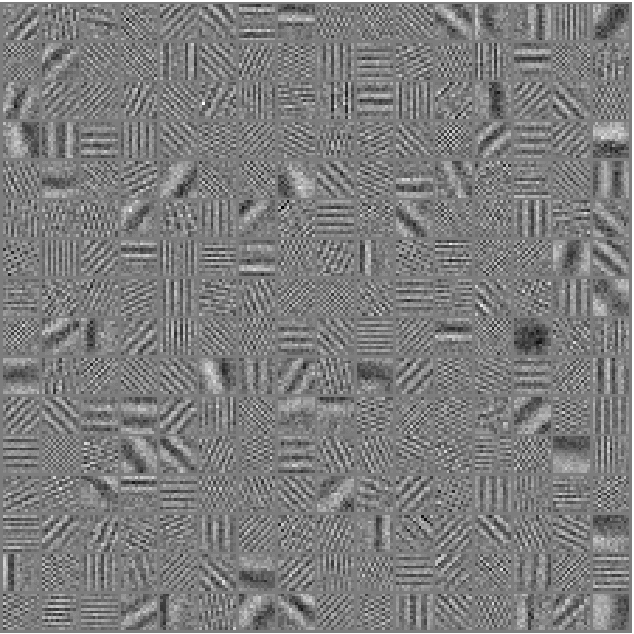
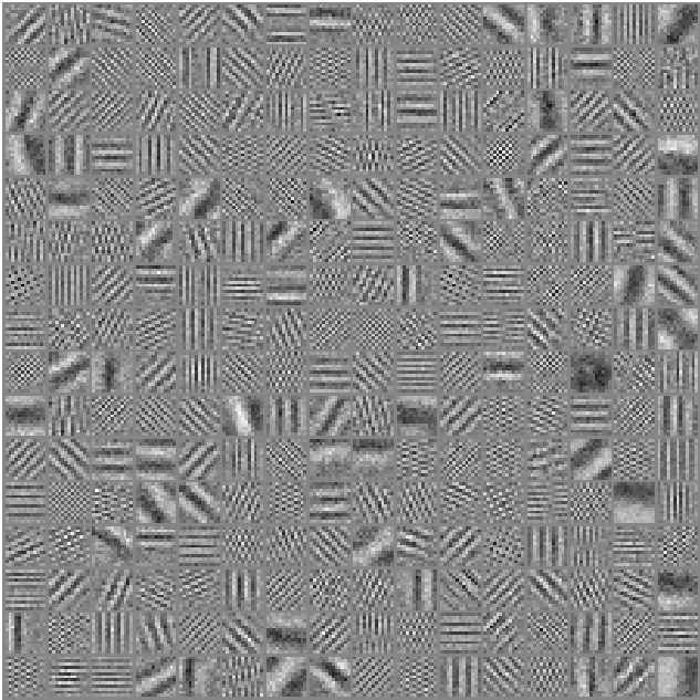
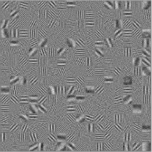
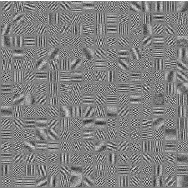
5	6	7	8
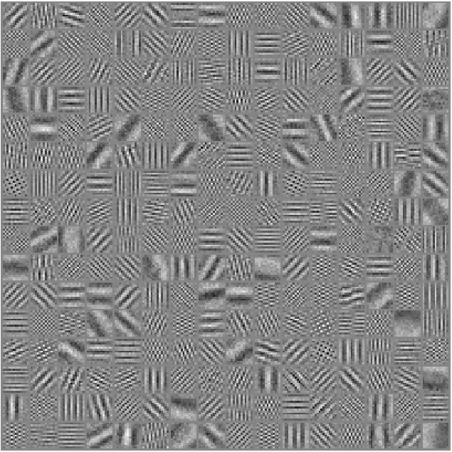
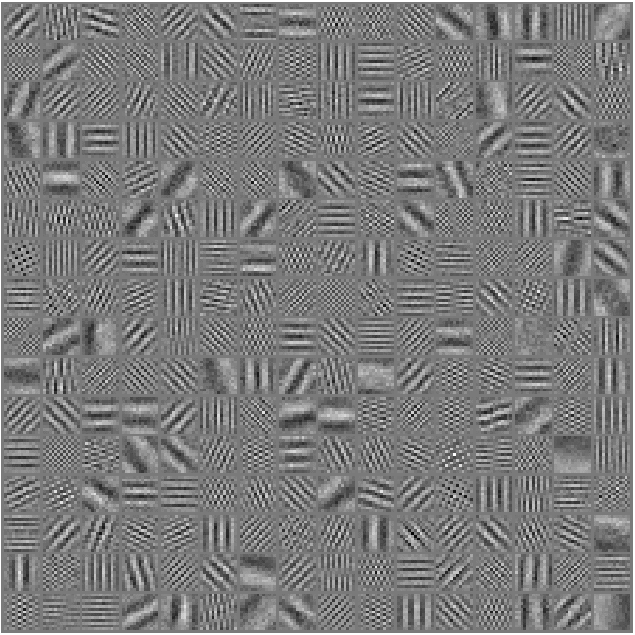
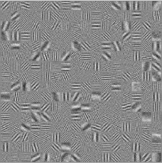
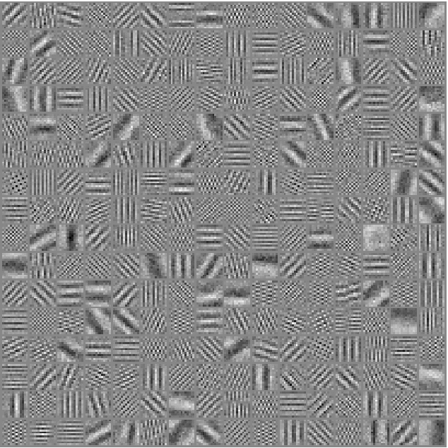
9	10

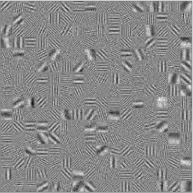
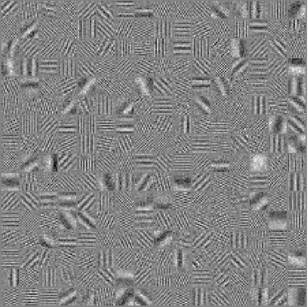
Figure 14: Implementing a cross-correlation model via an energy model via a cross-correlation model. Sequence of filters learned from the concatenation of $10$ frames of moving random dots.

6 Discussion

Given the predominance of correspondence tasks in vision, it seems conceivable that the main utility of energy models and complex cells is that they can encode relationships not (monocular) invariances.

This suggests that squaring non-linearities, for example, as the transfer function in a feed-forward network, may be useful, in general, in tasks where relations play a role, such as in recognition tasks that involve motion and stereo. In the long term, computing squares and/or cross-products could help reduce the requirement for large, hand-engineered pipelines, which are currently used for solving correspondence problems in tasks like depth inference. These typically involve keypoint extraction, descriptor extraction, matching and outlier-removal [14]. A learning based system using complex cells may be able to replace parts of the pipeline with a single, homogeneous model that is trained from data. This may also help explain how visual cortex may perform a large variety of tasks using a single, homogeneous module, which can be trained by a single type of learning mechanism.

Interestingly, invariant object recognition itself can be viewed as a correspondence problem, where the goal is to match an input observation to invariant templates in memory. [32] discuss a variation of a gated sparse coding model, which may be considered as an approach to invariant recognition through modeling mappings that take images to class labels. The input of the model is an image, the output is an orthogonal encoding of a class label, and prediction amounts to marginalizing over the set of possible mappings. The graphical model is also equivalent to a set of class-conditional manifolds or probability distributions, but inference is feed-forward. The model effectively transforms an input into a canonical pose, so that it can be matched with a template, which itself represents the object in some canonical pose. This can help explain the similarity, in general, between filters that allow for invariant recognition and those that allow for selective recognition of transformations. [32] show how “swirly features” similar to the rotation features in Figures 10 and 11 emerge when learning to perform rotationally invariant recognition. [3] showed that similar features can emerge in feed-forward recognition models that contain squaring non-linearities.

Most common object recognition systems are somewhat unrealistic in that they are trained to recognize single, static views of objects. Real biological systems get to see “movies” of objects that constantly move around or change their relative pose. It is interesting to note that a model that computes squares or cross-products could automatically learn to associate object identity with 3-D structure or with articulated motion, simply by being trained on multiple, concatenated frames.

Using multiplicative interactions can also be related to analogy making [31]. It can be argued that analogy making is at the heart of many cognitive phenomena [19]. An interesting question is, to what degree an analogy-making module could be a useful building block in models of higher-level cognitive capabilities. Since gated sparse coding and energy models can be trained with standard, even Hebbian-like, learning (cf., Section 2.2), analogy-making does not require any uncommon or unusual machinery besides multiplicative interactions.

Squaring can be approximated using other non-linearities (see, for example, [51] for a discussion). A possible research question is, what type of approximations of computing squares or cross-products may be advantageous computationally and/or more plausible biologically. Of course, squares could be simulated using a layer of a feed-forward network with sigmoid activations [9]. However, the abundance of matching and correspondence tasks in vision may provide some inductive bias in favor of genuine multiplicative interactions or squares.

Another research question is to what degree deviating from exactly commuting transformations and exactly orthogonal matrices hampers our ability to learn something useful. Existing experiments (for example in [30, 31]) suggest that there is some robustness, but there has been no quantitative analysis. It is conceivable, that one could pre-process data-points, such that they can be related through orthogonal matrices, in order to make them amenable to an energy or cross-correlation model. Interestingly, it seems that one way to do this, would be by transforming data to be high-dimensional and sparse.

References

- [1] E.H. Adelson and J.R. Bergen. Spatiotemporal energy models for the perception of motion. J. Opt. Soc. Am. A, 2(2):284–299, 1985.
- [2] P.A. Arndt, H.A. Mallot, and H.H. Bülthoff. Human stereovision without localized image features. Biological cybernetics, 72(4):279–293, 1995.
- [3] James Bergstra, Yoshua Bengio, and Jérôme Louradour. Suitability of V1 energy models for object classification. Neural Computation, pages 1–17, 2010.
- [4] M Bethge, S Gerwinn, and JH Macke. Unsupervised learning of a steerable basis for invariant image representations. In B. E. Rogowitz, editor, Human Vision and Electronic Imaging XII, pages 1–12, Bellingham, WA, USA, February 2007. SPIE.
- [5] Adam Coates, Honglak Lee, and A. Y. Ng. An analysis of single-layer networks in unsupervised feature learning.
- [6] Aaron Courville, James Bergstra, and Yoshua Bengio. A spike and slab restricted boltzmann machine. In Artificial Intelligence and Statistics, 2011.
- [7] D. Fleet, H. Wagner, and D. Heeger. Neural encoding of binocular disparity: Energy models, position shifts and phase shifts. Vision Research, 36(12):1839–1857, June 1996.
- [8] B. N. Flury. Common principal components in k groups. Journal of the American Statistical Association, 79(388):892–898, 1984.
- [9] K. Funahashi. On the approximate realization of continuous mappings by neural networks. Neural Netw., 2:183–192, May 1989.
- [10] J. L. Gallant, J. Braun, and D. C. Van Essen. Selectivity for polar, hyperbolic, and cartesian gratings in macaque visual cortex. Science, 259:1001–4, 1993.
- [11] C. Lee Giles and Tom Maxwell. Learning, invariance, and generalization in high-order neural networks. Appl. Opt., 26(23):4972–4978, December 1987.
- [12] Robert M. Gray. Toeplitz and circulant matrices: a review. Commun. Inf. Theory, 2:155–239, August 2005.
- [13] David Grimes and Rajesh Rao. Bilinear sparse coding for invariant vision. Neural Computation, 17(1):47–73, 2005.
- [14] R. I. Hartley and A. Zisserman. Multiple View Geometry in Computer Vision. Cambridge University Press, ISBN: 0521540518, second edition, 2004.
- [15] Fritz Heider and Marianne Simmel. An Experimental Study of Apparent Behavior. The American Journal of Psychology, 57(2):243–259, 1944.
- [16] Geoffrey E. Hinton. Training products of experts by minimizing contrastive divergence. Neural Computation, 14(8):1771–1800, 2002.
- [17] Geoffrey E. Hinton, Simon Osindero, and Yee-Whye Teh. A fast learning algorithm for deep belief nets. Neural Comput., 18:1527–1554, July 2006.
- [18] Geoffrey F. Hinton. A parallel computation that assigns canonical object-based frames of reference. In Proceedings of the 7th international joint conference on Artificial intelligence - Volume 2, pages 683–685, San Francisco, CA, USA, 1981.
- [19] Douglas R. Hofstadter. The copycat project: An experiment in nondeterminism and creative analogies. Massachusetts Institute of Technology, 755, 1984.
- [20] Roger A. Horn and Charles R. Johnson. Matrix Analysis. Cambridge University Press, 1990.
- [21] Patrik Hoyer and Aapo Hyvärinen. A multi-layer sparse coding network learns contour coding from natural images. Vision Research, 42:1593–1605, 2002.
- [22] A. Hyvarinen, J. Hurri, , and Patrik O. Hoyer. Natural Image Statistics: A Probabilistic Approach to Early Computational Vision. Springer Verlag, 2009.
- [23] Aapo Hyvärinen and Patrik Hoyer. Emergence of phase- and shift-invariant features by decomposition of natural images into independent feature subspaces. Neural Comput., 12:1705–1720, July 2000.
- [24] Aapo Hyvärinen, Patrik O. Hoyer, and Mika Inki. Topographic ica as a model of natural image statistics. In Seong-Whan Lee, Heinrich H. Bülthoff, and Tomaso Poggio, editors, Biologically Motivated Computer Vision, volume 1811 of Lecture Notes in Computer Science, pages 535–544. Springer, 2000.
- [25] Y. Karklin and M. S. Lewicki. Is early vision optimized for extracting higher-order dependencies? In Advances in Neural Information Processing Systems 18. MIT Press, 2006.
- [26] Teuvo Kohonen. The Adaptive-Subspace SOM (ASSOM) and its use for the implementation of invariant feature detection. In Proc. ICANN’95, Int. Conf. on Artificial Neural Networks, volume I, pages 3–10. EC2, 1995.
- [27] Q.V. Le, W.Y. Zou, S.Y. Yeung, and A.Y. Ng. Learning hierarchical spatio-temporal features for action recognition with independent subspace analysis. In Proc. CVPR, 2011. IEEE, 2011.
- [28] Roland Memisevic. Non-linear latent factor models for revealing structure in high-dimensional data. dissertation, University of Toronto, 2008.
- [29] Roland Memisevic. Gradient-based learning of higher-order image features. In Proceedings of the International Conference on Computer Vision (ICCV), 2011.
- [30] Roland Memisevic and Geoffrey Hinton. Unsupervised learning of image transformations. In Proceedings of IEEE Conference on Computer Vision and Pattern Recognition, 2007.
- [31] Roland Memisevic and Geoffrey E Hinton. Learning to represent spatial transformations with factored higher-order Boltzmann machines. Neural Computation, 22(6):1473–92, 2010.
- [32] Roland Memisevic, Christopher Zach, Geoffrey Hinton, and Marc Pollefeys. Gated softmax classification. In Advances in Neural Information Processing Systems 22. MIT Press, 2010.
- [33] Izumi Ohzawa, Gregory C. Deangelis, and Ralph D. Freeman. Stereoscopic Depth Discrimination in the Visual Cortex: Neurons Ideally Suited as Disparity Detectors. Science (New York, N.Y.), 249(4972):1037–1041, August 1990.
- [34] B. Olshausen and D. Field. Emergence of simple-cell receptive field properties by learning a sparse code for natural images. Nature, 381(6583):607–609, June 1996.
- [35] Bruno Olshausen. Neural Routing Circuits for Forming Invariant Representations of Visual Objects. PhD thesis, Computation and Neural Systems, 1994.
- [36] Bruno Olshausen, Charles Cadieu, Jack Culpepper, and David Warland. Bilinear models of natural images. In SPIE Proceedings: Human Vision Electronic Imaging XII, San Jose, 2007.
- [37] Ning Qian. Computing stereo disparity and motion with known binocular cell properties. Neural Comput., 6:390–404, May 1994.
- [38] Marc’Aurelio Ranzato and Geoffrey E. Hinton. Modeling Pixel Means and Covariances Using Factorized Third-Order Boltzmann Machines. In Computer Vision and Pattern Recognition, pages 2551–2558, 2010.
- [39] Marc’Aurelio Ranzato, Alex Krizhevsky, and Geoffrey E. Hinton. Factored 3-Way Restricted Boltzmann Machines For Modeling Natural Images. In Proc. Thirteenth International Conference on Artificial Intelligence and Statistics (AISTATS), 2010.
- [40] D. E. Rumelhart, G. E. Hinton, and J. L. Mcclelland. A general framework for parallel distributed processing. In Parallel distributed processing: explorations in the microstructure of cognition, volume 1, chapter 2, pages 45–76. MIT Press, 1986.
- [41] T. Sanger. Stereo disparity computation using Gabor filters. Biological Cybernetics, 59:405–418, 1988. 10.1007/BF00336114.
- [42] Paul Smolensky. Tensor product variable binding and the representation of symbolic structures in connectionist systems. Artificial Intelligence, 46:159–216, 1990.
- [43] J. Susskind, R. Memisevic, G. Hinton, and M. Pollefeys. Modeling the joint density of two images under a variety of transformations. In Proceedings of IEEE Conference on Computer Vision and Pattern Recognition, 2011.
- [44] Graham, W. Taylor, Rob Fergus, Yann LeCun, and Christoph Bregler. Convolutional learning of spatio-temporal features. In Proc. European Conference on Computer Vision (ECCV’10), 2010.
- [45] Joshua Tenenbaum and William Freeman. Separating style and content with bilinear models. Neural Computation, 12(6):1247–1283, 2000.
- [46] N Troje and HH Bülthoff. Face recognition under varying poses: The role of texture and shape. Vision Research, 36(12):1761–1771, 6 1996.
- [47] Pascal Vincent, Hugo Larochelle, Yoshua Bengio, and Pierre-Antoine Manzagol. Extracting and composing robust features with denoising autoencoders. ICML ’08, New York, NY, USA, 2008. ACM.
- [48] Christoph von der Malsburg. The correlation theory of brain function. Internal report, 81-2, Max-Planck-Institut für Biophysikalische Chemie, Postfach 2841, 3400 Göttingen, FRG, 1981. Reprinted in E. Domany, J. L. van Hemmen, and K. Schulten, editors, Models of Neural Networks II, chapter 2, pages 95–119. Springer-Verlag, Berlin, 1994.
- [49] M. J. Wainwright and E. P. Simoncelli. Scale Mixtures of Gaussians and the Statistics of Natural Images. In Adv. Neural Information Processing Systems (NIPS*99), volume 12, pages 855–861, Cambridge, MA, 2000. MIT Press.
- [50] Max Welling, Geoffrey E. Hinton, and Simon Osindero. Learning Sparse Topographic Representations with Products of Student-t Distributions. In NIPS 2002, 2002.
- [51] Christoph Zetzsche and Ulrich Nuding. Nonlinear and higher-order approaches to the encoding of natural scenes. Network (Bristol, England), 16(2-3):191–221, 2005.