Spin-orbital phase synchronization in the magnetic field-driven electron dynamics in a double quantum dot.

Abstract

We study the dynamics of an electron confined in a one-dimensional double quantum dot in the presence of driving external magnetic fields. The orbital motion of the electron is coupled to the spin dynamics by spin orbit interaction of the Dresselhaus type. We derive an effective time-dependent Hamiltonian model for the orbital motion of the electron and obtain a synchronization condition between the orbital and the spin dynamics. From this model we deduce an analytical expression for the Arnold tongue and propose an experimental scheme for realizing the synchronization of the orbital and spin dynamics.

I Introduction

Phase synchronization and related phenomena are among the most fascinating effects of nonlinear dynamics. Besides the deep fundamental interestLanda ; Glass ; Anishchenko ; Rulkov ; Pikovsky ; Osipov ; Kozlov , phase synchronization has a broad range of applications in chemistry Kocarev , ecology Peng , astronomy Pavlov , in the field of information transfer using chaotic signals Fradkov , and for the control of high frequency electronic devices Strogatz . In nonlinear dissipative systems, phase synchronization occurs if the frequency of the external driving field is close to the eigenfrequency of the system. In this case, for a certain frequency interval of the driving field the oscillations of the nonlinear dissipative system can be synchronized with the perturbing force. Usually, for stronger driving fields the frequency interval for the synchronization becomes broader and the synchronization protocol is more efficient. The broad and growing interest in the phase synchronization calls for the analysis of new possible realizations of this phenomenon. A particularly interesting issue is the application of the synchronization protocols for magnetic nanostructures, which have rich applications Fradkov ; Strogatz ; Hirjibehedin ; Rusponi ; Mirkovic ; Stroscio and exhibit interesting nonlinear dynamical properties that can be exploited as a testing ground for dynamical systems Chotorlishvili ; Schwab .

A principal challenge in nanoscience is to find an efficient procedure for the manipulation of the systems states. A high level of accuracy on the state control is required especially in such applications as quantum computing, where a precise tailoring of the entangled states is highly desirable Raimond ; Shevchenko . With this in mind several physical systems were considered up to now, e. g. Josephson junction qubits and Rydberg atoms in a quantum cavities Raimond ; Shevchenko , ion traps Zahringer , single molecular nanomagnets Wernsdorfer , and nanoelectromechanical resonators Heinrich ; Karabalin . Among others, one of the most promising systems are electron spins confined in two-dimensional quantum dots Valin-Rodriguez ; Levitov ; Rashba and in one-dimensional nanowires and nanowire-based quantum dots Pershin ; Romano ; Lu ; Crisan . The key element of the corresponding models is the spin orbit (SO) coupling term, which is linear in the electron momentum. Such momentum-dependent coupling offers a new way of manipulating the spin by changing the electron momentum via a periodic electric field. This is the idea of the electric-dipole spin resonance proposed by Rashba and Efros for the electrons confined in nanostructures on the scale of 10 nm Rashba . However, the external electric field can strongly affect the orbital dynamics and thus the system is driven out of the linear regime Khomitsky . The nonlinearities usually result in a complex behavior of the affected systems and their dynamics might become complicated and even unpredictable. On the other hand, the nonlinearity may also lead to a number of interesting phenomena. In spite of the huge interest in the systems with SO coupling, the influence of the spin dynamics on the orbital motion was not addressed yet in full detail. With the present work we would like to bridge this gap. Our goal is to investigate the possibilities of controlling the orbital motion of the electron via external magnetic fields acting on its spin and via the spin-orbit coupling. That can be considered as opposite to the electric-dipole spin resonance protocol proposed by Rashba and Efros Rashba . We will demonstrate that: (i) by using an external driving field one can achieve a sufficient degree of control over the orbital motion, and (ii) as a result, one can devise a very efficient synchronization protocol of the orbital motion and the spin dynamics based on the application of a pulsed external magnetic field.

II Theoretical model

We consider a model system of a single electron confined in a double quantum dot described by a potential of the form $U(x)=U_{0}\left[-2\left({x}/{d}\right)^{2}+\left({x}/{d}\right)^{4}\right]$. Here $U_{0}$ is the energy barrier separating two minima with $2d$ being the distance between them. We assume the system is dissipative, and the dissipation is a thermal effect appearing due to a coupling to environment. The dissipation, which impacts mainly on the orbital motion, is essential for the synchronization processes we are going to discuss later in the text. For strong driving magnetic fields, the influence of the dissipation on the spin dynamics is negligibly small and can be ignored. In addition, we assume that the temperature is low enough to prevent the activated over-the-barrier motion. For the particular value of $U_{0}\sim 20$ meV the low-temperature regime means $T<100$ K. For the GaAs-based structure with the electron effective mass $m$ being 0.067 of the free electron mass and $d\sim 100$ nm, the tunneling probability is small and a classical consideration is justified. To quantify the SO interaction we use a coupling term of the Dresselhaus type $H_{\rm so}=\alpha P_{x}\sigma^{x}$, where $P_{x}$ is the momentum of the electron and $\sigma^{x}$ is the Pauli matrix. Therefore, the Hamiltonian of the one dimensional system reads:

$$H=\frac{P_{x}^{2}}{2m}+U(x)+\alpha P_{x}\sigma^{x}+\mu_{B}gB_{z}(t)\frac{\sigma^{z}}{2}+\mu_{B}gB_{x}(t)\frac{\sigma^{x}}{2},$$ (1)

where $\mu_{B}$ is the Bohr magneton and $g$ is the electron Landé factor. Here $B_{z}(t)=B_{0}\sum\limits_{t=0}^{\infty}\delta_{\tau}(t-nT)$ is an infinite series of external magnetic field pulses with the pulse strength $B_{0}$, which is applied along the $z$ axis. The temporal width of the pulses applied along the $z$-axis is smaller than the interval between the pulses $\tau\ll T$ (in what follows we set $T=1$). On the other hand, for the pulses along the $x$-axis $B_{x}(t)=B_{0}\sum\limits_{t=0}^{\infty}\Delta_{T}(t-\tau n)$ the pulse duration is larger than interval between pulses $T\ll\tau$ (cf. Fig. 1). A different route to the control of the spin-dynamics in double quantum dots via electric field pulses is outlined in jonas .

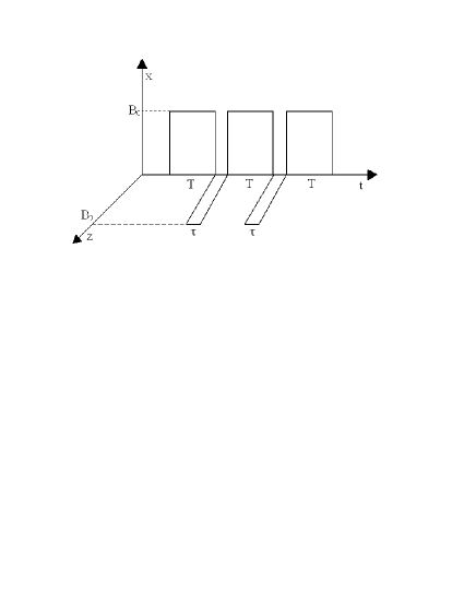
Figure 1: Schematic illustration of the infinite series of external magnetic field pulses applied to the system. A series of the short pulses $B_{z}(t)=B_{0}\sum\limits_{t=0}^{\infty}\delta_{\tau}(t-nT)$ with the pulse width $\tau$ and time interval between pulses $T$, is applied along the $z$ axis. Series of the pulses with the larger width $T$ and a shorter interval between the pulses $\tau$, $B_{x}(t)=B_{0}\sum\limits_{t=0}^{\infty}\Delta_{T}(t-\tau n)$ is applied along the $x$ axis. The amplitude of the pulses $B_{0}$ is the same in both cases.

Introducing the characteristic maximum momentum of the electron $P_{x}^{\max}=\sqrt{2mU_{0}}$ we can estimate the maximal precession rate of the spin due to the SO coupling $\Omega_{\rm so}^{\max}=({2\alpha}/{\hbar})\sqrt{2mU_{0}}$, while the magnetic field pulse of the amplitude $B=B_{0}$ induces a spin precession with the rate $\Omega_{B}={\mu_{B}|g|B_{0}}/{\hbar}$. Therefore, if $\Omega_{B}>\Omega_{\rm so}^{\max}$ we can during the pulse neglect the spin rotation produced by the SO coupling and the spin is completely controlled by the external driving fields. We need a protocol with two driving fields in order to fulfill the synchronization requirements as discussed later in the text. Namely, for the control of the spin dynamics via the external driving fields, the amplitudes of the fields should be large, $B_{0}>({2\alpha}/{\mu_{B}|g|})\sqrt{2mU_{0}}$. On the other hand, a strong constant magnetic field produces a high frequency precession of the spin $\Omega_{B}={\mu_{B}|g|B_{0}}/{\hbar}$, while for the synchronization we need to tune the precession frequency up or down keeping fixed the strong driving field amplitude. Below we will show that the optimal conditions for the synchronization are realized using two types of the driving pulses. Applying short pulses along the $z$-axis $\tau\ll T$, $B_{z}(t)=B_{0}\sum\limits_{t=0}^{\infty}\delta_{\tau}(t-nT)$ and long pulses along the $x$-axis $B_{x}(t)=B_{0}\sum\limits_{t=0}^{\infty}\Delta_{T}(t-\tau n)$, we can realize a spin precession with a frequency, which is inversely proportional to the time interval between the short pulses $\Omega\sim 1/T$ independently from the driving field strength $B_{0}$. In what follows, for convenience we use dimensionless units via the transformations $E\rightarrow E/4U_{0}$, $x\rightarrow x/d$, $t\rightarrow t\sqrt{{4U_{0}}/{m}}$, $P_{x}\rightarrow{P_{x}}/{\sqrt{2mU_{0}}}$, $\varepsilon\rightarrow\alpha/4U_{0}$.

III Dissipative system and the problem of phase synchronization between orbital and spin motion

III.1 Spin dynamics in pulsed magnetic fields

As was stated above the synchronization can occur if the frequency of the driving field is close to the eigenfrequency of the nonlinear dissipative system. If this is the case, in the particular frequency interval, the oscillations of the nonlinear dissipative system and the field can be synchronized. With the increase in the driving field amplitude, the synchronization can occur in a broader frequency interval, and the synchronization protocol becomes more efficient. Our aim is to develop a method for the synchronization of the dynamics of the electron spin and the orbital motion, using an external driving magnetic field and SO coupling. Although the magnetic field is not coupled to the orbital motion directly, a sufficiently strong field influences the orbital motion through the spin dynamics if the SO coupling is present. If SO term is relatively small $\Omega_{\rm so}^{\max}<\Omega_{B}$, that is

$$\Omega_{B}=\frac{\mu_{B}|g|B_{0}}{\hbar}>\Omega_{\rm so}^{\max}=\frac{2\alpha}{\hbar}\sqrt{2mU_{0}},$$ (2)

the spin and, correspondingly, the orbital motion can be controlled externally. From Eq. (1) it is easy to see, that in between the short pulses the electron spin rotates around the $x$-axis and the equations of motion for the electron spin in this case read

$$\dot{\sigma}^{x}=0,\quad\dot{\sigma}^{y}=-\Omega_{B}\sigma^{z},\quad\dot{\sigma}^{z}=\Omega_{B}\sigma^{y}.$$ (3)

On the other hand, during the short pulses we have

$$\dot{\sigma}^{x}=-\Omega_{B}\sigma^{y},\quad\dot{\sigma}^{y}=\Omega_{B}\sigma^{x},\quad\dot{\sigma}^{z}=0.$$ (4)

Considering the dynamics due to the pulse acting on the spin at the moment of time $t=t_{0}$, we can split the evolution operator $\hat{T}_{\rm ev}$ defined as

$$\bm{\sigma}\left(t_{0}^{[-]}+T\right)=\hat{T}_{\rm ev}\bm{\sigma}\left(t_{0}^{[-]}\right)$$ (5)

into two parts: $\hat{T}_{\rm ev}=\hat{T}_{R}\times\hat{T}_{\delta}$, where

$$\bm{\sigma}\left(t_{0}^{[+]}\right)=\hat{T}_{\delta}\bm{\sigma}\left(t_{0}^{[-]}\right),$$

$$\bm{\sigma}\left(t_{0}^{[-]}+T\right)=\hat{T}_{R}\bm{\sigma}\left(t_{0}^{[+]}\right).$$ (6)

Here we introduced the notations $t_{0}^{[+]}\equiv t_{0}+0$ and $t_{0}^{[-]}\equiv t_{0}-0$. The operator $\hat{T}_{R}$ describes the rotation of the electron spin around the $x$-axis produced by the long pulse of the external driving magnetic field $B_{x}(t)=B_{0}\sum\limits_{t=0}^{\infty}\Delta_{T}(t-\tau n)$, which is applied along the $x$ -axis and $\hat{T}_{\sigma}$ corresponds to the evolution produced by the short pulses $B_{z}(t)=B_{0}\sum\limits_{t=0}^{\infty}\delta_{\tau}(t-nT)$ applied along the $z$-axis. Integrating Eq. (4) for a short time interval $t\in\left(t_{0}^{[-]},t_{0}^{[+]}\right)$ we obtain

$$\hat{T}_{\delta}(\sigma^{x})=\sigma^{x}(t_{0}^{[-]})\cos(\Omega_{B}\tau)-\sigma^{y}(t_{0}^{[-]})\sin(\Omega_{B}\tau),$$ (7)

$$\hat{T}_{\delta}(\sigma^{y})=\sigma^{x}(t_{0}^{[-]})\sin(\Omega_{B}\tau)+\sigma^{y}(t_{0}^{[-]})\cos(\Omega_{B}\tau).$$ (8)

Integrating Eq. (3) during the time interval $t\in\left(t_{0}^{[+]},t_{0}^{[-]}+T\right)$ of long applied pulse we find

$$\hat{T}_{R}(\sigma^{y})=\sqrt{1-\left(\sigma^{x}\left(t_{0}^{[+]}\right)\right)^{2}}\cos(\Omega_{B}T),$$ (9)

$$\hat{T}_{R}(\sigma^{z})=\sqrt{1-\left(\sigma^{x}\left(t_{0}^{[+]}\right)\right)^{2}}\sin(\Omega_{B}T).$$ (10)

Combining Eq. (7) with Eq. (9) we finally can reconstruct the complete picture of the full time evolution of the electron spin:

$$\left\{\begin{array}[]{ll}\sigma_{n+1}^{y}=\sqrt{1-(\sigma_{n+1}^{x})^{2}}\cos((n+1)\Omega_{B}T),\\ \sigma_{n+1}^{z}=\sqrt{1-(\sigma_{n+1}^{x})^{2}}\sin((n+1)\Omega_{B}T),\\ \sigma_{n+1}^{x}=\sigma_{n}^{x}\cos(\Omega_{B}\tau)-\sqrt{1-(\sigma_{n}^{x})^{2}}\sin(\Omega_{B}\tau)\cos(n\Omega_{B}T).\end{array}\right.$$ (11)

The recurrent relations Eq. (11) describe the spin dynamics. Accuracy of the employed approximations may be checked by the validity of the normalization condition ${\bm{\sigma}}^{2}=1.$ In order to identify, whether the nonlinear map (11) is chaotic or regular, we evaluate the Lyapunov exponent for the spin system Schuster . Taking into account the peculiarity of the system (11), which is the fact, that the equation for the $x$ component $\sigma_{n+1}^{x}$ is self-consistent $\sigma_{n+1}^{x}=f(\sigma_{n}^{x})$, we deduce for the Lyapunov exponent

$$\lambda(\sigma_{0}^{x})=\lim\limits_{N\rightarrow\infty\atop\delta\sigma\rightarrow 0}\frac{1}{N}\ln\left|\frac{f^{N}(\sigma_{0}^{x}+\delta\sigma)-f^{N}(\sigma_{0}^{x})}{\delta\sigma}\right|=\lim\limits_{N\rightarrow\infty}\frac{1}{N}\ln\left|\frac{df^{N}(\sigma_{0}^{x})}{d\sigma_{0}^{x}}\right|\,.$$ (12)

Here, $\sigma_{0}^{x}$ is the initial value of the spin projection and the small increment of the initial values $\sigma_{0}^{x}+\delta\sigma$ quantifies the sensitivity of the recurrence relations (11) with respect to the slight change in the initial conditions. After some algebra from Eqs. (11) and (12) we finally obtain:

$$\lambda(\sigma_{0}^{x})=\lim\limits_{N\rightarrow\infty}\frac{1}{N}\sum\limits_{n=0}^{N-1}\ln\left|\frac{df(\sigma_{n}^{x})}{d\sigma_{n}^{x}}\right|=\frac{1}{N}\sum\limits_{n=0}^{N-1}\ln\left|\cos(\Omega_{B})+\frac{\sigma_{n}^{x}}{\sqrt{1-(\sigma_{n}^{x})^{2}}}\sin(\Omega_{B})\cos(n\Omega_{B})\right|\,.$$ (13)

The results of the numerical calculations are presented on Figs. 2 and 3.

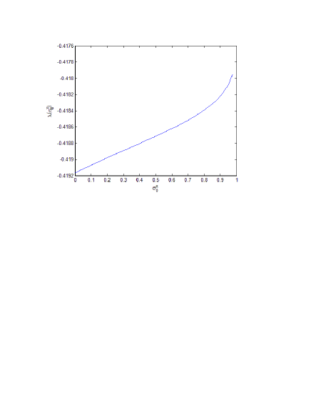
Figure 2: Lyapunov exponent as a function of the initial spin component $\sigma_{0}^{x}$. After $N=1000$ iterations the Lyapunov exponent is negative $\lambda(\sigma_{0}^{x})<0$, meaning that the spin dynamics is regular. $T=1$, $\Omega_{B}\tau=1$, $\Omega_{B}T=20$. At these conditions, the dependence is weak.

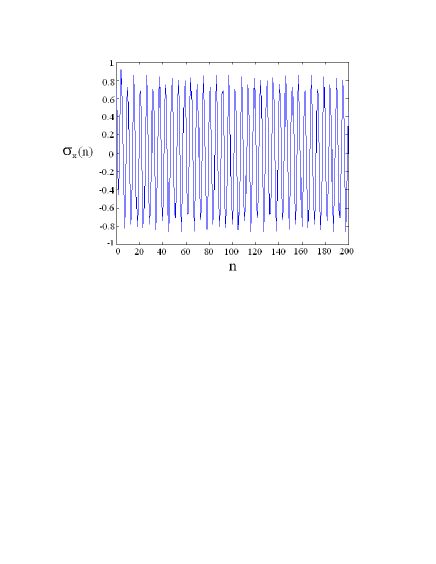
Figure 3: Time dependence of the spin projection $\sigma_{n}^{x}\equiv\sigma^{x}(n)$. $T=1$, $\Omega_{B}\tau=1$, $\Omega_{B}T=20$. From Fig. 3 we see that $\sigma_{n}^{x}=\sigma^{x}(t)$ is periodic in time and the frequency of oscillations $\Omega$ is inversely proportional to the time lapse between pulses $\Omega\approx 1/T$.

From Fig. 2 we see that the Lyapunov exponent is negative, $\lambda(\sigma_{0}^{x})<0$ and therefore the spin dynamics is regular, since the initial distance between two neighboring trajectories starting from the initial points $\sigma^{x}_{0}$ and $\sigma^{x}_{0}+\delta\sigma$ is not increasing asymptotically after an infinite number of iterations $\delta\sigma e^{N\lambda(\sigma_{0})}$. Therefore, from Figs. 2 and 3 we conclude, that the dynamics of the electron spin is controlled by the magnetic field pulses, thus following equation $\sigma^{x}(t)=\sigma^{x}_{0}\cos(\Omega t)$ we achieve the spin manipulation by magnetic fields. The spin rotation frequency is determined by the time interval between the short pulses $\Omega\approx 1/T$.

III.2 Synchronization of the spin and the orbital motion.

With the spin dynamics discussed in the previous subsection, for the orbital motion of electron we can write the following effective Hamiltonian assuming that $\sigma^{x}(t)\approx\cos(\Omega t)$:

$$H=\frac{P_{x}^{2}}{2m}+U(x)+\alpha P_{x}\cos(\Omega t).$$ (14)

The equation of motion for the system (14) has the form:

$$\ddot{x}+\gamma\dot{x}-x+x^{3}=-\beta\sin(\Omega t)\,,$$ (15)

where two new dimensionless quantities are introduced: $\beta={\alpha\Omega m}/{4U_{0}}$ and $\gamma\rightarrow\gamma/4U_{0}m$. We seek a solution of Eq. (15) using the following ansatz

$$x(t)=\frac{1}{2}A(t)e^{i\Omega t}+\frac{1}{2}A^{*}(t)e^{-i\Omega t}\,.$$ (16)

Assuming that the amplitude $A(t)$ in Eq. (16) is a slow variable the following condition applies

$$\dot{A}(t)e^{i\Omega t}+\dot{A}^{*}(t)e^{-i\Omega t}=0\,.$$ (17)

Taking into account Eqs. (16) and (17) from Eq. (15) we deduce:

$$i\Omega\dot{A}(t)e^{i\Omega t}-\left(\frac{\Omega^{2}}{2}A(t)e^{i\Omega t}+\mbox{c.c.}\right)+$$

$$+\gamma\left(\frac{i\Omega}{2}A(t)e^{i\Omega t}+\mbox{c.c.}\right)-\left(\frac{1}{2}A(t)e^{i\Omega t}++\mbox{c.c.}\right)+$$ (18)

$$+\frac{1}{8}\left(A^{3}(t)e^{3i\Omega t}+3|A(t)|^{2}A(t)e^{i\Omega t}+\mbox{c.c.}\right)=\frac{\beta}{2i}\left(e^{i\Omega t}-\mbox{c.c.}\right)\,.$$

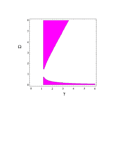
Figure 4: Arnold tongue diagram in terms of the decay constant $\gamma$ and field frequency $\Omega$, plotted using the conditions (25). Shadowed regions define parameter values for which the synchronization is possible.

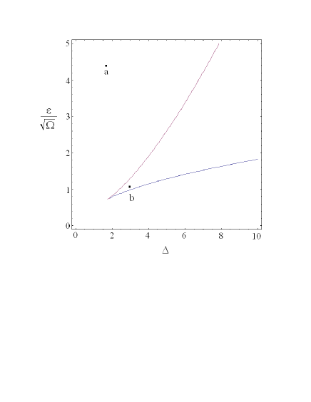
Figure 5: Arnold tongue in terms of the parameters $\Delta=\left(\Omega^{2}+1\right)/{\gamma\Omega}$, $(\Delta,\varepsilon)$ plotted using Eq. (26). Point $b$ belongs to the domain where a synchronization is not possible, while $a$ belongs to the synchronization domain.

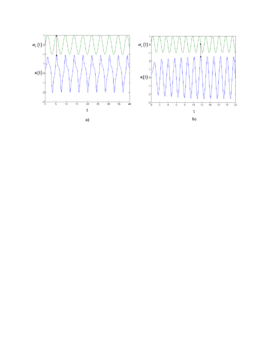
Figure 6: Orbital and spin dynamics plotted using the exact numerical integration of the Eq. (15). Panel a) corresponds to the values of parameters for which a synchronization is possible (see Fig. 5, point a). In particular $\left({\varepsilon}/{\sqrt{\Omega}}=4.41,\Delta=1.88\right)$. The right panel b) corresponds to the point b on Fig.5, $\left({\varepsilon}/{\sqrt{\Omega}}=1.05,\Delta=3.03\right)$, i.e. the dynamics occurs outside of the synchronization area. We see that in the former case the orbital and the spin dynamics are in phase and in the latter case the phase difference is about $\pi/2$ .

Multiplying Eq. (III.2) by the exponent $e^{-i\Omega t}$ and averaging it over the fast phases we find:

$$\dot{A}(t)+\frac{(\Omega^{2})+1)i}{2\Omega}A(t)+\frac{\gamma}{2}A(t)-\frac{3i}{8\Omega}|A(t)|^{2}A(t)=-\frac{\beta}{2\Omega}.$$ (19)

Introducing the notations

$$A(t)=2\sqrt{\gamma}z(t),\quad\tau=\frac{t\gamma}{2},\quad\Delta=\frac{\Omega^{2}+1}{\gamma\Omega},\quad\varepsilon=\frac{\beta}{2\Omega\gamma^{3/2}},$$ (20)

we can rewrite Eq. (19) in a more compact form

$$\dot{z}(\tau)+i\Delta z(\tau)=-z(\tau)+\frac{3i}{\Omega}|z(\tau)|^{2}z(\tau)+\varepsilon.$$ (21)

Inserting $z(\tau)=R(\tau)e^{i\varphi(\tau)}$ into Eq. (21), for the real and imaginary parts we obtain

$$\left\{\begin{array}[]{ll}\dot{R}(\tau)=-R+\varepsilon\cos\varphi(\tau),\\ \dot{\varphi}(\tau)+\Delta=\displaystyle{\frac{3}{\Omega}}R^{2}(\tau)-\displaystyle{\frac{\varepsilon}{R(\tau)}}\sin\varphi(\tau).\end{array}\right.$$ (22)

Using Eq. (22) and setting $\dot{R}=0$, $\dot{\varphi}=0$ for the stationary solutions we obtain:

$$f(\xi)=\xi+\xi\left(\frac{3}{\Omega}\xi-\Delta\right)^{2}=\varepsilon^{2},$$ (23)

$$\xi_{1,2}=\frac{\Omega}{9}\left(2\Delta\pm\sqrt{\Delta^{2}-3}\right)\,,$$ (24)

where $R^{2}=\xi$ and $\xi_{1,2}$ are roots of the equation ${df(\xi)}/{d\xi}=0$. In order to identify the Arnold tongue Kuznetsov , which shows the regions in which a synchronization is possible, we utilize the standard condition ${df(\xi)}/{d\xi}=0$. From Eq. (24) it is not difficult to see that the roots of the equation ${df(\xi)}/{d\xi}=0$ are real if $\Delta>\sqrt{3}$. Taking into account that $\Delta=\left(\Omega^{2}+1\right)/{\gamma\Omega}$ we can rewrite the inequality in the form $\Omega^{2}+1>\gamma\Omega\sqrt{3}$. Consequently we obtain the following criteria for the synchronization

$$0<\Omega<\frac{1}{2}(\gamma\sqrt{3}-\sqrt{3\gamma^{2}-4}),\quad\Omega>\frac{1}{2}(\gamma\sqrt{3}+\sqrt{3\gamma^{2}-4}),\quad\gamma>\frac{2}{\sqrt{3}}$$ (25)

Graphical representation of the conditions (25) is shown in Fig. 4.

Eq. (25) defines the synchronization area in terms of the external field frequency $\Omega$ and the dissipation constant $\gamma$. The minima points of the function $f(\xi)$, (23) does not depend on the SO coupling constant $\alpha$. Therefore criteria (25) is independent of the values of the SO coupling strength as well. Nevertheless, inserting the roots $\xi_{1,2}$ of the equation ${df(\xi)}/{d\xi}=0$ into Eq. (23) one can derive more illustrative and precise criteria in the form of the parametrical curve:

$$\frac{2}{81}(\pm 3\sqrt{\Delta^{2}-3}+9\Delta+\Delta^{3}\mp\Delta^{2}\sqrt{\Delta^{2}-3})-\left(\frac{\varepsilon}{\sqrt{\Omega}}\right)^{2}=0.$$ (26)

The parametrical curve defined by Eq. (26) represents the border of the synchronization domain, see Fig. 5. Taking into account that $\beta={\alpha\Omega m}/{4U_{0}}$, $\varepsilon={\beta}/{2\Omega\gamma^{3/2}}$ we obtain

$$\frac{\varepsilon}{\sqrt{\Omega}}=\frac{\alpha}{\sqrt{\Omega}}\frac{m}{8U_{0}\gamma^{3/2}}.$$ (27)

From Eq. (27) we see that the parameters of Fig. 5 depend on the oscillation frequency that can be easily controlled by tuning the time interval between pulses $\Omega\approx 1/T$. All other parameters in Eq. (27), such as the SO coupling constant $\alpha$, barrier height $U_{0}$, and the electron effective mass $m$ are internal characteristics of the system whereas the decay constant $\gamma$ is related to the thermal effects. Using Eq. (26) and Fig. 5 one can synchronize the electron orbital motion with its spin dynamics.

IV Conclusions.

We have investigated the classical electron dynamics in a double dot potential, with the spin of electron being controlled by external magnetic fields. We have shown that the orbital electron dynamics can be controlled very effectively by the field in the presence of a spin-orbit coupling. Using the proposed protocol of magnetic field pulses of different duration we have shown that it is possible to synchronize the spin and the orbital motion of the electron. In particular, if the driving field amplitude is large enough, $B_{0}>({2\alpha}/{\mu_{B}|g|})\sqrt{2mU_{0}}$, the spin dynamics is periodical in time. Then $\sigma^{x}(t)=\sigma^{x}_{0}\cos(\Omega t)$, where the oscillation frequency is inversely proportional to the time interval between pulses $\Omega\approx 1/T$ and can be tuned independently from the amplitude of the pulses $B_{0}$. As a consequence the orbital dynamics can be studied with reduced effective, time-dependent, one-dimensional model. By using this model we found the synchronization condition between the orbital and the spin dynamics. Furthermore, we derived an analytical expression for the Arnold tongue that defines the values of the parameters for which a synchronization is possible. Since in the designed protocol the spin precession rate is determined by the interval between the applied pulses we believe that it can be realized in future experiments on semiconductor quantum dot devices.

Acknowledgments The financial support by the Deutsche Forschungsgemeinschaft (DFG) through SFB 762, and contract BE 2161/5-1, Grant No. KO-2235/3, and STCU Grant No. 5053 is gratefully acknowledged. EYS acknowledges support of the MCI of Spain grant FIS2009-12773-C02-01, and ”Grupos Consolidados UPV/EHU del Gobierno Vasco” grant IT-472-10.

References

- (1) P. S. Landa and A. Rabinovitch, Phys. Rev. E 61, 1829 (2000).
- (2) L. Glass, Nature 410, 277 (2001).
- (3) V. S. Anishchenko and A. N. Pavlov, Phys. Rev. E 57, 2455 (1998)
- (4) N. F. Rulkov, M. A. Vorontsov, and L. Illing, Phys. Rev. Lett. 89, 277905 (2002).
- (5) A. Pikovsky, M. Rosenblum, J. Kurths, and S. Strogatz, Physics Today 56, 47 (2003).
- (6) G. V. Osipov, A. Pikovsky, and J. Kurths, Phys. Rev. Lett. 88, 054102 (2002).
- (7) A. K. Kozlov, M. M. Sushchik, Ya. I. Molkov, and A. S. Kuznetsov, Int. J. Bifurcation and Chaos 9, 2271 (1999).
- (8) L. Kocarev and U. Parlitz, Phys. Rev. Lett. 74, 5028 (1995).
- (9) J.H. Peng, E. J. Ding, M. Ding, and W. Yang, Phys. Rev. Lett. 76, 904 (1996).
- (10) V. Anishchenko, S. Nikolaev, and J. Kurths, Phys. Rev. E 76, 046216 (2007).
- (11) A. L. Fradkov, B. Andrievsky, and R. Evans, Phys. Rev. E 73 066209 (2006).
- (12) S. H. Strogatz, Nonlinear Dynamics and Chaos: with Applications to Physics, Biology, Chemistry, and Engineering (Reading, Mass. Addison-Wesley, 1994).
- (13) C. F. Hirjibehedin, C. P. Lutz, and A. J. Heinrich, Science 312, 1021 (2006).
- (14) S. Rusponi, T. Cren, N. Weiss, M. Epple, P. Buluschek, L. Claude, and H. Brune, Nat. Mater. 2, 546 (2003).
- (15) T. Mirkovic, M. L. Foo, A. C. Arsenault, S. Fournier-Bidoz, N. S. Zacharia, and G. A. Ozin, Nat. Nanotechnol. 2, 565 (2007).
- (16) J. A. Stroscio and R. J. Celotta, Science 306, 242 (2004).
- (17) L. Chotorlishvili, Z. Toklikishvili, A. Komnik, and J. Berakdar, Phys. Rev. B 83, 184405 (2011).
- (18) L. Chotorlishvili, P. Schwab, Z. Toklikishvili, and J. Berakdar, Phys. Rev. B 82, 014418 (2010).
- (19) J. Raimond, M. Brune, and S. Haroche, Rev. Mod. Phys. 73, 565 (2001).
- (20) S.N. Shevchenko, S. Ashhab, and F. Nori, Phys. Rep. 492, 1 (2010).
- (21) F. Zahringer, G. Kirchmair, R. Gerritsma, E. Solano, R. Blatt, and C.F. Roos, Phys. Rev. Lett. 104, 100503 (2010).
- (22) W. Wernsdorfer, N. Aliaga-Alcalde, D. N. Hendrickson, and G. Christou, Nature 416, 406 (2002).
- (23) G. Heinrich and F. Marquardt, EPL 93, 18003 (2011).
- (24) R. B. Karabalin, M. C. Cross, and M. L. Roukes, Phys. Rev. B 79, 165309 (2009).
- (25) M. Valin-Rodriguez, A. Puente, L. Serra, and E. Lipparini, Phys. Rev. B 66, 235322 (2002).
- (26) L. S. Levitov and E. I. Rashba, Phys. Rev. B 67, 115324 (2003).
- (27) E. I. Rashba and Al. L. Efros, Phys. Rev. Lett. 91, 126405 (2003).
- (28) Y. V. Pershin, J. A. Nesteroff, and V. Privman, Phys. Rev. B 69, 121306 (2004).
- (29) C. L. Romano, P. I. Tamborenea, and S. E. Ulloa, Phys. Rev. B 74, 155433 (2006).
- (30) C. Lü, U. Zülicke, and M. W. Wu, Phys. Rev. B 78, 165321 (2008).
- (31) M. Crisan, D. Sánchez, R. López, L. Serra, and I. Grosu, Phys. Rev. B 79, 125319 (2009).
- (32) D. V. Khomitsky and E. Ya. Sherman, Phys. Rev. B 79, 245321 (2009).
- (33) J. Waetzel, A. S. Moskalenko, and J. Berakdar, arXiv:1103.5866.
- (34) H. G. Schuster, Deterministic Chaos, An Introduction (VCH-Verlagsgesellschaft-Physik Verlag, Weinheim, 1985).
- (35) A.P. Kuznetsov, S.P. Kuznetsov, and N.M. Ryskin, Nonlinear Oscillations (Moscow, Fizmatlit, in Russian, 2002).