Magnetic and density spikes in cosmic ray shock precursors

Abstract

In shock precursors populated by accelerated cosmic rays (CR), the CR return current instability is believed to significantly enhance the pre-shock perturbations of magnetic field. We have obtained fully-nonlinear exact ideal MHD solutions supported by the CR return current. The solutions occur as localized spikes of circularly polarized Alfven envelopes (solitons, or breathers). As the conventional (undriven) solitons, the obtained magnetic spikes propagate at a speed $C$ proportional to their amplitude, $C=C_{A}B_{{\rm max}}/\sqrt{2}B_{0}$. The sufficiently strong solitons run thus ahead of the main shock and stand in the precursor, being supported by the return current. This property of the nonlinear solutions is strikingly different from the linear theory that predicts non-propagating (that is, convected downstream) circularly polarized waves. The nonlinear solutions may come either in isolated pulses (solitons) or in soliton-trains (cnoidal waves). The morphological similarity of such quasi-periodic soliton chains with recently observed X-ray stripes in Tycho supernova remnant (SNR) is briefly discussed. The magnetic field amplification determined by the suggested saturation process is obtained as a function of decreasing SNR blast wave velocity during its evolution from the ejecta-dominated to the Sedov-Taylor stage.

1 Introduction

The nonresonant cosmic ray (CR) return current instability (also termed as Bell’s instability) is expected to bootstrap the acceleration of CR in shocks by enhancing the magnetic field in the shock precursor. The most unstable is a circularly polarized, field aligned, aperiodic mode, similar to the internal kink (Kruskal-Shafranov) mode in plasmas (see, e.g., Ryutov et al., 2006). In the context of the CR acceleration in shocks, it was also studied by Achterberg (1983); Shapiro et al. (1998).

Bell (2004) reawakened the interest in this instability by emphasizing its role in magnetic field amplification and suggested its saturation due to magnetic tension. But, since the growth rate decreases with the wave number only as $\sqrt{k}$, the magnetic tension term does not stabilize the long waves. This opens the door for a strong, $\delta B\gg B_{0}$ field amplification. The caveat is that the non-propagating long waves have limited (precursor-crossing) time to grow. By contrast, the nonlinear solutions, that we present in this paper, can stand off in the flow ahead of the shock, thus warranting the saturation.

There have been considerable efforts to understand the Bell’s mode saturation mechanisms, with a strong emphasis on the MHD and PIC simulations (Bell, 2004; Pelletier et al., 2006; Vladimirov et al., 2006; Reville et al., 2007; Niemiec et al., 2008; Zirakashvili et al., 2008; Bykov et al., 2009; Luo & Melrose, 2009; Riquelme & Spitkovsky, 2009; Stroman et al., 2009; Dieckmann et al., 2010). As first demonstrated in 3D MHD simulations by Bell (2005) (see also Niemiec et al., 2008), the saturation is achieved when the Ampere force expels plasma and the helical magnetic field radially, thus forming plasma cavities. The instability appears to saturate only in 3D, or at least requires a quasi-2D dynamics, perpendicular to the ambient field. However, the fastest growing modes are field-aligned, i.e., at least initially one-dimensional. Therefore, it is necessary to understand structures that form at the 1D phase and particularly the nonlinear mechanisms of their saturation and propagation ahead of the shock. These structures may in the main cease to grow before the subsequent 3D dynamics kick in largely by spreading the saturated turbulence energy in $k$-space. Although this scenario may appear to be at odds with many simulations, recent Chandra observations of the Tycho supernova remnant (SNR), for example, indicate the presence of quasi-1D structures (stripes), inconsistent with the quasi-isotropic nonlinear dynamics observed in those simulations (Eriksen et al., 2011). Moreover, while being very useful for our understanding of CR instabilities, simulations cover only a tiny fraction of the dynamical range of typical SNR-shock acceleration process and introduce artificial dissipation in essentially collisionless plasmas.

Alfven waves usually saturate by modulational instability. However, being a strong MHD aperiodic instability, Bell’s instability hampers direct applications of standard methods, such as the weak-turbulence theory (Sagdeev & Galeev, 1969). The latter typically deals with propagating and weakly interacting eigen modes and, as a driver amplifies them, they cascade the wave energy to the dissipation scale. The Bell’s linear mode does not propagate (in the linear approximation), and does not even exists without the driving current. The lack of long wave stabilization is also based on the comparison of linear contributions to the square of the growth rate of the driving current ($\propto k$) and magnetic tension ($\propto k^{2},$ eq.[12] below). A clue to saturation in a similar system of the pressure-anisotropy-driven fire-hose instability is provided by an exact solution due to Berezin & Sagdeev (1969). While at peaks of magnetic energy it takes nearly all the instability free energy ($B_{\perp}^{2}/8\pi\sim P_{\parallel}-P_{\perp}\gg B_{0}^{2}/8\pi$), on the average only the moderate field amplification $B_{\perp}\sim B_{0}$ is observed.

In this paper we present an exact solution of the current-driven MHD equations (e.g., CR return current). It differs from the linearly growing solution in that it propagates with the velocity proportional to its (constant) amplitude and is spatially localized.

2 Basic equations

The linear theory of Bell’s instability indicates that the fastest growing modes are directed along the ambient magnetic field (Bell, 2005). Therefore, we will consider 1D magnetohydrodynamic (MHD) equations in a CR shock precursor using a coordinate system with the axis $x$ along the field. The general 1D equations read:

$$\frac{d\rho}{dt}+\rho\frac{\partial}{\partial x}U_{x}=0,$$ (1)

$$\frac{dU_{x}}{dt}=-\frac{1}{\rho}\frac{\partial}{\partial x}\frac{B_{\perp}^{2}}{8\pi},$$ (2)

$$\frac{d\mathbf{U}_{\perp}}{dt}=\frac{B_{0}}{4\pi\rho}\frac{\partial\mathbf{B_{\perp}}}{\partial x}+\frac{1}{c\rho}\mathbf{J}\times\mathbf{B_{\mathbf{\perp}}},$$ (3)

$$\frac{d\mathbf{B}_{\perp}}{dt}=B_{0}\frac{\partial\mathbf{U}_{\perp}}{\partial x}-\mathbf{B}_{\perp}\frac{\partial U_{x}}{\partial x}.$$ (4)

Here $d/dt\equiv\partial/\partial t+U_{x}\partial/\partial x$, $\rho$ is the gas density, $U_{x}$,$B_{0}$ and $\mathbf{U_{\mathbf{\perp}}}$,$\mathbf{B}_{\perp}$ are the gas velocity and magnetic field components along the field and in the ($y,z$)-plane, respectively. The x-component of magnetic field $B_{x}=B_{0}=const$ because of $\nabla\cdot\mathbf{B=0}$. In eq.(3) we have included the plasma return current by representing the total plasma current as $\mathbf{J}_{tot}=\left(c/4\pi\right)\nabla\times\mathbf{B}+\mathbf{J}$, where the part of the plasma current $\mathbf{J=-}\mathbf{J}_{CR}$ compensates the CR current. Eq.(3) implies that in our reference frame $\mathbf{J}\times\mathbf{B}_{0}=0$. We neglect the thermal and CR pressure, as Bell (2004) did. It should be noted, however, that these CR pressure gradient drives an acoustic instability of the shock precursor (also called Drury’s instability, Drury, 1984; Dorfi, 1984). Moreover, the acoustic instability grows faster than the Bell’s instability for $\beta=8\pi P/B_{0}^{2}<1$ (see Malkov et al., 2010 where the studies of evolution, saturation, as well as the associated particle transport and cascading of magnetic energy, are also referenced).

Returning to eqs.(1-4), it is convenient to introduce a Lagrangian mass coordinate $\xi$:

$$d\xi=\frac{\rho}{\rho_{0}}\left(dx-U_{x}dt\right),$$ (5)

where $\rho_{0}$ is the background density. Considering scales shorter than the precursor size, we treat $\rho_{0}$ and the bulk plasma speed $U_{x0}$ as coordinate independent ($U_{x0}=0$ in the plasma frame).

Next, we reduce eqs.(1-4) to the following system of two equations that describe the magnetic field and density perturbations:

$$\frac{\partial^{2}}{\partial t^{2}}\frac{B}{\rho}-C_{A}^{2}\frac{\partial^{2}}{\partial\xi^{2}}\frac{B}{\rho_{0}} = \frac{i}{c\rho_{0}}B_{0}J\frac{\partial}{\partial\xi}\frac{B}{\rho}$$ (6)

$$\frac{\partial^{2}}{\partial t^{2}}\frac{\rho_{0}^{2}}{\rho}+\frac{\partial^{2}}{\partial\xi^{2}}\frac{\left|B\right|^{2}}{8\pi} = 0,$$ (7)

where

$$B=B_{y}+iB_{z}\;\;{\rm and}\;\;C_{A}^{2}=\frac{B_{0}^{2}}{4\pi\rho_{0}}.$$

The r.h.s. of eqs.(6) is the instability driver. Without it, the equations describe the conventional MHD modes, propagating at an arbitrary angle to the ambient magnetic field. By choosing the averaged components $\overline{B}_{y}=\overline{B}_{z}=0$, we restrict our treatment to the parallel propagation along the x-direction.

3 Traveling wave solutions

We look for the solutions of the system given by eqs.(6) and (7) in the form of a traveling wave:

$$B=B_{{\rm max}}v\left(\zeta\right)e^{-i\omega t}$$ (8)

$$\rho=\rho\left(\zeta\right)$$

where $\zeta=\xi-Ct$, $C$ is the (constant) propagation speed of the traveling wave, $B_{{\rm max}}$ is the wave amplitude that we specify in eq.(9) below, and $\omega=\Re\omega$ is the wave frequency. Note that for $\omega\neq 0$, the solution is not steady in any reference frame. For that reason, the spatially localized version of this solution is some times called ’breather’ as opposed to the soliton, customary to $\omega=0$ case. Integrating then eq.(7) twice, we obtain

$$\frac{\rho_{0}}{\rho}=1-\frac{\left|B\right|^{2}}{B_{{\rm max}}^{2}}$$ (9)

where $B_{{\rm max}}^{2}\equiv 8\pi\rho_{0}C^{2}$. We have chosen the integration constants in such a way that $B\to 0$ for $\rho\to\rho_{0}$ (background plasma) and $B\to B_{{\rm max}}$ for $\rho\to\infty$ (flow stagnation point, if present). This sets the interval for variation of $v\left(\zeta\right):\;0<v<1$.

Substituting $B$ from eq.(8) and $\rho$ from the last equation, eq.(6) yields

$$\frac{\partial^{2}}{\partial\zeta^{2}}\left(a-\left|v\right|^{2}\right)v-iK\frac{\partial}{\partial\zeta}\left(1-\left|v\right|^{2}\right)v-\frac{\omega^{2}}{C^{2}}\left(1-\left|v\right|^{2}\right)v=0.$$ (10)

Here we have used the following notations

$$K=\frac{B_{0}J}{c\rho_{0}C^{2}}-2\frac{\omega}{C},\;\;a=1-2\frac{B_{0}^{2}}{B_{max}^{2}}=1-\frac{C_{A}^{2}}{C^{2}},$$ (11)

where $C_{A}^{2}=B_{0}^{2}/4\pi\rho_{0}$. The linear dispersion relation can be recovered by letting $v\left(\zeta\right)\propto e^{ik\zeta}$, $v\to 0$ in eq.(10):

$$\omega=kC\pm\sqrt{k^{2}C_{A}^{2}+B_{0}Jk/c\rho_{0}}.$$ (12)

The arbitrary propagation speed $C$ is a parameter of a Galilean transformation (zero in the plasma frame), while the imaginary part of $\omega$ is an invariant of such transformation as it should be. In the nonlinear treatment the wave velocity with respect to the plasma depends on the wave amplitude (nonlinear dispersion relation). Meanwhile, the linear instability occurs in the long wave limit for $B_{0}Jk<0$. It should be emphasized that only if the quadratic $B$ term is neglected in eq.(9), is there no coupling to the density modulations in eq.(6). It is interesting to note that in the strong nonlinear limit $B_{max}/B_{0}\to\infty$, eq.(10) degenerates into a linear equation for the function $v\left(1-\left|v\right|^{2}\right)$. This limit, however, cannot be understood without the nonlinear solution.

To find such solution, we write

$$v\left(\zeta\right)=\sqrt{w}e^{i\Theta}$$ (13)

where $w\left(\zeta\right)\geq 0$. Substituting $v$ from eq.(13) into eq.(10) and separating the imaginary part, for the phase $\Theta$ we obtain the following equation:

$$\frac{d\Theta}{ds}=\frac{wP\left(w\right)+A}{w(a-w)^{2}},$$ (14)

where

$$P\equiv w^{2}-(3a+1)w/2+a$$

We have introduced a new variable $s=K\zeta/2$ and an integration constant $A$. We may choose it by specifying the properties of the solution sought. The regularity of $\Theta$ at $w=0$ implies $A=0$. Next, taking the real part of eq.(10) and using eq.(14) with $A=0$, for $w\left(s\right)$ we obtain

$$\frac{d^{2}f}{ds^{2}}-\frac{w^{2}P^{2}}{f^{3}}+2\sqrt{w}\left(1-w\right)\left[\frac{wP}{f^{2}}-2\frac{\omega^{2}}{C^{2}K^{2}}\right]=0$$ (15)

where we have denoted

$$f\left(w\right)\equiv\sqrt{w}(a-w)$$

Eq.(15) can be readily integrated by multiplying it by $df/ds$. We choose the integration constant to select an isolated pulse (soliton) solution of eq.(15), i.e. $w\to 0,$ as $s\to\pm\infty$. Then, the first integral reads

$$\left(\frac{dw}{ds}\right)^{2}-\frac{w^{2}}{\left(3w-a\right)^{2}\left(a-w\right)^{2}}\sum_{n=0}^{4}C_{n}w^{n}=0$$ (16)

where

$$\begin{array}[]{cc}C_{0}=&4a^{2}\left(a\mu^{2}-1\right)\\ C_{1}=&2a\left[2\left(3+a\right)-a\mu^{2}\left(7+a\right)\right]\\ C_{2}=&8\mu^{2}a\left(a+2\right)-a^{2}-14a-9\\ C_{3}=&2\left[2\left(3+a\right)-\mu^{2}\left(3+5a\right)\right]\\ C_{4}=&4\left(\mu^{2}-1\right)\end{array}$$

with

$$\mu^{2}\equiv 4\omega^{2}/K^{2}C^{2}=\left(1-\frac{B_{0}J}{2c\rho_{0}C\omega}\right)^{-2}.$$

A useful analogy between nonlinear waves and nonlinear oscillators (e.g., Sagdeev, 1966) suggests to interpret the first term eq.(16) as kinetic and the second term as potential energy. The ’oscillator’s coordinate’ $w>0$, as a function of ’time’ $s$, leaves $w=0+$ at $s=-\infty$ and returns there at $s=+\infty$. Periodic solutions (cnoidal waves) can also be easily by changing the integration constant.

The amplitude $w_{0}\left(a,\mu\right)$ of the localized solution (soliton) is obviously determined by the smallest positive root of the polynomial in eq.(16), so that the “oscillator” bounces between $w=0$ and $w=w_{0}$. In the simplest case of a small amplitude solution

$$w_{0}\approx-C_{0}/C_{1}\ll a<1$$

(where $C_{0}>0$ and $C_{1}<0$) the solution has a classical soliton profile

$$w\left(s\right)=\frac{w_{0}}{\cosh^{2}\left(\frac{\sqrt{C_{0}}}{2a^{2}}s\right)}$$ (17)

Apart from the condition $a\mu^{2}>1$ (to ensure $w_{0}>0$), i.e.

$$1-\sqrt{1-C_{A}^{2}/C^{2}}<\frac{B_{0}J}{2c\rho_{0}\omega C}<1+\sqrt{1-C_{A}^{2}/C^{2}}$$

and the technical restriction $a\mu^{2}-1\ll 1$ (to neglect the $n>1$ terms in eq.[16]), this solution imposes no further constraints on $\omega$ and $C$. However, it has a very strong amplitude limitation, $a\mu^{2}-1\ll 1$ (virtually a wave packet of linear waves). We are interested in an opposite case of highly superalfvenic solitons that are not convected rapidly with the flow into the sub-shock and may stay ahead of it, when $C\gg C_{A}$.

A relation between $\omega$ and $C$ (nonlinear dispersion relation) arises from the extension of the above solution to larger $w_{0}$. Clearly, we have to pass the point $w=a/3$ smoothly which requires a double root of the polynomial in eq.(16) at $w=a/3$:

$$\sum_{n=0}^{4}C_{n}\left(\frac{a}{3}\right)^{n}=\sum_{n=1}^{4}nC_{n}\left(\frac{a}{3}\right)^{n-1}=0.$$

Interestingly, the both conditions are met simultaneously as soon as the following dispersion relation is satisfied:

$$a\mu^{2}=\frac{9-a}{8}$$ (18)

Recalling that the small amplitude soliton $w_{0}\ll 1$ branches off from the trivial solution at the threshold $a\mu^{2}=1$, in the case of $C_{A}\ll C$, i.e. $a\approx 1$, we may accept eq.(18) to be valid in the entire parameter range $a\mu^{2}>1$.

Let us rewrite the above dispersion relation as follows

$$\omega=\frac{k_{J}C}{M_{A}^{2}\left(1\pm\sqrt{\left(1-M_{A}^{-2}\right)/\left(1+1/8M_{A}^{2}\right)}\right)},$$

where we have defined the linear instability wave number (see eq.[12]) as $k_{J}=2\pi J/cB_{0}$. Strong solitons with $M_{A}\equiv C/C_{A}\gg 1$ have either high or low frequency: $\omega=\left(16/9\right)k_{J}C$, $\omega=k_{J}C/2M_{A}^{2}$. The spatial scale of the solitons, given by the ’wave number’ $K$, eq.(11), can be represented as follows, Fig.1:

$$K=\pm\frac{2k_{J}}{M_{A}^{2}}\frac{\sqrt{\left(1-M_{A}^{-2}\right)/\left(1+1/8M_{A}^{2}\right)}}{1\pm\sqrt{\left(1-M_{A}^{-2}\right)/\left(1+1/8M_{A}^{2}\right)}}$$ (19)

It is interesting to note that both solutions disappear (spread to infinity) in the limit $J\to 0$, although they have disparate scales, particularly for $M_{A}\gg 1$. Therefore, the external current is essential and there is no transition to conventional simple wave MHD solutions for the vanishing CR-current.

To obtain the spatial structure of the above solutions, we substitute eq.(18) into eq.(16). The latter takes the following simple form

$$\left(\frac{dw}{ds}\right)^{2}=\frac{1-a}{2a}\frac{w^{2}}{\left(a-w\right)^{2}}Q^{2}\left(w\right)$$ (20)

where

$$Q^{2}\equiv w^{2}-2hw+a;\;\;\;h=(a+3)/4.$$

Eq.(20) can be reduced to a quadrature:

$$s\left(w\right)=\sqrt{\frac{2a}{1-a}}\left[\cosh^{-1}\frac{h-w}{\sqrt{h^{2}-a}}+\sqrt{a}R\right],$$ (21)

where

$$R={\rm ln}\frac{\sqrt{a}+w-Q}{\sqrt{a}-w+Q}-{\rm ln}\frac{\sqrt{a}-\sqrt{h^{2}-a}+h}{\sqrt{a}+\sqrt{h^{2}-a}-h}.$$

Using eqs.(14) and (20), the solution for the phase $\Theta\left(w\right)$ can be reduced to another quadrature

$$\Theta=\sqrt{\frac{2a}{1-a}}\left[\cosh^{-1}\frac{h-w}{\sqrt{h^{2}-a}}+R/\sqrt{a}\right]-$$

$$2\left[\tan^{-1}\left(\frac{Q-w+a}{\sqrt{a\left(1-a\right)/2}}\right)-\tan^{-1}\left(\frac{\sqrt{h^{2}-a}-h+a}{\sqrt{a\left(1-a\right)/2}}\right)\right]$$ (22)

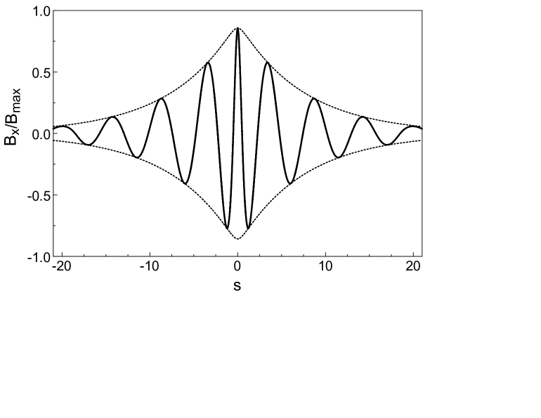
Figure 2: $B_{x}$-component of the soliton solution as a function of dimensionless coordinate $s=K\zeta/2$ in units of $B_{{\rm max}}$ ($B_{{\rm max}}^{2}\equiv 8\pi\rho_{0}C^{2}$): $B_{x}/B_{{\rm max}}=\sqrt{w}\cos\left(\Theta\right)$ shown with the solid line and the amplitude envelope, $\pm\sqrt{w}$ (dashed line). The soliton Mach number $M_{A}=C/C_{A}=3$ corresponds to the amplitude parameter $a=1-M_{A}^{-2}$=8/9.

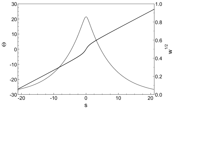
Figure 3: Phase $\Theta$ as a function of coordinate $s$, shown with the solid line. The amplitude of the soliton is shown with the dashed line.

The $B_{x}$-component of the solitary solution is shown in Fig.2 (the $e^{-i\omega t}$ -factor omitted). The wave packet in the compressed area becomes more oscillatory, as may also be seen from Fig.3, which shows the soliton phase $\Theta$ as a function of dimensionless coordinate $s$. The local dimensionless wave number stays approximately constant ($d\Theta/ds\approx 1$), apart from the above phase steepening near the maximum amplitude, where $d\Theta/ds\approx 2$.

4 Maximum Magnetic Field

The isolated solitons obtained in this paper belong to a one parameter family; the amplitude $B_{{\rm max}}$ or Mach number $M_{A}=B_{{\rm max}}/\sqrt{2}B_{0}$ can be used as such parameter. In a CR shock precursor the soliton scale is determined by the scale of seed waves for the subsequent nonresonant instability. The seed waves are resonantly excited upstream of the strong CR current zone by the high energy CRs. Then, $K\sim r_{g}^{-1}(p_{*})$, where $r_{g}$ is the gyroradius of the seed generating CRs of momentum $p=p_{*}$. This amounts to $M_{A}^{2}=k_{J}r_{g}\left(p_{*}\right)$ for the upper (long-wave) soliton branch in eq.(19). Note that $p_{*}$ may be $\ll p_{{\rm max}}$ due to a poor CR confinement in the range $p_{*}<p<p_{{\rm max}}$ (Malkov & Diamond, 2006). If the CR current is sufficiently strong, $k_{J}r_{g}\left(p_{*}\right)\gg 1$ and only the upper-sign soliton in eq.(19) and Fig.1 can accommodate the requirement $K\sim r_{g}^{-1}(p_{*})$ for $M_{A}\gg 1$. Then, the maximum magnetic field for a given soliton can be written as $B_{{\rm max}}^{2}/B_{0}^{2}=2M_{A}^{2}\approx 2k_{J}r_{g}\left(p_{*}\right)$, or

$$B_{{\rm max}}^{2}=4\pi V_{{\rm s}}n_{CR}p_{*},$$ (23)

where $n_{{\rm CR}}$ is the CR density.

The scaling of CR-enhanced magnetic energy with the ambient density $\rho$ and shock velocity $V_{{\rm s}}$ is debated in the literature. Bell (2004) suggested $B^{2}/\rho\propto V_{{\rm s}}^{3}$, whereas Völk et al. (2005) indicate that $B^{2}/\rho\propto V_{{\rm s}}^{2}$. The difference between the two scalings is whether a fraction of mechanical energy flux or momentum flux goes into magnetic energy. By contrast, eq.(23) constitutes the conversion of CR energy flux into magnetic energy. Vink (2008) summarizes the information about the magnetic field from a number of SNR, with the two phenomenological scalings superimposed, Fig.4. Note that $B_{{\rm max}}$ in eq.(23) coincides with the condition of magnetization (trapping by the wave) of the current-carrying particles $k_{J}\left(B_{{\rm max}}\right)r_{g}\left(p_{*},B_{{\rm max}}\right)=1/2$, which is also (formally) similar to the Bell’s phenomenological condition of balancing the Ampere force and the magnetic tension for the instability saturation. However, the saturation mechanism behind eq.(23) is different in that $B_{{\rm max}}$ is only the peak magnetic field. The magnetic energy density would be smaller by a soliton filling factor $f_{{\rm s}}$ (cf. Berezin & Sagdeev, 1969). More importantly, the efficiency of CR acceleration and subsequent conversion of their energy into magnetic field should depend on $J,\;V_{{\rm s}}$ and other acceleration parameters which almost certainly rules out the single power-law relation between $B^{2}/\rho$ and $V_{{\rm s}}$.

Therefore, we obtain such relation in a different way, which we outline below and will describe in detail elsewhere. Consider a nominal SNR with the shock speed $V_{{\rm s}}$ slowing down from an initial $V_{{\rm s}}=V_{0}=1.34\times V_{{\rm ST}}$, to $V_{{\rm{\rm s}}}\approx 0.1\times V_{0}$ (i.e., well into the Sedov-Taylor phase) where $V_{{\rm ST}}=10400\times E_{51}^{1/2}\left(M_{{\rm e}}/M_{\odot}\right)^{1/2}km/s$ (McKee & Truelove, 1995). Here $E_{51}$ is the explosion energy in $10^{51}ergs$ and $M_{{\rm e}}$ -the ejecta mass. During its evolution, the SNR should follow the points sampled from a set of supposedly similar remnants in Fig.4. Using the $V_{{\rm s}}\left(t\right)$ dependence from (McKee & Truelove, 1995), the momentum $p_{*}\sim p_{{\rm max}}\left(t\right)$ in the nonlinear acceleration regime from (Malkov & Drury, 2001, eq.[7.45]), we express $p_{*}$ in eq.(23) as a function of $V_{{\rm s}}$. Next, we obtain $n_{{\rm CR}}$ from eq.(15) in (Malkov, 1997) for the evolving subshock strength with the particle injection rate held approximately constant in the efficient acceleration regime (see eq.(37) in the same reference). Using these results, we finally obtain from eq.(23) an expression for $B_{{\rm max}}^{2}/\rho$, again, as a function of $V_{{\rm s}}$. A preliminary example of such calculation is shown in Fig.4 with the green line. In an intermediate range of $V_{{\rm s}}$ the scaling is $\propto B_{{\rm m}}^{2}/\rho\propto V_{{\rm s}}^{11/4}$ (close to the Bell’s scaling) but it rolls over to turn to zero at $V_{{\rm s}}=V_{0}\approx 9\cdot 10^{4}{\rm km/s}$. This is because the magnetic field generation is pinned to the CRs [eq.(23)] which are not yet there at $V_{{\rm s}}=V_{0}$, i.e. at $t=0$. The other strong deviation from a power-law should occur at lower $V_{{\rm s}}$ where acceleration bifurcates into a inefficient (test particle regime) through a characteristic S-curve.

5 Discussion

The purpose of this paper was to understand the nonlinear evolution of the non-resonant current driven instability by studying saturated nonlinear waves (solitons) as their ensemble (or that of their shock counterparts, if dissipation is efficient) may comprise the asymptotic state of the system. Such scenario is supported by simpler (but fully integrable, e.g., Kaup & Newell, 1978) weakly nonlinear MHD models, such as the derivative nonlinear Schroedinger equation (DNLS, see also Mjolhus & Hada, 1997 for a review). In such models, arbitrary initial conditions evolve into an asymptotic state of quasi-independently propagating solitons, very much similar to those found in the present paper. The difference, however is that our system is driven by the CR return current and its solutions do not transition into the MHD solutions.

The relevant question of soliton stability should be addressed in 2-3D setting. The 2-3D instability of a 1D soliton could comprise a wave front self-focusing (Passot & Sulem, 2003) and thus elucidate the subsequent 3D structures. Such studies are beyond the scope of this letter, but a qualitative stability examination is in order. It may be based on the nonlinear dispersion relation given by eq.(19) and Fig.1. The parts of the dispersion curves with $\partial\left|K\right|/\partial C<0$ (where $K$ and $C\propto M_{A}$ are the wave number and propagation speed) correspond to the solitons with negative dispersion and should be stable. The oft-used justification of stability is that a nonlinear steepening of the soliton’s leading edge generates higher wave number modes and they should not run faster than the soliton itself (negative dispersion is thus required). It should be also noted here that, once the soliton solutions of the driven system are obtained, they can also be arranged in a quasi-periodic or even chaotic soliton lattice. By adding weak dissipation, the leading edges of these solitons can be converted into shock fronts (Sagdeev, 1966) which usually increases the dissipation of the driver energy, thus reducing the saturation amplitude.

To conclude, there exists upper bound on $B_{{\rm max}}$ since solitons with $C/C_{A}=B_{{\rm max}}/\sqrt{2}B_{0}>V_{{\rm s}}/C_{{\rm A}}$ outrun the shock and cannot be sustained by the return current. However, as transients, they may promote particle acceleration far upstream to synergistically supply themselves with the CR return current. This might be a plausible scenario for much-discussed CR acceleration bootstrap (e.g., Malkov & Drury, 2001; Blandford & Funk, 2007). Furthermore, strong solitons running ahead of the shock may become visible in X-rays as quasi-periodic stripes, similar to those recently observed by Chandra (Eriksen et al., 2011) in some parts of the Tycho SNR. The Eriksen’s identification of the stripe spacing with the maximum gyroradius of accelerated particles is consistent with our determination of the soliton spacing in Sec.4, but with a lower than 2 PeV energy. The scale is set by the highest energy particles ahead of the field amplification zone. The soliton wave length should be noticeably shorter than the distance between them. At the same time, similar structures may result from the nonlinear evolution of the CR-pressure-driven acoustic instability studied earlier by Malkov & Diamond (2009). Both the Drury’s (Malkov et al., 2010) and Bells’s instabilities (after adding dissipation to the soliton solution) should result in shock-like nonlinear structures considerably shorter than the conventional CR precursor of the standard Bohm diffusion model. The magnetic field enhancement is clearly weaker in the acoustic case, as it is merely due to the individual shock compression in the instability generated shock-train. Besides, the soliton scenario is exciting as it introduces these fascinating and ubiquitous objects (e.g., Ablowitz & Segur, 1981) to the SNR physics. However, the dominant instability should be selected on a case by case basis by treating the alternatives in a specific shock environment.

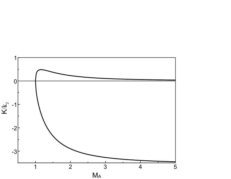
Figure 1: Dispersive properties of the two types of solitons: the short scale (lower branch) and the long scale (upper brunch). The soliton wave number $K$ is shown in the units of $k_{J}=2\pi J/cB_{0}$.

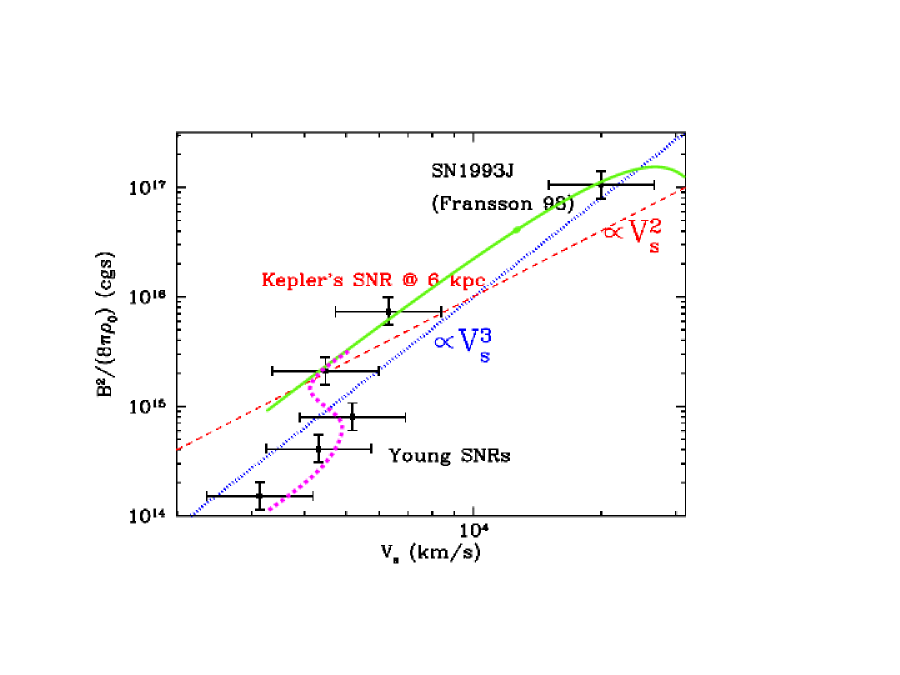
Figure 4: The ratio of magnetic field energy to ambient density $\rho_{0}$ as a function of shock velocity $V_{{\rm s}}$ adopted from (Vink, 2008) (points with error bars). The blue dotted line is the scaling from (Bell, 2004), while the red dashed line is that of (Völk et al., 2005), both also taken from the Vink’s compilation. An example of calculations, described in Sec.4 is shown with the green line. The field energy declines beyond $V_{{\rm s}}\approx 2.7\cdot 10^{4}$ to vanish at $V_{0}\approx 9\cdot 10^{4}{\rm km/s}$ (not shown in the plot). At lower $V_{{\rm s}}$, where the shock acceleration is inefficient, this dependence breaks down and should transition to a low-efficiency acceleration regime in a bistable fashion (Drury & Voelk, 1981; Malkov, 1997) (schematically shown with the magenta dotted line).

References

- Ablowitz & Segur (1981) Ablowitz, M. J., & Segur, H. 1981, Solitons and the inverse scattering transform, ed. Ablowitz, M. J. & Segur, H.
- Achterberg (1983) Achterberg, A. 1983, A&A, 119, 274
- Bell (2004) Bell, A. R. 2004, MNRAS, 353, 550
- Bell (2005) —. 2005, MNRAS, 358, 181
- Berezin & Sagdeev (1969) Berezin, Y. A., & Sagdeev, R. Z. 1969, Soviet Physics Doklady, 14, 62
- Blandford & Funk (2007) Blandford, R., & Funk, S. 2007, in American Institute of Physics Conference Series, Vol. 921, The First GLAST Symposium, ed. S. Ritz, P. Michelson, & C. A. Meegan, 62–64
- Bykov et al. (2009) Bykov, A. M., Osipov, S. M., & Toptygin, I. N. 2009, Astronomy Letters, 35, 555
- Dieckmann et al. (2010) Dieckmann, M. E., Murphy, G. C., Meli, A., & Drury, L. O. C. 2010, A&A, 509, A89+
- Dorfi (1984) Dorfi, E. 1984, Advances in Space Research, 4, 205
- Drury (1984) Drury, L. O. 1984, Advances in Space Research, 4, 185
- Drury & Voelk (1981) Drury, L. O., & Voelk, J. H. 1981, ApJ, 248, 344
- Eriksen et al. (2011) Eriksen, K. A., Hughes, J. P., Badenes, C., Fesen, R., Ghavamian, P., Moffett, D., Plucinksy, P. P., Rakowski, C. E., Reynoso, E. M., & Slane, P. 2011, ApJ, 728, L28+
- Kaup & Newell (1978) Kaup, D. J., & Newell, A. C. 1978, Journal of Mathematical Physics, 19, 798
- Luo & Melrose (2009) Luo, Q., & Melrose, D. 2009, MNRAS, 397, 1402
- Malkov (1997) Malkov, M. A. 1997, ApJ, 491, 584
- Malkov & Diamond (2006) Malkov, M. A., & Diamond, P. H. 2006, ApJ, 642, 244
- Malkov & Diamond (2009) —. 2009, ApJ, 692, 1571
- Malkov et al. (2010) Malkov, M. A., Diamond, P. H., & Sagdeev, R. Z. 2010, Plasma Physics and Controlled Fusion, 52, 124006
- Malkov & Drury (2001) Malkov, M. A., & Drury, L. O. 2001, Reports on Progress in Physics, 64, 429
- McKee & Truelove (1995) McKee, C. F., & Truelove, J. K. 1995, Phys. Rep., 256, 157
- Mjolhus & Hada (1997) Mjolhus, E., & Hada, T. 1997, in Nonlinear Waves and Chaos in Space Plasmas, ed. T. Hada & H. Matsumoto, 121–169
- Niemiec et al. (2008) Niemiec, J., Pohl, M., Stroman, T., & Nishikawa, K.-I. 2008, ApJ, 684, 1174
- Passot & Sulem (2003) Passot, T., & Sulem, P. L. 2003, Physics of Plasmas, 10, 3914
- Pelletier et al. (2006) Pelletier, G., Lemoine, M., & Marcowith, A. 2006, A&A, 453, 181
- Reville et al. (2007) Reville, B., Kirk, J. G., Duffy, P., & O’Sullivan, S. 2007, A&A, 475, 435
- Riquelme & Spitkovsky (2009) Riquelme, M. A., & Spitkovsky, A. 2009, ApJ, 694, 626
- Ryutov et al. (2006) Ryutov, D. D., Furno, I., Intrator, T. P., Abbate, S., & Madziwa-Nussinov, T. 2006, Physics of Plasmas, 13, 032105
- Sagdeev (1966) Sagdeev, R. Z. 1966, Reviews of Plasma Physics, 4, 23
- Sagdeev & Galeev (1969) Sagdeev, R. Z., & Galeev, A. A. 1969, Nonlinear Plasma Theory (W.A. Benjamin Inc. New York, New York)
- Shapiro et al. (1998) Shapiro, V. D., Quest, K. B., & Okolicsanyi, M. 1998, Geophys. Res. Lett., 25, 845
- Stroman et al. (2009) Stroman, T., Pohl, M., & Niemiec, J. 2009, ApJ, 706, 38
- Vink (2008) Vink, J. 2008, in American Institute of Physics Conference Series, Vol. 1085, American Institute of Physics Conference Series, ed. F. A. Aharonian, W. Hofmann, & F. Rieger, 169–180
- Vladimirov et al. (2006) Vladimirov, A., Ellison, D. C., & Bykov, A. 2006, ApJ, 652, 1246
- Völk et al. (2005) Völk, H. J., Berezhko, E. G., & Ksenofontov, L. T. 2005, A&A, 433, 229
- Zirakashvili et al. (2008) Zirakashvili, V. N., Ptuskin, V. S., & Völk, H. J. 2008, ApJ, 678, 255