A $r$-mode in a magnetic rotating spherical layer:
application to neutron stars.

Abstract

The impact of the combination of rotation and magnetic fields on oscillations of stellar fluids is still not well known theoretically. It mixes Alfvén and inertial waves. Neutron stars are a place where both effects may be at work. We wish to decipher the solution of this problem in the context of $r$-modes instability in neutron stars, as it appears when these modes are coupled to gravitational radiation.

We consider a rotating spherical shell filled with a viscous fluid but of infinite electrical conductivity and analyze propagation of modal perturbations when a dipolar magnetic field is bathing the fluid layer. We perform an extensive numerical analysis and find that the $m=2$ $r$-mode oscillation is influenced by the magnetic field when the Lehnert number (ratio of Alfvén speed to rotation speed) exceeds a value proportional to the one-fourth power of the Ekman number (non-dimensional measure of viscosity). This scaling is interpreted as the coincidence of the width of internal shear layers of inertial modes and the wavelength of the Alfvén waves. Applied to the case of rotating magnetic neutron stars, we find that dipolar magnetic fields above $10^{14}$ G are necessary to perturb the $r$-modes instability.

1 Introduction

Numerous astrophysical systems exhibit a pulsating behavior that can be significantly influenced by both magnetic field and rotation. The rapidly oscillating Ap (roAp) stars, the magnetic white dwarf stars and neutron stars as well as planetary cores fall into the above category.

In neutron stars, however, possible astrophysical implications of $r$-modes instability have motivated extensive investigations of this mode during the past few years (see Andersson 2003 for a review). $r$-modes belong to the class of inertial modes that arise in rotating fluids due to the Coriolis force. It was shown by Andersson (1998) and Friedman & Morsink (1998) that these modes easily couple to gravitational radiation and become unstable, allowing the neutron stars to lose their angular momentum.

The foregoing instability may however be weakened or even suppressed by all the dissipative mechanisms which couple to an $r$-mode oscillations. Much work has thus been devoted to the analysis of the various mechanisms which may damp $r$-modes. Recently, vortex-mediated mutual friction of superfluids was investigated by Haskell et al. (2009) as well as the effects of hyperon bulk viscosity Haskell & Andersson (2010), but both effects do not seem to be able to influence the instability at low temperatures. For these temperatures, the Ekman layer which forms below the crust of a neutron star, remains the most important source of dissipation (Bildsten & Ushomirsky 2000; Rieutord 2001; Glampedakis & Andersson 2006).

However, it is well-known that the magnetic field is an important component of a neutron star. It is therefore clear that fluid flows may be seriously influenced by this field and that other channels of dissipation for the $r$-mode instability may exist through this component. Much work was devoted to investigate the modifications induced by a magnetic field on these kind of modes. Rezzolla et al. (2000); Rezzolla et al. (2001a, b), for instance, showed that strong magnetic field, beyond $10^{10}$G may weaken the $r$-mode instability sufficiently so as to make the generated gravitational waves undetectable. Mendell (2001) and Kinney & Mendell (2003) focused their study on the influence of the magnetic field on the Ekman layer flow. They conclude that magnetic field larger than $10^{12}$G completely suppress the instability. However, Lee (2005), using a dipolar magnetic field covering the surface of a neutron star modeled as a $N=1$-polytrope, concludes that much stronger magnetic fields, over $10^{14}$G, are necessary to suppress the instability through magnetic perturbations. Let us note that beside the suppression of the foregoing instability, magnetic fields can also directly spin down a neutron star through the classical process of magnetic braking (i.e. Ho & Lai 2000). More recently, Cuofano & Drago (2010) and Bonanno et al. (2011) investigated the role of magnetic field generation by the unstable $r$-mode, showing that a very strong toroidal magnetic field can be generated, which in turn can modify the instability.

The aim of the present paper is to explore furthermore the channels of dissipation for the unstable $m=2$ $r$-mode of a rotating neutron star, especially when viscosity and magnetic fields are both present. Indeed, a possibility that has not been considered by previous studies (like the one of Lee 2005), is the fact that an unstable $r$-mode of a spherical layer, might develop internal shear layers thanks to the magnetic field action. Since fluid layers of different natures are expected due to phase transitions of nuclear matter, the existence of internal shear layers are also very likely. We shall see that this leads to a threshold value around $10^{14}$G for magnetic fields to noticeably perturb the $r$-mode instability.

Rotating fluid layers bathed by a magnetic field are however not specific to neutron stars. They are also found in planetary core, like in the Earth’s core. Thus, in order to make the following study of more general interest, we shall consider a very simplified model of neutron star, neglecting relativistic or superconducting effects. We thus extend the results of Rieutord (2001) to the case where a dipolar magnetic field perturb the fluid flow (in the limit of very large magnetic Prandtl numbers). This is meant to be a simple configuration where combined effects of magnetic fields and viscosity can be studied.

The paper is organized as follows: In Sect. 2, we recall the basic physical ingredients of the model and then (sect. 3) briefly explain the numerical strategy. Numerical results for the $m=2$ $r$-mode coupled with Alfvén waves are discussed in Sect. 4. Conclusions follow.

2 The model

We consider a rotating star modeled as an infinitely electrically conducting core surrounded by a spherical layer of fluid itself limited by an outer solid crust. The ratio of the inner core radius to the outer radius $R$ is $\eta$. The kinematic viscosity and magnetic diffusivity of the fluid are respectively $\nu$ and $\nu_{m}$.

The star is rotating with uniform angular frequency $\mbox{\boldmath$\Omega$}=\Omega{\bf e}_{z}$ along the z-axis. The core is supposed to be the source of a permanent axisymmetric magnetic dipole covering the whole layer. The symmetry axis of the magnetic field is along the z-axis. Note that such a partition of the star is necessary in order to avoid the problem of the definition of the magnetic field in the core of the star, the dipole field being singular at the center. The fluid in the layer is taken to be incompressible; we thus eliminate phenomena related to compressibility such as $p$-modes (rapid and slow magnetic waves, when a magnetic field is applied). Classical MHD approximations are used (no charge separation, non-relativistic motions, etc.).

2.1 Equations of motion

The shell is bathed by an axisymmetric dipolar magnetic field:

$${\bf B}_{0}=B_{p}\cdot R^{3}\left(\frac{\cos\theta}{r^{3}}{\bf e}_{r}+\frac{\sin\theta}{2r^{3}}\vec{e}_{\theta}\right),$$ (1)

where (${\bf e}_{r},\vec{e}_{\theta},{\bf e}_{\varphi}$) are spherical coordinate unit vectors. $B_{p}$ is the amplitude of the magnetic field at the surface poles of the star.

The equations of motion for an incompressible rotating fluid can be written as

$$\frac{\partial{\bf v}}{\partial t}+{\bf v}\cdot\mbox{\boldmath$\nabla$}{\bf v}+2\mbox{\boldmath$\Omega$}\times{\bf v}=$$

$$-\mbox{\boldmath$\nabla$}p/\rho-\mbox{\boldmath$\nabla$}\Phi_{\rm eff}+\frac{1}{\mu_{0}\rho}({\mbox{\boldmath$\nabla$}}\times{\bf B})\times{\bf B}+\nu\Delta{\bf v},$$ (2a)

$$\frac{\partial{\bf B}}{\partial t}={\mbox{\boldmath$\nabla$}}\times\left({\bf v}\times{\bf B}\right)+\nu_{m}\Delta{\bf B}$$ (2b)

$${\bf\mbox{\boldmath$\nabla$}}\cdot{\bf B}=0,$$ (2c)

$${\bf\mbox{\boldmath$\nabla$}}\cdot{\bf v}=0,$$ (2d)

where $\Phi_{\rm eff}=\Phi-\Omega^{2}r^{2}\sin^{2}\theta/2$ is the effective gravito-rotational potential and $\mu_{0}$ is the permeability of vacuum. Here ${\bf v}$ is the velocity field, ${\bf B}$ is the total magnetic field (dipole field plus perturbation), and $\nu_{m}=1/(\mu_{0}\sigma)$ where $\sigma$ is the fluid’s electrical conductivity.

A non-dimensional form of the previous equations can be obtained by introducing the parameters

$$V_{\rm A}=B_{p}/\sqrt{\mu_{0}\rho},\quad V_{\Omega}=2\Omega R,\quad\mathrm{Le}=V_{\rm A}/V_{\Omega},$$

$$E=\nu/(RV_{\Omega}),\quad E_{m}=\nu_{m}/(RV_{\Omega}),$$

where $V_{\rm A}$ is the Alfvén speed, $V_{\Omega}$ is rotational speed, $E$ is the Ekman number and $E_{m}$ the magnetic Ekman number. Following Jault (2008), we introduce $Le$, the Lehnert number in reference to the work of Lehnert (1954). As shown by its definition, this number measures the ratio of the Alfvén speed to the rotation speed.

By linearizing magneto-hydrodynamic equations (2.1) to the kinetic ${\bf u}$ and magnetic ${\bf b}$ perturbations, one can study infinitesimal perturbations from the equilibrium. We assume these perturbations have a time dependence of the form $\mathrm{e}^{\lambda t}$, where $\lambda=\tau+i\omega$ ($\tau$ is the damping rate, $\omega$ the pulsation and $i^{2}=-1$), and we use the following non-dimensional variables:

$$\begin{array}[]{lll}{\bf v}&\rightarrow&V_{\Omega}{\bf u}({\bf r})e^{\lambda t},\\ {\bf B}&\rightarrow&B_{p}{\bf B}({\bf r})+B_{p}{\bf b}({\bf r})e^{\lambda t},\\ \rho&\rightarrow&\rho_{o},\end{array}$$ (4)

where ${\bf u}({\bf r})$ and ${\bf b}({\bf r})$ are now first order non-dimensional quantities. Therefore, Eqs. (2.1) reduce to the following set of equations:

$$\lambda{\mbox{\boldmath$\nabla$}}\times{\bf u}+{\mbox{\boldmath$\nabla$}}\times({\bf e}_{z}\times{\bf u})=$$

$$\qquad\mathrm{Le}^{2}{\mbox{\boldmath$\nabla$}}\times\left(({\mbox{\boldmath$\nabla$}}\times{\bf b})\times{\bf B}\right)+E{\mbox{\boldmath$\nabla$}}\times\Delta{\bf u},$$ (5a)

$$\lambda{\bf b}={\mbox{\boldmath$\nabla$}}\times\left({\bf u}\times{\bf B}\right)+E_{m}\Delta{\bf b},$$ (5b)

$${\bf\mbox{\boldmath$\nabla$}}\cdot{\bf u}=0,$$ (5c)

$${\bf\mbox{\boldmath$\nabla$}}\cdot{\bf b}=0,$$ (5d)

where ${\bf B}$ denotes the permanent dipolar magnetic field and we used ${\mbox{\boldmath$\nabla$}}\times{\bf B}=0$. Here we take the curl of momentum equation in order to eliminate pressure term.

2.2 Boundary conditions

Six boundary conditions are required in order to solve Eqs. (2.1) uniquely. On the inner boundary $r=\eta R\leavevmode\nobreak\ (\eta<1)$, the magnetic field perturbations have only tangent components because the core is assumed to be infinitely conducting. On the surface $r=R$, the total magnetic field vector matches the external field which is dipolar potential, as there are no currents in the external vacuum. As for the velocity field, we may either use stress-free or no-slip boundary conditions.

As for the magnetic field, different conditions apply for the inner and outer boundaries. On the interior, the perturbation to the electric field is perpendicular to the conducting core, and the perturbation to the magnetic field is tangent. This gives the following three equations:

$$b_{r} = 0,$$ (6a)

$$\displaystyle\frac{E_{m}}{r}\frac{\partial}{\partial r}(rb_{\theta}) = -u_{\theta}B_{r},$$ (6b)

$$\displaystyle\frac{E_{m}}{r}\frac{\partial}{\partial r}(rb_{\varphi}) = -u_{\varphi}B_{r}.$$ (6c)

But actually only (6b) or (6c) together with (6a) is needed (see Reese et al. 2004).

The magnetic field perturbations outside the star ($r>R$) are derived from a potential that does not diverge at infinity:

$${\bf b}_{\rm ext}=\mbox{\boldmath$\nabla$}\phi,$$ (7)

The boundary conditions at the surface of the star are just the continuity of the magnetic field there. These conditions are easily expressed after expansion of the fields in spherical harmonics (see appendix).

Eq. (2.1), together with boundary conditions, defines a generalized eigenvalue problem, where $\lambda$ is the eigenvalue and $({\bf u},{\bf b})$ is the eigenvector which can be computed numerically.

2.3 The case of neutron stars

In neutron stars, typical values for the various physical quantities are

$$B_{p}\sim 10^{12}\leavevmode\nobreak\ {\rm G},\quad\rho\sim 10^{17}\leavevmode\nobreak\ {\rm kg\leavevmode\nobreak\ m}^{-3},\quad R\sim 10\leavevmode\nobreak\ {\rm km},$$ (8a)

$$\Omega=2\pi\nu_{s}\sim 1900\leavevmode\nobreak\ {\rm rad\leavevmode\nobreak\ s}^{-1}$$ (8b)

$$\sigma\sim 5.2\times 10^{17}\leavevmode\nobreak\ {\rm ohm}^{-1}{\rm m}^{-1},\quad\nu\sim 0.32\leavevmode\nobreak\ {\rm m}^{2}{\rm s}^{-1},$$ (8c)

$$\nu_{m}\sim 1.5\times 10^{-12}\leavevmode\nobreak\ {\rm m}^{2}{\rm s}^{-1}.$$ (8d)

Here, the values for $\sigma$ and $\nu$ are given for temperature $T\sim 10^{8}$ K (Baym et al. 1969; Flowers & Itoh 1976, 1979). Therefore, $V_{\rm A}\sim 2.8\times 10^{2}$ m s^-1, $V_{\Omega}\sim 3.8\times 10^{7}$ m s^-1, so that

$$\mathrm{Le}\sim 7.5\times 10^{-6},\quad E\sim 8.4\times 10^{-13},\quad E_{m}\sim 4\times 10^{-24}.$$

We note that the magnetic Prandtl number $\nu/\nu_{m}=E/E_{m}\sim 10^{11}$ is extremely large. This means that the diffusion of magnetic perturbations is a negligible source of dissipation. As a consequence, we may simplify the set of equations (2.1) by setting $E_{m}=0$. In this case the magnetic perturbation is readily given by the fluid flow, namely

$$\lambda\vec{b}={\mbox{\boldmath$\nabla$}}\times(\vec{u}\times\vec{B})$$

Hence, the set of equations reduces to

$$\lambda{\mbox{\boldmath$\nabla$}}\times{\bf u}+{\mbox{\boldmath$\nabla$}}\times({\bf e}_{z}\times{\bf u})=$$

$$\frac{\mathrm{Le}^{2}}{\lambda}{\mbox{\boldmath$\nabla$}}\times\left[({\mbox{\boldmath$\nabla$}}\times{\mbox{\boldmath$\nabla$}}\times(\vec{u}\times\vec{B}))\times{\bf B}\right]+E{\mbox{\boldmath$\nabla$}}\times\Delta{\bf u},$$ (9a)

$${\bf\mbox{\boldmath$\nabla$}}\cdot{\bf u}=0,$$ (9b)

This system is completed by boundary conditions on the velocity solely. Indeed, the magnetic field is completely frozen in the fluid and the magnetic perturbations just represent the oscillations of the dipole field lines. Interestingly, boundary conditions on the magnetic field (6a) show that if $E_{m}=0$ then $u_{\theta}=u_{\varphi}=0$. This means that on the inner core boundary, no slip boundary conditions can be applied. This is expected since the core is assumed at rest and no motion of the field lines is allowed. We also assume no-slip boundary conditions (${\bf u}=\vec{0}$) on the outer boundary to take the crust into account.

The small value of the Lehnert number suggest that the coupling between the $r$-modes and the magnetic field is quite weak. We readily see from the simplified perturbations equations (2.3) that the influence of Lorentz force will be noticeable compared to the viscous one, if $\mathrm{Le}\geq\sqrt{E}$. Noting that the Lorentz operator and the viscous operator are both of second order, we observe that no length scale comes into this inequality. This means that it is valid both in the Ekman boundary layers and in the bulk of the layer. From the numbers that characterize neutron stars it is obvious that the inequality is met. This means that the magnetic field influences the flow more than the viscosity and possibly changes the instability of the $r$-modes. A more detailed calculation is therefore necessary to assess the effect. Actually, we shall see that the previous inequality is not stringent enough and a larger Lehnert number is necessary to affect the instability. We now turn to a numerical study of this problem.

3 Numerical Method

3.1 Spherical harmonic projection

To solve the eigenvalue problem expressed by Eq. (2.1), we project the set of equations on the spherical harmonics in a similar way as in Rieutord (1987, 1991). We expand the perturbed velocity and magnetic fields into poloidal and toroidal components:

$${\bf v}=\sum_{\ell=0}^{\infty}\sum_{m=-\ell}^{\ell}u_{m}^{\ell}(r){\bf R}_{\ell}^{m}+v_{m}^{\ell}(r){\bf S}_{\ell}^{m}+w_{m}^{\ell}(r){\bf T}_{\ell}^{m},$$ (10a)

$${\bf b}=\sum_{\ell=0}^{\infty}\sum_{m=-\ell}^{\ell}a_{m}^{\ell}(r){\bf R}_{\ell}^{m}+b_{m}^{\ell}(r){\bf S}_{\ell}^{m}+c_{m}^{\ell}(r){\bf T}_{\ell}^{m},$$ (10b)

where the radial functions $\{u_{m}^{\ell},v_{m}^{\ell}\}$ ($\{a_{m}^{\ell},b_{m}^{\ell}\}$) and $\{w_{m}^{\ell}\}$ ($\{c_{m}^{\ell}\}$) are the poloidal and toroidal parts of the velocity (magnetic) fields, respectively. ${\bf R}_{\ell}^{m}$, ${\bf S}_{\ell}^{m}$, and ${\bf T}_{\ell}^{m}$ are the vectorial spherical harmonics

$${\bf R}_{\ell}^{m}=Y_{\ell}^{m}{\bf e}_{r},\quad{\bf S}_{\ell}^{m}=r{\bf\nabla}Y_{\ell}^{m},\quad{\bf T}_{\ell}^{m}=r{\mbox{\boldmath$\nabla$}}\times{\bf R}_{\ell}^{m}.$$ (11)

The harmonic decomposition of Eqs. (2.1), (6a) and (7) is given in appendix.

Equation (2.1) reduces to a generalized eigenvalue problem

$${\rm[A]}{\bf x}=\lambda{\rm[B]}{\bf x},$$ (12)

where [A] and [B] are differential operators with respect to the $r$ variable only. The eigenvector associated with $\lambda$ can be written as

$${\bf x}_{\lambda m}(r)=\left|\begin{array}[]{l}\vdots\\ u^{\ell}_{m}(r)\\ c^{\ell}_{m}(r)\\ w^{\ell+1}_{m}(r)\\ a^{\ell+1}_{m}(r)\\ \vdots\\ \end{array}\right.$$ (13)

where $\ell$ is running from $m$ to $\infty$.

3.2 Classification and symmetries

Because of the axisymmetry of background fields, the different $m$’s of the spherical harmonic decomposition are not coupled. An additional simplification comes from the symmetry with respect to equator which permits the separation of symmetric and antisymmetric modes. A more detailed discussion of these points can be found in Reese et al. (2004) in the case of pure Alfvén modes. In the present case, the Coriolis acceleration removes the symmetry $m/-m$, which exists for pure Alfvén modes. Moreover, in the axisymmetric case, poloidal and toroidal components of the fields are coupled.

Figure 1: Top : Absolute value of the damping rate of the $m=2$ $r$-mode as a function of the Lehnert number for various Ekman numbers in $[10^{-7},10^{-4}]$. Bottom: The curves $\tau_{E}(Le)$ are rescaled by the critical Lehnert number. The solid line shows the fit $|\tau|=ax^{4}+bx^{2}+2.45$ with $a=1.67,b=-1.63$. In both panels $\eta=0.35$.

Figure 2: Dependence of the frequency of the $m=2$ $r$-mode as a function of the Lehnert number for various Ekman numbers in $[10^{-6},10^{-4}]$.

Figure 3: The critical Lehnert number as a function of the Ekman number for various aspect ratios $\eta$. The straight line shows the $E^{1/4}$-law.

3.3 Numerical aspects

The numerical resolution of the equations is described in Reese et al. (2004). We just recall here that the equations governing the radial functions $u^{\ell}_{m},v^{\ell}_{m},w^{\ell}_{m},a^{\ell}_{m},b^{\ell}_{m},c^{\ell}_{m}$ are discretized using the Gauss-Lobatto grid and the resulting eigenvalue problem is solved either with a QZ method or with the Arnoldi-Chebyshev algorithm according to whether we solve for the complete spectrum or a few eigenvalues.

4 $r$-modes-Alfvén waves coupling

$r$-modes are a subclass of inertial modes which are purely toroidal. In the case of a non-magnetic and inviscid incompressible fluid, exact analytical solutions exist Rieutord & Valdettaro (1997) and the associated velocity field can be written as

$${\bf u}=\alpha\Omega R(r/R)^{\ell}\bf{T}_{\ell}^{\ell},$$ (14)

where $\alpha$ is an arbitrary constant. The mode’s frequency in the frame corotating with the fluid is given by

$$\omega=-2\Omega/(m+1).$$ (15)

Here, we shall focus on the $m=2$ $r$-mode, which is the most unstable when coupled to gravitational radiation, and track its eigenfrequency and damping rate as the magnetic field is increased.

4.1 The critical Lehnert number

Since we assumed an infinite magnetic Prandtl number, we noted that the boundary conditions on the inner core boundary are of no-slip type. This means that for $\mathrm{Le}\rightarrow 0$ the damping rate follows the law derived in Rieutord (2001), namely

$$\tau=-\frac{35}{2^{7/2}}\frac{1+\eta^{6}}{1-\eta^{7}}{\cal I}_{2}\sqrt{E},\quad{\rm with}\quad{\cal I}_{2}\simeq 0.804$$

If $\eta=0.35$, $\tau=-2.494\sqrt{E}$.

In Fig. 1, we plot the damping rates for various Ekman and Lehnert numbers. The curves show that when the Lehnert number is increased, that is when the magnetic field is increased, the (absolute value of the) damping rate first decreases before rising rapidly. We define a critical Lehnert number, $Le_{c}$, such that $|\tau(Le\geq Le_{c})|\geq|\tau(Le=0)|$. When $\tau$ is plotted as a function of the rescaled Lehnert number, namely $Le/Le_{c}$, all the curves superpose.

For later use, we fit this curve with a simple polynomial in $x=(Le/Le_{c})^{2/3}$, namely $|\tau|=ax^{4}+bx^{2}+2.45$ with $a=1.67,b=-1.63$. The precise shape of the fit is not crucial as long as the values of the minimum and the growth beyond it are respected.

In Fig. 2 we show the variations of the frequency of the $r$-mode with both the Ekman number and the Lehnert number. The curves have been rescaled so as to show a minimized dependence to the parameters. This plot suggests some scaling laws for $\omega-\omega_{0}$, notably that $\omega\simeq\omega_{0}+\omega_{1}\mathrm{Le}^{4}$, $\omega_{1}>0$ for weak magnetic fields. The asymptotic analysis of the behaviour of $\omega$ is quite cumbersome and beyond the scope of this paper.

We show in Fig. 3 that the critical Lehnert number varies quite closely as $E^{1/4}$. Actually, a good fit is $Le_{c}=1.78E^{1/4}$. Magnetic fields will therefore modify the dynamics of the oscillations when $Le\geq Le_{c}$.

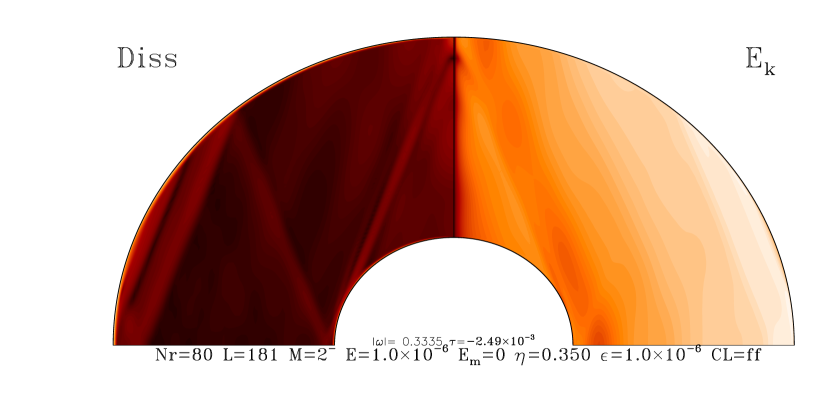
Figure 4: Top : In a meridional plane of the shell, the kinetic energy (right) and viscous dissipation (left) of the m=2 $r$-mode when a weak magnetic field is present (small Lehnert number). Bottom: a view of the associated magnetic perturbation. On right the magnetic energy associated with the oscillation. Left: the associated current. Here E=10^-6, Le=10^-3 and $\eta=0.35$.

The $E^{1/4}$ scaling law of the critical Lehnert number beyond which magnetic field is influential is rather surprising in view of the discussion of sect. 2.3. We may understand this scaling if we consider the nature of $r$-modes when perturbed by a dipolar magnetic field. The magnetic and velocity perturbations, as long as their gradients, are displayed in Fig. 4. It is clear that the magnetic perturbation is concentrated along the shear layer emitted at the critical latitude, namely $\arcsin(1/3)=19.5\textdegree$. Such shear layers are a feature of viscous inertial modes which is due to a singularity of the boundary layer at this latitude (e.g. Rieutord & Valdettaro 2010).

By analyzing the scale of this layer, as shown in appendix, we find that when $Le\gg\sqrt{E}$, its thickness scales like $Le/E^{1/4}$, showing that indeed when $Le$ reaches $E^{1/4}$, the interaction between the magnetic field and the $r$-mode becomes strong, presumably emphasizing a resonance between the oscillating shear layer and an Alfvén wave. From the diminishing of the damping rate, we conclude that the dissipative layers slightly thicken, which is understandable since the magnetic field tends to oppose to shear.

When the Lehnert number is much larger than its critical value the $r$-mode is completely destroyed, leaving the place to small scale (very dissipative) Alfvén waves (see Fig. 5).

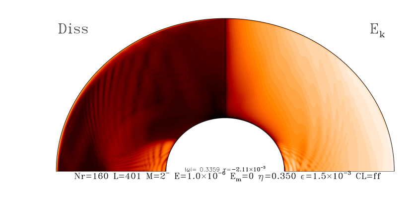
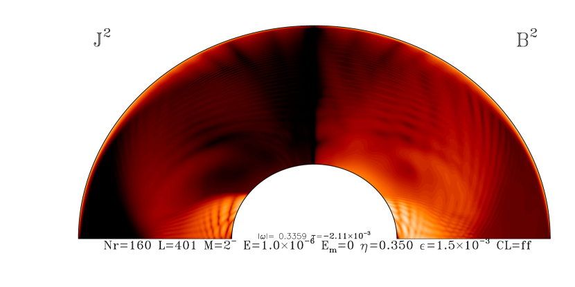
Figure 5: As in figure 4 but with a critical Lehnert number. Note how the dipolar magnetic field now features the various part of the oscillation.

4.2 Influence of the magnetic field on the instability

Let us now turn to the physical consequences of the inequality

$$Le\geq 1.78E^{1/4}.$$

It may be transformed into a constraint on the magnetic field, namely

$$B\geq B_{\rm crit}=1.78\sqrt{\mu_{0}\overline{\rho}}2\Omega RE^{1/4}.$$

We now introduce the scaled angular velocity $\Omega_{*}=\Omega/\sqrt{\pi G\overline{\rho}}$ and the temperature dependence of the kinematic viscosity as in Bildsten & Ushomirsky (2000), namely $\nu=1.8f/T_{8}^{2}$ m²s^-1, where $f$ is a parameter of order unity and $T_{n}=T/10^{n}$. We thus find

$$B_{\rm crit}=7.1\,10^{14}\frac{{\Omega_{*}}^{3/4}}{T_{9}^{1/2}}\;{\rm G}.$$

This critical magnetic field is very high, showing that only hot and slowly rotating neutron stars might be affected by the magnetic field. To visualize this effect, it is useful to consider the window of instability in the plane $(T,\Omega_{*})$ as in Rieutord (2001) or in Bildsten & Ushomirsky (2000).

In order to calculate the boundaries of the window, we need to approximate the curves in Fig. 1 with some analytical function. We thus use the polynomial derived precedingly.

In the plane $(T,\Omega_{*})$, the window boundary gives the critical angular velocity beyond which the $r$-mode instability exists. We therefore need to solve

$$\gamma_{gw}+\gamma_{Bulk}+\gamma_{mi}=0$$

where we take the growth rate of the mode due to gravitational radiation $\gamma_{gw}=0.306\;{\rm s}^{-1}\;\Omega_{*}^{6}$ from Lindblom et al. (1998) and the damping by bulk viscosity $\gamma_{Bulk}=-2.2\,10^{-12}\;{\rm s}^{-1}\;T_{9}^{6}\Omega_{\star}^{2}$ from Lindblom et al. (1999). These expressions of $\gamma_{gw}$ and $\gamma_{Bulk}$ have been derived using an n=1-polytropic model for the neutron star, however we expect that the density distribution influences the damping rate of the mode with a factor of order unity, thus not changing the orders of magnitude of the magnetic fields. We can thus estimate in a simple manner the critical rotation rate for various values of the temperature and magnetic field.

Figure 6: The critical angular velocity, normalized by $\Omega_{K}=\frac{2}{3}\sqrt{\pi G\overline{\rho}}$ for various values of the magnetic field. The solid line shows the case with no magnetic field.

As expected from the value of the critical magnetic field, we see that there is a significant reduction of the instability window only when the field exceeds 10¹⁴ G, which is rather high. However, we note that for lower values (e.g. 10¹³ to 4 10¹³ G), the magnetic field slightly widens the instability window. This is the consequence of the slight reduction of the damping rate around the critical Lehnert number that appears in Fig. 1.

5 Conclusions

In this paper we investigated the dynamics of the $m=2$ $r$-mode in a spherical shell when the fluid is bathed by a dipolar magnetic field. The main theoretical result of this work is that magnetic fields have a negligible influence on the $r$-mode unless they exceed a critical value which is such that the Lehnert number is of the order of the 1/4-power of the Ekman number. A physical interpretation of this scaling law may be obtained by observing that at this critical value, the wavelength of Alfvén waves is similar to R$E^{1/4}$ which is precisely one of the typical thicknesses of shear layers of inertial modes (e.g. Rieutord et al. 2001).

We also have shown that when the magnetic field is slightly below the critical value, the damping rate of the mode is slightly reduced because of the thickening of the various layers due to the frozen field limit.

Back to neutron stars and the famous instability of inertial $r$-modes when coupled to gravitational radiation, we conclude that, as far as dipolar fields are concerned, only fields over $10^{14}$ G may seriously affect the instability. Thus, with a quite different approach, which includes the specific shear layers of $r$-modes, we can confirm the result of Lee (2005), obtained with singular perturbations, that for typical values of $10^{12}$ G, magnetic fields are unimportant.

This result does not therefore invalidate the scenario of Rezzolla et al. (2001b), which suggests that the nonlinear development of the $r$-mode instability may generate a strong toroidal field from a pre-existing poloidal field. This mechanism was recently investigated in some details by Cuofano & Drago (2010) in the context of accreting neutron stars like low-mass X ray binaries. Neglecting viscosity, these authors show that magnetic fields above 10¹² G can reduce the $r$-mode instability. From these results and ours, we estimate that accounting of viscosity will require fields ten times stronger, namely above 10¹³ G. However, the details of the interaction between $r$-modes and a toroidal field in a spherical fluid layer are poorly known: only a few works (e.g. Schmitt 2010, and references therein) have investigated this question in the context of the magnetohydrodynamics of the liquid core of the Earth, where the magnetic Prandtl number is very low. The case relevant to neutron stars still deserves detailed investigations.

The numerical calculations have been carried out on the NEC SX8 of the ‘Institut du Développement et des Ressources en Informatique Scientifique’ (IDRIS) and on the CalMip machine of the ‘Centre Interuniversitaire de Calcul de Toulouse’ (CICT) which are both gratefully acknowledged.

Appendix A spherical harmonic expansion of the MHD equations

In this section , we expand each term of Eq. (2.1) in the spherical harmonics in base of ($R_{\ell}^{m},S_{\ell}^{m},T_{\ell}^{m}$). The different parts of the equation have been published elsewhere: The Lorentz force and the induction equation may be found in Rincon & Rieutord (2003) while the projection of Coriolis acceleration or its curl are in Rieutord (1987); Rieutord & Valdettaro (1997). For completeness we give here the result of casting the projection of these forces into a single equation. The equation of vorticity yields:

$$\lambda w^{l}=\frac{im}{\ell(\ell+1)}w^{l}+A^{l}_{l-1}x^{l-1}\frac{\partial}{\partial x}\biggl{(}\frac{u_{m}^{l-1}}{x^{l-2}}\biggr{)}$$

$$-A^{l}_{l+1}x^{-l-2}\frac{\partial}{\partial x}\biggl{(}x^{l+3}u_{m}^{l+1}\biggr{)}$$

$$+\mathrm{Le}^{2}\left\{\frac{B_{r}}{\ell(\ell+1)r}\left[B^{\ell}_{\ell-1}\partial_{r}(rc^{\ell-1}_{m})\right.\right.$$

$$\left.\left.+B^{\ell}_{\ell+1}\partial_{r}(rc^{\ell+1}_{m})-\frac{im}{\ell(\ell+1)}r\Delta_{\ell}(ra^{\ell}_{m})\right]+\right.$$

$$\left.\frac{B_{\theta}}{r}\left[(\ell+1)\alpha^{\ell}_{\ell-1}c^{\ell-1}_{m}-\ell\alpha^{\ell}_{\ell+1}c^{\ell+1}_{m}\right]\right\}+E\Delta_{\ell}w^{\ell}_{m}$$ (15)

$$\lambda\Delta_{\ell}(ru^{\ell}_{m})-\frac{im}{\ell(\ell+1)}\Delta_{\ell}(ru^{\ell}_{m})+$$

$$B^{\ell}_{\ell-1}r^{\ell-1}\frac{d}{dr}\biggl{(}\frac{w^{\ell-1}_{m}}{r^{\ell-1}}\biggr{)}+B^{\ell}_{\ell+1}r^{-\ell-2}\frac{d}{dr}\biggl{(}r^{\ell+2}w^{\ell+1}_{m}\biggr{)}$$

$$=\mathrm{Le}^{2}\ell(\ell+1)\left\{\frac{B_{\theta}}{r}\left[\ell A^{\ell}_{\ell-1}\Delta_{\ell-1}(ra^{\ell-1}_{m})\right.\right.$$

$$\left.-(\ell+1)A^{\ell}_{\ell+1}\Delta_{\ell+1}(ra^{\ell+1}_{m})+imc^{\ell}_{m}/r\right]$$

$$-B^{\prime}_{\theta}imc^{\ell}_{m}/r$$

$$+B_{r}\left[A^{\ell}_{\ell-1}{\cal D}_{\ell-1}a^{\ell-1}_{m}+A^{\ell}_{\ell+1}{\cal D}_{\ell+1}a^{\ell+1}_{m}\right.$$

$$\left.+\frac{im}{\ell(\ell+1)}\frac{1}{r}\frac{d^{2}rc^{\ell}_{m}}{dr^{2}}\right]$$

$$+B^{\prime}_{r}\left[\frac{}{}A^{\ell}_{\ell-1}\Delta_{\ell-1}(ra^{\ell-1}_{m})+A^{\ell}_{\ell+1}\Delta_{\ell+1}(ra^{\ell+1}_{m})\right.+$$

$$\left.\left.\frac{im}{\ell(\ell+1)}\frac{1}{r}\frac{drc^{\ell}_{m}}{dr}\right]\right\}+E\Delta_{\ell}\Delta_{\ell}(ru^{\ell}_{m})$$ (15)

While the induction equation gives:

$$\lambda ra^{\ell}_{m} = imB_{r}w^{\ell}_{m}+B_{\theta}\left((l+1)\alpha^{\ell}_{\ell-1}u^{\ell-1}_{m}-l\alpha^{\ell}_{\ell+1}u^{\ell+1}_{m}\right)+$$

$$B_{r}\left(B_{l-1}^{l}v^{\ell-1}_{m}+B^{l}_{l+1}v^{\ell+1}_{m}\right)+E_{m}\Delta_{\ell}(ra^{\ell}_{m})$$

$$\lambda c^{\ell}_{m} = \left[\frac{B_{\theta}}{r}\beta^{l}_{k}+\frac{(rB_{r})^{\prime}}{r}\gamma^{\ell}_{k}\right]w^{k}_{m}+B_{r}\gamma^{\ell}_{k}\frac{dw^{k}_{m}}{dr}$$

$$-\frac{im}{\ell(\ell+1)}\left(\ell(\ell+1)B_{\theta}+(rB_{r})^{\prime}\right)\frac{v^{\ell}_{m}}{r}$$

$$-\frac{im}{\ell(\ell+1)}B_{r}\frac{dv^{\ell}_{m}}{dr}+\frac{(rB_{\theta})^{\prime}}{r}\frac{im}{\ell(\ell+1)}u^{\ell}_{m}$$

$$+\frac{im}{\ell(\ell+1)}B_{\theta}\frac{du^{\ell}_{m}}{dr}+E_{m}\Delta_{\ell}c^{\ell}_{m}$$

and the mass and flux conservation read:

$$v_{m}^{\ell}=\frac{1}{\ell(\ell+1)r}\frac{d}{dr}(r^{2}u_{m}^{\ell}),\quad\quad\quad({\bf\mbox{\boldmath$\nabla$}}\cdot{\bf v}=0),$$ (16a)

$$b_{m}^{\ell}=\frac{1}{\ell(\ell+1)r}\frac{d}{dr}(r^{2}a_{m}^{\ell}),\quad\quad\quad({\bf\mbox{\boldmath$\nabla$}}\cdot{\bf b}=0),$$ (16b)

In these equations we introduced the following operators

$$\Delta_{\ell}=\frac{1}{r}\frac{d^{2}}{dr^{2}}r-\frac{\ell(\ell+1)}{r^{2}}$$

$${\cal D}_{\ell}=\frac{1}{r}\frac{d}{dr}r\Delta_{\ell}=\frac{1}{r}\frac{d^{3}}{dr^{3}}r-\frac{\ell(\ell+1)}{r}\frac{d}{dr}\frac{1}{r}$$

and coupling coefficients:

$$\alpha^{l}_{l-1}=\alpha_{l}^{l-1}=\sqrt{\frac{l^{2}-m^{2}}{(2l-1)(2l+1)}}$$

$$\beta^{l}_{l-1}=(l-1)\alpha^{l}_{l-1},\qquad\beta^{l}_{l+1}=-(l+2)\alpha^{l}_{l+1}$$

$$\gamma_{l}^{k}=((k(k+1)+l(l+1)-2)/2k(k+1))\alpha_{l}^{k}$$

$$A^{l}_{l-1}=A_{l}^{l-1}=\alpha^{l}_{l-1}/l^{2}$$

$$B^{l}_{l-1}=B_{l}^{l-1}=(l^{2}-1)\alpha^{l}_{l-1}$$

All the differential equations need to be completed by boundary conditions; for the velocity field, no-slip conditions read:

$$u^{\ell}_{m}=0\qquad\frac{du^{\ell}_{m}}{dr}=0\qquad w^{\ell}_{m}=0$$

on both boundaries. These conditions are sufficient when $E_{m}=0$.

Appendix B Boundary layer analysis for the critical Lehnert number

Let us consider cartesian coordinates adapted to the geometry of the shear layer as shown in Fig. 4 bottom (as materialized by the region with high $\vec{b}^{2}$). $z$ is the coordinate normal to the shear layer assumed to contain the rapid spatial variations.

The dynamics inside this layer verifies

$$\lambda\vec{u}+\omega{\bf e}_{z}\wedge\vec{u}=-\vec{\nabla}p+\frac{Le^{2}}{\lambda}\left({\mbox{\boldmath$\nabla$}}\times\frac{\partial\vec{u}}{\partial z}\right)\times{\bf e}_{z}+E\Delta\vec{u}$$

where we assumed that the background magnetic field is along ${\bf e}_{z}$ and that the shear layer makes an angle $\arcsin\omega$ with the rotation axis (hence the factor $\omega$ in front of Coriolis acceleration). After taking the curl of this equation, considering only the rapid variations along ${\bf e}_{z}$, and taking its $x$ and $y$ components, we find

$$\lambda(\lambda+i\omega)\partial_{z}\overline{u}=(Le^{2}-\lambda E)\partial^{3}_{z}\overline{u}$$

with $\overline{u}=u_{x}+iu_{y}$.

Noting that for $r$-mode $\lambda=-i\omega+\tau_{0}\sqrt{E}$, we find that if $\overline{u}\propto\exp(-z/z_{0})$ then

$$z_{0}\sim(1+i)\frac{Le}{E^{1/4}}$$

This result shows that there is a change of scale in the flow when the Lehnert number reaches values ${\cal O}(E^{1/4})$.

References

- Andersson (1998) Andersson N., 1998, ApJ, 502, 708
- Andersson (2003) Andersson N., 2003, Classical and Quantum Gravity, 20, 105
- Baym et al. (1969) Baym G., Pethick C., Pines D., Ruderman M., 1969, Nature, 224, 872
- Bildsten & Ushomirsky (2000) Bildsten L., Ushomirsky G., 2000, ApJ, 529, L33
- Bonanno et al. (2011) Bonanno L., Cuofano C., Drago A., Pagliara G., Schaffner-Bielich J., 2011, ArXiv e-prints
- Cuofano & Drago (2010) Cuofano C., Drago A., 2010, Phys. Rev. D, 82, 084027
- Flowers & Itoh (1976) Flowers E., Itoh N., 1976, ApJ, 206, 218
- Flowers & Itoh (1979) Flowers E., Itoh N., 1979, ApJ, 230, 847
- Friedman & Morsink (1998) Friedman J. L., Morsink S. M., 1998, ApJ, 502, 714
- Glampedakis & Andersson (2006) Glampedakis K., Andersson N., 2006, MNRAS, 371, 1311
- Haskell & Andersson (2010) Haskell B., Andersson N., 2010, MNRAS, 408, 1897
- Haskell et al. (2009) Haskell B., Andersson N., Passamonti A., 2009, MNRAS, 397, 1464
- Ho & Lai (2000) Ho W. C. G., Lai D., 2000, ApJ, 543, 386
- Jault (2008) Jault D., 2008, Phys. Earth Plan. Int., 166, 67
- Kinney & Mendell (2003) Kinney J. B., Mendell G., 2003, Phys. Rev. D, 67, 024032
- Lee (2005) Lee U., 2005, MNRAS, 357, 97
- Lehnert (1954) Lehnert B., 1954, ApJ, 119, 647
- Lindblom et al. (1999) Lindblom L., Mendell G., Owen B., 1999, Phys. Rev. D, 60, 104014
- Lindblom et al. (1998) Lindblom L., Owen B., Morsink S., 1998, Phys. Rev. Lett., 80, 4843
- Mendell (2001) Mendell G., 2001, Phys. Rev. D, 64, 4009
- Reese et al. (2004) Reese D., Rincon F., Rieutord M., 2004, A&A, 427, 279
- Rezzolla et al. (2001a) Rezzolla L., Lamb F. K., Marković D., Shapiro S. L., 2001a, Phys. Rev. D, 64, 104013
- Rezzolla et al. (2001b) Rezzolla L., Lamb F. K., Marković D., Shapiro S. L., 2001b, Phys. Rev. D, 64, 104014
- Rezzolla et al. (2000) Rezzolla L., Lamb F. K., Shapiro S. L., 2000, ApJ, 531, L139
- Rieutord (1987) Rieutord M., 1987, Geophys. Astrophys. Fluid Dyn., 39, 163
- Rieutord (1991) Rieutord M., 1991, Geophys. Astrophys. Fluid Dyn., 59, 185
- Rieutord (2001) Rieutord M., 2001, ApJ, 550, 443
- Rieutord et al. (2001) Rieutord M., Georgeot B., Valdettaro L., 2001, J. Fluid Mech., 435, 103
- Rieutord & Valdettaro (1997) Rieutord M., Valdettaro L., 1997, J. Fluid Mech., 341, 77
- Rieutord & Valdettaro (2010) Rieutord M., Valdettaro L., 2010, J. Fluid Mech., 643, 363
- Rincon & Rieutord (2003) Rincon F., Rieutord M., 2003, A&A, 398, 663
- Schmitt (2010) Schmitt D., 2010, Geophys. Astrophys. Fluid Dyn., 104, 135