Onset of negative interspike interval correlations in adapting neurons

Abstract

Negative serial correlations in single spike trains are an effective method to reduce the variability of spike counts. One of the factors contributing to the development of negative correlations between successive interspike intervals is the presence of adaptation currents. In this work, based on a hidden Markov model and a proper statistical description of conditional responses, we obtain analytically these correlations in an adequate dynamical neuron model resembling adaptation. We derive the serial correlation coefficients for arbitrary lags, under a small adaptation scenario. In this case, the behavior of correlations is universal and depends on the first-order statistical description of an exponentially driven time-inhomogeneous stochastic process.

I Introduction

Spike-frequency adaptation (SFA) is one of the main adaptation mechanisms in neural systems kandel ; wark2007 . As its name implies, the effect defining SFA is the observation of a scaling in the input-output relationship between the injected current (or a stimulus property) and the firing rate of a spiking neuron, from an initial to a stationary mapping ermentrout1998 ; benda2003 ; higgs2006 ; prescott2008 . Several mechanisms can contribute to SFA (for example, depressing synapses chung2002 ); however, the most prominent mechanism accounting for SFA is the presence of (probably simultaneous) spike-related currents, which produce a negative feedback to the neuron in time scales ranging from tens to thousands of milliseconds benda2003 ; madison1984 ; helmchen1996 ; sah1996 ; hille . Even when the full impact of these currents on neural coding is not completely understood, it is known that they contribute to the processing of static as well as temporal signals. For the processing of temporal signals, it is worth pointing out the high-pass filtering characteristics due to SFA benda2003 ; benda2005 ; benda2010 and its related sensitivity to input fluctuations higgs2006 , the forward masking effect wang1998 ; liu2001 , the selectivity to complex stimuli peron2009a ; peron2009b , and the enhanced reliability of temporal coding prescott2008 .
For the case of static signals, given the absence of a temporal structure in the input, a neural system makes use of a rate code to represent them. A rate code is defined as the number of spikes in a certain temporal window and it is completely described by the spike count statistics dayan . Spike-related adaptation currents have a twofold impact on this code. First, they modify the tuning curve between signals and responses or the input-output relationship mentioned above, which helps to match dynamic ranges wark2007 ; ermentrout1998 ; benda2003 ; higgs2006 ; prescott2008 . Second, they introduce negative correlations between successive interspike intervals (ISIs) in stationary neural spike trains prescott2008 ; benda2010 ; wang1998 ; liu2001 ; avila2011 . While the first effect reflects the modification of the mean spike count, the second effect implies a strong change in its variance (and higher-order properties). This change arises from the fact that the presence of negative correlations in a point process reduces the long-term variability in the counting process that defines the rate code cox . Taken together, both effects deeply affect the encoding reliability avila2011 ; nawrot2007 ; nawrot2010 ; farkhooi2009 ; farkhooi2011 . The presence of negative correlations also affects the coding capabilities of other related schemes; for example, coding of slowly varying signals through a mechanism called noise shaping chacron2004 ; lindner2005 ; avila2009 (demonstrated for negative correlations arising from a history-dependent threshold, but also valid for spike-related adaptation currents), or adaptation-based independent codes nesse2010 .
Correlated single spike trains constitute a nonrenewal point process. In neural systems, this kind of process is relatively ubiquitous lowen ; lowen1992 ; longtin1997 ; ratnam2000 ; chacron2001 (for reviews, mostly based on negative correlations, see also avila2011 ; farkhooi2009 ). In general, there is a coexistence of processes that evoke opposite effects on the ISI correlations, and therefore on the counting statistics in single neurons (adaptation currents and other regularizing processes such as synaptic depression and negative feedback versus filtering and input correlations, among others). Such interesting scenarios have attracted relative attention within the theoretical neuroscience community, and several studies focus on these statistics or related properties in different situations farkhooi2009 ; farkhooi2011 ; lindner2005 ; nesse2010 ; chacron2001 ; middleton2003 ; lindner2004a ; schwalger2008a ; schwalger2010a . Related with our present work, we should note three approaches that have been derived recently: a population-based scheme for adapting ensembles muller2007 (see also farkhooi2009 ; farkhooi2011 ; nesse2010 ), a directed discrete representation for counting events with a general internal structure schwalger2010b (see also lindner2007 ; schwalger2008b ), and a general framework for nonrenewal processes as a hidden Markov model vreeswijk . In particular, our work can be framed within the general approach obtained by van Vreeswijk vreeswijk .
In this work, based on the results we have found in a previous study about the first-passage-time (FPT) problem in an exponentially driven Wiener process urdapilleta , we derive how the resulting negative correlations arise in the spike train of a dynamical, although simple, process resembling the basic features of a spike-related adaptation current added to a spiking neuron in the presence of fast additive fluctuations. The expressions we find are strictly valid in a slight adaptation regime, where the complete FPT density is not necessary and perturbation techniques can be applied, so they remain valid for other dynamical models (with the spike-related adaptation current considered here, or similar). In this way, the onset of correlations due to adaptation is general across different models, provided the additive noise is fast. In the final part of the work, we use the statistics of the FPT problem and the emerging correlations due to adaptation to assess how the spike count variance decreases in comparison to an equivalent neuron without adaptation, in an asymptotic limit. This reduction in the spike count variance underlies the improvement in the decoding performance, and we show how the dependence on the correlations and on the intrinsic variability reduction due to the inhomogeneous driving shape the spike count variance reduction for different spiking frequencies.

II Theoretical framework

II.1 Basic model

We consider an integrate-and-fire (IF) neuron, where subthreshold dynamics of the membrane potential $V$ is governed by

$$C_{\text{m}}\frac{dV}{dt}=f(V)+I_{\text{adapt}}+I_{\text{ext}}.$$ (1)

External, $I_{\text{ext}}$, as well as internal currents, $f(V)$ and $I_{\text{adapt}}$, drive the membrane potential whenever $V<V_{\text{thr}}$. The internal current $f(V)$ takes into account different interspike phenomena, such as leakage or spike initiation onset. The simplest models are the perfect [$f(V)=0$] and the leaky [$f(V)=-g_{L}V$] IF neurons, where only leakage is considered (the perfect IF model corresponds to no leakage). The subthreshold dynamics is supplemented by a threshold condition, which simplifies the highly nonlinear process of a spike excursion: whenever the potential reaches $V_{\text{thr}}$ a spike is defined and immediately, the membrane potential is set to a reset condition $V_{\text{r}}$.
Several types of adaptation currents have been characterized by experiments madison1984 ; helmchen1996 ; sah1996 . According to previous theoretical studies liu2001 ; benda2003 ; benda2010 , we model the adaptation current as a process $x(t)$ that decays during spikes and is incremented when a spike event occurs. In particular, we consider the adaptation current as $I_{\text{adapt}}(t)=-g_{\text{a}}~{}x(t)$, where the interspike dynamics for the adaptation process is given by

$$\frac{dx}{dt}=-\frac{x}{\tau_{\text{a}}},$$ (2)

and a fixed increase $\alpha>0$ is evoked at all spike times $t_{\text{sp}}$: $x(t_{\text{sp}})\rightarrow x(t_{\text{sp}})+\alpha$. This model could be considered as an idealization of the Ca²⁺-dependent K⁺ current, which is widely expressed in neurons exhibiting SFA [$x(t)$ would represent the calcium concentration in a current-based scheme]. Without mathematical loss, we can set $g_{\text{a}}=C_{\text{m}}/\tau_{\text{a}}$ and use $\alpha$ to control the strength of the adaptation current.
Since $I_{\text{adapt}}(t)=-(C_{\text{m}}/\tau_{\text{a}})~{}x(t)$, from Eq. (2) it follows that, between the ($n$)th and the ($n+1$)th spikes, the evolution of the adaptation current is given by

$$\frac{I_{\text{adapt}}(t)}{C_{\text{m}}}=-\frac{\varepsilon_{\text{n}}}{\tau_{\text{a}}}~{}\exp[-(t-t_{\text{n}})/\tau_{\text{a}}],$$ (3)

where $\varepsilon_{\text{n}}$ represents the state of the adaptation process $x$ immediately after the spike time $t_{\text{n}}$.
Without a random component, the deterministic dynamics of the membrane potential in the IF model with an adaptation current, Eqs. (1) and (3), evolves along a prescribed trajectory and no correlations emerge since each ISI is a replica of itself (however, even in the deterministic regime, perturbations propagate in the sequence of ISIs, which induces correlations schwalger2010a ). We introduce a stochastic component in the system through external noise. In particular, we assume that the external current is given by a constant deterministic component and an additive Gaussian white noise representing fast external fluctuations

$$\frac{I_{\text{ext}}}{C_{\text{m}}}=\mu+\xi(t),$$ (4)

where $\langle\xi(t)\rangle=0$ and $\langle\xi(t)\xi(t^{\prime})\rangle=2D\delta(t^{\prime}-t)$. Therefore, the subthreshold dynamics between the ($n$)th and the ($n+1$)th spikes is determined by

$$\frac{dV}{dt}=g(V)+\mu-\frac{\varepsilon_{\text{n}}}{\tau_{\text{a}}}~{}\exp[-(t-t_{\text{n}})/\tau_{\text{a}}]+\xi(t).$$ (5)

Different (IF) models will have different $g(V)$ functions. In particular, $g(V)=0$ for the perfect IF model and $g(V)=-V/\tau_{\text{m}}$, with $\tau_{\text{m}}=C_{\text{m}}/g_{L}$, for the leaky IF model. The threshold condition (at spike time $t_{\text{n}+1}$) resets the membrane potential to $V_{\text{r}}$ and updates the adaptation state to $\varepsilon_{\text{n+1}}=\varepsilon_{\text{n}}~{}\exp(-\tau_{\text{n}}/\tau_{\text{a}})+\alpha$, where $\tau_{\text{n}}=t_{\text{n}+1}-t_{\text{n}}$ is the ($n$)th ISI.
In Fig. 1(a) we show a typical realization of the membrane potential, $V(t)$, and the adaptation process, $x(t)$, for the system described above. As shown in Fig. 1(b), this model exhibits SFA, where a step input (bottom) induces an initial firing rate $f_{\text{0}}$ which decays to a lower steady-state firing rate $f_{\text{ss}}$ (top), with some typical time scale. Spike times $t_{\text{n}}$ defining the spike train, $T_{\text{sp}}(t)=\sum\delta(t-t_{\text{n}})$ [see top of Fig. 1(a)], also establish the sequence of FPT processes, $\{\dots,\tau_{\text{n-1}},\tau_{\text{n}},\tau_{\text{n+1}},\dots\}\equiv\{\tau_{\text{n}}\}$ [Fig. 1(c)]. The ongoing (initial) state of the adaptation process, $\varepsilon_{\text{n}}$, is a history-dependent random variable turning the sequence $\{\tau_{\text{n}}\}$ into non-Markovian.

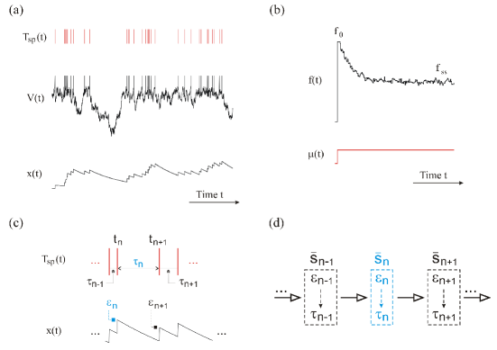
Figure 1: (Color online) Neuron model with adaptation current. (a) A system realization, $V(t)$ and $x(t)$, and the resulting spike train $T_{\text{sp}}(t)$. (b) The system develops spike-frequency adaptation (top), usually characterized by the temporal evolution of the firing frequency, $f(t)$, stimulated with step currents (bottom). (c) A sample trace of the adaptation process $x(t)$ and the basic elements used to describe the stochastic nature of the system, $\varepsilon$ and $\tau$. (d) The hidden Markov model, composed by $\varepsilon$ and the observable $\tau$, used for the analysis.

However, the bidimensional state $\overline{s}=(\varepsilon,\tau)$, defined at spike times, supports a Markovian process since the state at (spike) time $t_{\text{n}}$ is completely characterized from the knowledge of the state at (spike) time $t_{\text{n-1}}$: given $\varepsilon_{\text{n-1}}$ and $\tau_{\text{n-1}}$, $\varepsilon_{\text{n}}$ is defined by the deterministic relationship $\varepsilon_{\text{n}}=\varepsilon_{\text{n-1}}~{}\exp(-\tau_{\text{n-1}}/\tau_{\text{a}})+\alpha$, and $\tau_{\text{n}}$ is given by the FPT problem of a certain stochastic process with an exponential time-dependent drift $(-\varepsilon_{\text{n}}/\tau_{\text{a}})\exp[-(t-t_{\text{n}})/\tau_{\text{a}}]$. In particular, for the perfect (leaky) IF model, the underlying stochastic process is a Wiener (Ornstein-Uhlenbeck) diffusion process. In mathematical terms, the transition probability density is given by

$$f(\overline{s}_{\text{n}}|\overline{s}_{\text{n-1}},\overline{s}_{\text{n-2}},\dots)\hskip 113.81102pt$$

$$=f(\varepsilon_{\text{n}},\tau_{\text{n}}|\varepsilon_{\text{n-1}},\tau_{\text{n-1}})\hskip 103.85237pt$$

$$=\delta\{\varepsilon_{\text{n}}-[\varepsilon_{\text{n-1}}\exp(-\tau_{\text{n-1}}/\tau_{\text{a}})+\alpha]\}~{}\phi(\tau_{\text{n}}|\varepsilon_{\text{n}}),$$ (6)

where $\phi(\tau_{\text{n}}|\varepsilon_{\text{n}})$ is the FPT density function associated to the ($n$)th ISI, which depends exclusively on $\varepsilon_{\text{n}}$ and not on previous outcomes ($t_{\text{n}}$ in the above notation for the drift just set the initial time). This Markovian process is represented in Fig. 1(d) and constitutes a hidden Markov model. Based on Eq. (II.1), the key elements necessary to analyze this stochastic system are the statistics of $\varepsilon$ and the time-inhomogeneous FPT density function.

II.2 Statistics of the (initial) adaptation strength

For one-dimensional systems as the IF models, the solution to the FPT problem is given as an expansion in terms of the strength of the exponential drift urdapilleta ; comment1

$$\phi(\tau|\varepsilon)=\sum_{\text{i}=0}^{\infty}\varepsilon^{\text{i}}~{}\phi_{\text{i}}(\tau).$$ (7)

Given the transition density, Eq. (II.1), the equilibrium probability density for $\varepsilon$, $\rho_{\text{eq}}(\varepsilon)$, should satisfy vreeswijk

$$\rho_{\text{eq}}(\varepsilon_{\text{n}})=\int f_{\varepsilon}(\varepsilon_{\text{n}}|\varepsilon_{\text{n-1}})~{}\rho_{\text{eq}}(\varepsilon_{\text{n-1}})~{}d\varepsilon_{\text{n-1}},$$ (8)

where the transition density between substates is

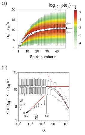
Figure 2: (Color online) Statistics of $\varepsilon$ for the perfect IF model. (a) Density of normalized $\varepsilon$ as a function of the spike number (color bar in logarithmic scale). Symbols and error bars indicate mean and standard deviation, respectively. The analytical expression for the mean as a function of the spike number, Eq. (16), is represented by the dotted (blue) line. The analytical expressions for the stationary properties (mean/standard deviation), Eqs. (11) and (12), are indicated by arrows at the right (black/gray). Numerical results were obtained for $\mu=0.10~{}\text{ms}^{-1}$, $D=0.05~{}\text{ms}^{-1}$, $V_{\text{thr}}-V_{\text{r}}=1.0$, $\tau_{\text{a}}=100.0~{}\text{ms}$, and $\alpha=0.01$ (number of trials, $N_{\text{trials}}=10^{5}$). (b) The normalized stationary mean as a function of $\alpha$ (semilogarithmic plot). The analytical result is represented by a continuous (red) line. Nonlinear effects for large $\alpha$ are fitted by a (dashed-dotted) line, indicating that linear regime remains valid up to $\alpha\approx 0.1$. Inset: plot of the (not normalized) stationary mean as a function of $\alpha$. Same parameters as in (a), except that $N_{\text{trials}}=10^{3}$ for each point.

$$f_{\varepsilon}(\varepsilon_{\text{n}}|\varepsilon_{\text{n}-1})=\int f(\varepsilon_{\text{n}},\tau_{\text{n}}|\varepsilon_{\text{n-1}},\tau_{\text{n-1}})\phi(\tau_{\text{n-1}}|\varepsilon_{\text{n-1}})d\tau_{\text{n}}d\tau_{\text{n-1}}.$$ (9)

Replacing Eq. (II.1) and the $\varepsilon$-expansion for $\phi(\tau_{\text{n-1}}|\varepsilon_{\text{n-1}})$, Eq. (7), in Eq. (9) we obtain a self-consistent integral equation, hard to tackle analytically. However, from this integral equation it is relatively simple to find a relationship between the moments, which reads

$$\langle\varepsilon_{\text{n}}^{\text{m}}\rangle = \int\varepsilon_{\text{n}}^{\text{m}}~{}\rho_{\text{eq}}(\varepsilon_{\text{n}})~{}d\varepsilon_{\text{n}}$$ (10)

$$= \alpha^{\text{m}}+\sum_{\text{i}=1}^{\text{m}}\binom{\text{m}}{\text{i}}~{}\alpha^{\text{m}-\text{i}}~{}\sum_{\text{j}=0}^{\infty}\phi_{\text{j}}^{L}(\text{i}/\tau_{\text{a}})~{}\langle\varepsilon_{\text{n-1}}^{\text{i}+\text{j}}\rangle,$$

where $\binom{a}{b}$ is the binomial coefficient and $\phi_{\text{j}}^{L}(s)$ is the Laplace transform of the $j$th term in the expansion for the FPT solution. The previous relationship relates unconditional moments (subindexes are irrelevant), and therefore it represents a set of infinite algebraic equations for the (infinite) moments $\langle\varepsilon^{\text{m}}\rangle$.
In the slight adaptation regime, $\alpha\neq 0$ but small, it is easy to see that the moments $\langle\varepsilon^{\text{m}}\rangle\sim\mathcal{O}(\alpha^{\text{m}})$. In particular, the first two moments read

$$\langle\varepsilon\rangle = \frac{\alpha}{[1-\phi_{0}^{L}(1/\tau_{\text{a}})]},$$ (11)

$$\langle\varepsilon^{2}\rangle = \frac{\alpha^{2}~{}[1+\phi_{0}^{L}(1/\tau_{\text{a}})]}{[1-\phi_{0}^{L}(1/\tau_{\text{a}})]~{}[1-\phi_{0}^{L}(2/\tau_{\text{a}})]}.$$ (12)

The $\alpha$-normalized properties, $(1/\alpha)\langle\varepsilon\rangle$ and $(1/\alpha^{2})\langle(\varepsilon-\langle\varepsilon\rangle)^{2}\rangle$, are shown in Fig. 2(a) in black and gray arrows, respectively (right margin), for the case of the perfect IF neuron model. As expected, they agree with the results obtained from simulations in the asymptotic limit (symbols plus error bars: mean plus standard deviation of $\varepsilon_{\text{n}}$; colored histogram: logarithm of the density).
For small $\alpha$ values, there is an additional interesting viewpoint to derive $\langle\varepsilon\rangle$, also valid for any neuron model. Multitrial experiments usually start from rest, where we assume that there is no adaptation, $\varepsilon_{0}=0$. Conditional to this fact, the ($n$)th event satisfies

$$\varepsilon_{\text{n}}=\alpha~{}[1+\sum_{\text{i}=1}^{\text{n}-1}\prod_{\text{j}=\text{i}}^{\text{n}-1}\exp(-\tau_{\text{j}}/\tau_{\text{a}})].$$ (13)

The first moment is given by

$$\langle\varepsilon_{\text{n}}\rangle=\alpha~{}[1+\sum_{\text{i}=1}^{\text{n}-1}\langle\prod_{\text{j}=\text{i}}^{\text{n}-1}\exp(-\tau_{\text{j}}/\tau_{\text{a}})\rangle].$$ (14)

For a weak adaptation process we consider that $\langle\epsilon_{\text{n}}\rangle\sim\mathcal{O}(\alpha)$, and then the conditional probabilities required in the above expression are well approximated by their zero-order expansion, $f_{\tau}(\tau_{\text{n}}/\tau_{\text{n-1}},\tau_{\text{n-2}},\dots)=\phi_{0}(\tau_{\text{n}})$ for all $n$. In this limit it is easy to see that

$$\langle\varepsilon_{\text{n}}\rangle = \alpha~{}[1+\sum_{\text{i=1}}^{\text{n}-1}\prod_{\text{j}=\text{i}}^{\text{n}-1}\langle\exp(-\tau_{\text{j}}/\tau_{\text{a}})\rangle_{\phi_{0}}]$$ (15)

$$= \alpha~{}\sum_{\text{i}=0}^{\text{n}-1}[\phi_{0}^{L}(1/\tau_{\text{a}})]^{\text{i}},$$

where $\langle\cdot\rangle_{\phi_{\text{i}}}$ indicates the average with respect to the function $\phi_{\text{i}}(\tau)$. This geometric series is readily obtained:

$$\langle\varepsilon_{\text{n}}\rangle=\alpha~{}\frac{1-[\phi_{0}^{L}(1/\tau_{\text{a}})]^{\text{n}}}{[1-\phi_{0}^{L}(1/\tau_{\text{a}})]},$$ (16)

and converges asymptotically to $\alpha/[1-\phi_{0}^{L}(1/\tau_{\text{a}})]$, whenever $\phi_{0}^{L}(1/\tau_{\text{a}})<1$, in concordance with the previous analysis. The exponential growth of the normalized adaptation strength $(1/\alpha)\langle\varepsilon_{\text{n}}\rangle$, predicted by Eq. (16), is shown in Fig. 2(a) as a function of the spike number $n$ (blue dotted line), together with the results obtained from numerical simulations (symbols). The agreement is remarkable for this case (simulation results were obtained with $\alpha=0.01$).
In order to determine the range of $\alpha$ where the approximation remains valid, we run several simulations and calculate the asymptotic (equilibrium) $\langle\varepsilon\rangle$ for different $\alpha$ values. In Fig. 2(b) we show the normalized asymptotic mean value as a function of $\alpha$ (inset: not normalized mean value). The average exhibits the linear behavior indicated by the preceding results up to $\alpha\approx 0.1$, which represents an adaptation of about $10\%$ [$(f_{0}-f_{\text{ss}})/f_{0}$, see Fig. 1(c)].

III Results

III.1 Onset of correlations

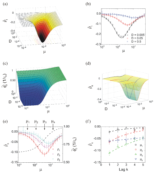
Figure 3: (Color online) Normalized serial correlation coefficients (SCC), $\hat{\rho}_{k}=\rho_{k}/\alpha$, for the perfect IF model. (a) Theoretical expression for the normalized first SCC as a function of driving parameters, $\mu$ and $D$ ($\text{ms}^{-1}$) [see Eq. (III.1)]. (b) Numerical results (symbols) for the normalized first SCC as a function of $\mu$ ($\text{ms}^{-1}$) and different $D$ values ($\text{ms}^{-1}$). Corresponding theoretical expressions are indicated by continuous lines. (c) Factor $\phi_{0}^{L}(1/\tau_{\text{a}})$, which defines the relationship between successive SCC values, as a function of the driving parameters. (d) Theoretical prediction of normalized SCC at higher lags as a function of driving parameters [see Eq. (26)]. Continuous, dashed, and dashed-dotted (colored) lines represent $\hat{\rho}_{1}$, $\hat{\rho}_{2}$, and $\hat{\rho}_{3}$, respectively, at different noise intensities (black, red, blue, and orange: $D=10^{0}$, $10^{-2}$, $10^{-4}$, and $10^{-6}~{}\text{ms}^{-1}$, respectively). Lines are embedded in their respective continuous (semitransparent) surfaces. (e) Numerical results for the normalized SCC at higher lags. $\hat{\rho}_{1}$, $\hat{\rho}_{3}$, and $\hat{\rho}_{5}$ as a function of $\mu$ ($\text{ms}^{-1}$, $D=0.05~{}\text{ms}^{-1}$). Continuous lines represent the corresponding theoretical expressions. Dashed black line indicates $\phi_{0}^{L}(1/\tau_{\text{a}})$ (right scale). (f) Numerical results for the normalized SCC as a function of the lag for the four cases indicated with arrows in (e). Dashed lines indicate theoretical expressions. Ratios between successive SCCs are given by the value of $\phi_{0}^{L}(1/\tau_{\text{a}})$ at each point [dashed line in (e) at the different values of $\mu$]. Numerical results were obtained from $N_{\text{ISI}}=10^{6}$ consecutive ISIs, error bars were estimated from $N_{\text{repet}}=10$ repetitions. Remaining parameters: $V_{\text{thr}}-V_{\text{r}}=1.0$, $\tau_{\text{a}}=100.0~{}\text{ms}$, and $\alpha=0.1$.

Correlations in nonrenewal point processes are usually characterized by the serial correlation coefficient (SCC), which is defined by

$$\rho_{\text{k}}=\frac{\langle\tau_{\text{n}}\tau_{\text{n}+\text{k}}\rangle-\langle\tau_{\text{n}}\rangle\langle\tau_{\text{n}+\text{k}}\rangle}{\sqrt{\langle\Delta\tau_{\text{n}}^{2}\rangle\langle\Delta\tau_{\text{n}+\text{k}}^{2}\rangle}},$$ (17)

where $k$ indicates the lag between successive ISIs, brackets indicate ensemble average, and $\Delta\tau_{\text{i}}^{2}=(\tau_{\text{i}}-\langle\tau_{\text{i}}\rangle)^{2}$ is the variance. Once the system reaches the stationary conditions (the firing frequency is adapted), the SCC simplifies to

$$\rho_{\text{k}}=\frac{\langle\tau_{\text{n}}\tau_{\text{n}+\text{k}}\rangle-\langle\tau\rangle^{2}}{\langle\Delta\tau^{2}\rangle}.$$ (18)

For the hidden Markov model defined by Eq. (II.1), $\langle\tau_{\text{n}}\tau_{\text{n}+\text{k}}\rangle$ reads

$$\langle\tau_{\text{n}}\tau_{\text{n}+\text{k}}\rangle=\int_{\mathcal{D}s_{\text{n}}}\int_{\mathcal{D}s_{\text{n}+\text{k}}}\tau_{\text{n}}\tau_{\text{n}+\text{k}}~{}f(\varepsilon_{\text{n}+\text{k}},\tau_{\text{n}+\text{k}}|\varepsilon_{\text{n}},\tau_{\text{n}})$$

$$\times~{}\phi(\tau_{\text{n}}|\varepsilon_{\text{n}})~{}\rho_{\text{eq}}(\varepsilon_{\text{n}})~{}ds_{\text{n}}~{}ds_{\text{n}+\text{k}},$$ (19)

where $ds_{\text{i}}$ represents $d\varepsilon_{\text{i}}d\tau_{\text{i}}$ and $\mathcal{D}s_{\text{i}}$ its integration domain.
At lag $\text{k}=1$, the transition probability density between states is given directly by Eq. (II.1). The onset of correlations is characterized by the smallest order in $\alpha$ which produce finite SCC values. This order coincides with the small adaptation regime, and therefore, the linear $\varepsilon$-expansion suffices for relevant expressions in Eq. (III.1), $\langle\tau_{\text{n}}\tau_{\text{n}+1}\rangle\sim\mathcal{O}(\alpha)$. Consequently, we obtain

$$\langle\tau_{\text{n}}\tau_{\text{n}+1}\rangle=\langle\tau\rangle_{\phi_{0}}^{2}\hskip 149.37697pt$$

$$+~{}\alpha~{}\langle\tau\rangle_{\phi_{1}}\left[\frac{\langle\varepsilon\rangle}{\alpha}\left(\langle\tau\rangle_{\phi_{0}}-\frac{d\phi_{0}^{L}(s)}{ds}\rfloor_{1/\tau_{\text{a}}}\right)+\langle\tau\rangle_{\phi_{0}}\right],$$ (20)

where $\langle\cdot\rangle_{\phi_{\text{i}}}$ indicates the average with respect to the function $\phi_{\text{i}}(\tau)$. In order to keep the linear order in the normalization required for the SCC, we have $\langle\tau\rangle^{2}\sim\mathcal{O}(\alpha)$ and $\langle\Delta\tau^{2}\rangle\sim\mathcal{O}(0)$:

$$\langle\tau\rangle^{2} = \langle\tau\rangle_{\phi_{0}}^{2}+2\langle\varepsilon\rangle\langle\tau\rangle_{\phi_{0}}\langle\tau\rangle_{\phi_{1}},$$ (21)

$$\langle\Delta\tau^{2}\rangle = \langle\Delta\tau^{2}\rangle_{\phi_{0}}.$$ (22)

In Eqs. (III.1) and (21), the evaluation of $\langle\varepsilon\rangle$ should be performed in the linear regime. Taking into account the results obtained in the previous section, $\langle\varepsilon\rangle/\alpha=1/[1-\phi_{0}^{L}(1/\tau_{\text{a}})]$, the first SCC reads

$$\rho_{1}=-\alpha~{}\frac{\langle\tau\rangle_{\phi_{1}}}{[1-\phi_{0}^{L}(1/\tau_{\text{a}})]~{}\langle\Delta\tau^{2}\rangle_{\phi_{0}}}~{}\hskip 56.9055pt$$

$$\times~{}\left[\phi_{0}^{L}(1/\tau_{\text{a}})\langle\tau\rangle_{\phi_{0}}+\frac{d\phi_{0}^{L}(s)}{ds}\rfloor_{1/\tau_{\text{a}}}\right].$$ (23)

To evaluate the SCC at higher lags, $\text{k}>1$, we need to obtain the transition probability density between the states $n$ and $n+k$ which, based on the hidden Markov model, reads

$$\begin{split}f(\varepsilon_{\text{n}+\text{k}},\tau_{\text{n}+\text{k}}|\varepsilon_{\text{n}},\tau_{\text{n}})&=&\dotsint_{\mathcal{D}s^{(\text{k}-1})}ds^{(\text{k}-1)}~{}f(\varepsilon_{\text{n}+\text{k}},\tau_{\text{n}+\text{k}},\dots,\varepsilon_{\text{n}+1},\tau_{\text{n}+1}|\varepsilon_{\text{n}},\tau_{\text{n}})\\ &=&\dotsint_{\mathcal{D}s^{(\text{k}-1})}ds^{(\text{k}-1)}\prod_{\text{i}=1}^{\text{k}}f(\varepsilon_{\text{n}+\text{i}},\tau_{\text{n}+\text{i}}|\varepsilon_{\text{n}+\text{i}-1},\tau_{\text{n}+\text{i}-1}),\end{split}$$ (24)

where we have simplified the notation to $ds^{(\text{k}-1)}=ds_{\text{n}+1}\dots ds_{\text{n}+\text{k}-1}$ and $\mathcal{D}s^{(\text{k}-1)}$ to the corresponding integration domain. Each of the factors under the product symbol has the structure given by Eq. (II.1). After some calculus [it is convenient to leave unevaluated all integrals in $\tau_{\text{i}}$ in the transition density from $\overline{s}_{\text{n}}$ to $\overline{s}_{\text{n}+\text{k}}$, for posterior evaluation in Eq. (III.1)], the average between successive ISIs is given, up to first order in $\alpha$ (and/or $\langle\varepsilon\rangle$), by

$$\langle\tau_{\text{n}}\tau_{\text{n}+\text{k}}\rangle=\langle\tau\rangle_{\phi_{0}}^{2}~{}+~{}\alpha~{}\langle\tau\rangle_{\phi_{1}}\hskip 99.58464pt$$

$$\times\Bigg{[}\Big{(}1+\frac{\langle\varepsilon\rangle}{\alpha}\Big{)}\langle\tau\rangle_{\phi_{0}}+\langle\tau\rangle_{\phi_{0}}\sum_{\text{i}=1}^{\text{k}-1}[\phi_{0}^{L}(1/\tau_{\text{a}})]^{\text{k}-\text{i}}$$

$$-\frac{\langle\varepsilon\rangle}{\alpha}[\phi_{0}^{L}(1/\tau_{\text{a}})]^{\text{k}-1}\frac{d\phi_{0}^{L}(s)}{ds}\rfloor_{1/\tau_{\text{a}}}\Bigg{]}.$$ (25)

Replacing the stationary value for $\langle\varepsilon\rangle$, and after normalization, it is relatively simple to prove that SCC values at superior lags are given by

$$\rho_{\text{k}}=[\phi_{0}^{L}(1/\tau_{\text{a}})]^{\text{k}-1}~{}\rho_{1}~{},\hskip 28.45274pt\text{k}>1.$$ (26)

For the perfect IF model, the lowest orders in the expansion corresponding to the solution of the FPT problem, Eq. (7), are given urdapilleta , and therefore, the expressions for $\rho_{\text{k}}$ can be explicitly evaluated.
In Fig. 3(a) we show the normalized first SCC, $\hat{\rho}_{1}=\rho_{1}/\alpha$, as a function of the parameters governing the dynamics of the perfect IF neuron model, $\mu$ and $D$. In Fig. 3(b) we show the theoretical expression for the normalized SCC $\hat{\rho}_{1}$ as a function of the driving force $\mu$, for different noise intensities, and compare it with numerical results. The agreement between both curves is remarkable, since the limit of small adaptation is satisfied (numerical results were obtained with $\alpha=0.1$ and then normalized).

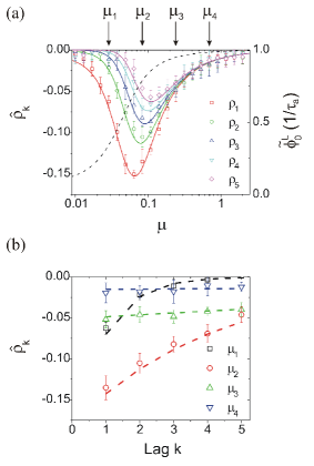
Figure 4: (Color online) Normalized serial correlation coefficients (SCCs), $\hat{\rho}_{\text{k}}=\rho_{\text{k}}/\alpha$, for the leaky IF model [$g(V)=-V/\tau_{\text{m}}$]. (a) and (b) analogous to Figs. 3(e) and  3(f). Parameters: $\tau_{\text{m}}=10.0~{}\text{ms}$, $D=0.01~{}\text{ms}^{-1}$, $V_{\text{thr}}-V_{\text{r}}=1.0$, and $\tau_{\text{a}}=100.0~{}\text{ms}$.

As expressed by Eq. (26), the SCC at higher lags, $\rho_{\text{k}}$ for $k>1$, have a geometric structure: $\rho_{\text{k}}=\phi_{0}^{L}(1/\tau_{\text{a}})~{}\rho_{\text{k}-1}$. Since $0<\phi_{0}^{L}(1/\tau_{\text{a}})<1$ [see Fig. 3(c)], SCC at higher lags are scaled versions of the first SCC. In Fig. 3(d) we show the first three normalized SCC, $\hat{\rho}_{\text{k}}=\rho_{\text{k}}/\alpha$, as a function of the parameters $\mu$ and $D$. As stated by the geometric relationship, the exact scaling between them is given according to the precise location in the parameters space [equivalent point in Fig. 3(c)]. The scaling can be better appreciated in Fig. 3(e), which simply represents a section of Fig. 3(d) along a particular $D$. In this case, theoretical (solid lines) as well as numerical results (symbols) for $\hat{\rho_{1}}$, $\hat{\rho_{3}}$, and $\hat{\rho_{5}}$ are represented as a function of the driving force $\mu$ ($\hat{\rho}_{2}$ and $\hat{\rho}_{4}$ are omitted for the sake of clarity). The dashed line shows the respective section of Fig. 3(c) (scale in the right margin), which governs the scaling between consecutive SCCs. Actually, the geometric structure represents an exponential decay of the SCC as a function of the lag. This can be observed in Fig. 3(f) for different $\mu$ values selected in Fig. 3(e). The exponential decay is given from the scaling factor $\phi_{0}^{L}(1/\tau_{\text{a}})$, obtained from the intersection of the dashed line in Fig. 3(e) and the particular value of $\mu$ considered. For example, $\mu_{2}$ and $\mu_{4}$ were selected so $\hat{\rho}_{1}$ were approximately the same for both cases. However, the scaling factor $\phi_{0}^{L}(1/\tau_{\text{a}})$ is higher for $\mu_{4}$ than for $\mu_{2}$, so the decay is correspondingly slower.
The onset of correlations, as characterized by the SCC, has a general structure, Eqs. (III.1) and (26), that relies critically on two factors: the Laplace transform of the unperturbed distribution, $\phi_{0}^{L}(s)$, and the linear correction to the mean introduced by the exponential temporal drift, $\langle\tau\rangle_{\phi_{1}}$. As shown in urdapilleta , for small intensities the main effect of the exponential drift on the FPT statistics of a perfect IF model is to change the mean consistently to what we have found in this work. For other IF models, the complete FPT problem with an exponential temporal drift can be addressed with a similar procedure comment1 . However, even when appealing to set out the formalism, the complete statistics is not required for computing the SCC and so we can proceed with simpler approaches. For example, to compute the linear correction to the mean FPT due to the exponential temporal drift in generic IF models, we can use the results obtained by Lindner using a perturbation scheme lindner2004b ; lindner2005b . To illustrate the generality of the results we have found, in Fig. 4 we show the normalized SCC, $\hat{\rho}_{\text{k}}$, predicted by Eqs. (III.1) and (26), using the analytical results, $\phi_{0}^{L}(s)$ and $\langle\tau\rangle_{\phi_{1}}$, obtained by Lindner for the leaky IF neuron model lindner2004b , and compare them to numerical simulations. As expected, theoretical and numerical results agree.

III.2 Loss of linearity

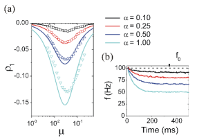
Figure 5: (Color online) Loss of linearity. (a) First SCC, $\rho_{1}$, as a function of the driving parameter $\mu$ in a perfect IF neuron model, for different adaptation strengths, $\alpha$. In all cases, $D=0.02~{}\text{ms}^{-1}$, $V_{\text{thr}}-V_{\text{r}}=1.0$, and $\tau_{\text{a}}=100.0~{}\text{ms}$. (b) As the value of $\alpha$ increases, the stationary firing rate decreases [asymptotic value of $f(t)$ at the right margin] and correspondingly, the adaptation effect is more prominent. In all cases, the driving drift is $\mu=0.10~{}\text{ms}^{-1}$ (which corresponds to a firing rate of $100~{}$ Hz in the absence of adaptation, $\alpha=0$), applied as a step function at time $t=0$ [see Fig. 1(b)]. Remaining parameters as in (a).

In the previous section we have shown that the onset of correlations has a specific structure and scales linearly with the adaptation strength, Eqs. (III.1) and (26). This scaling enables us to consider normalized SCC, $\hat{\rho}_{\text{k}}$, as shown in the preceding figures. However, for a large enough value of $\alpha$, higher-order effects become important and these equations are no longer applicable. In particular, given that the expression for $\rho_{1}$, Eq. (III.1), does not saturate we expect that higher-order effects oppose the linear growth. In Fig. 5(a) we show the (not normalized) first SCC, $\rho_{1}$, for different adaptation strengths. As expected, for small values of $\alpha$ the theoretical expression, Eq. (III.1), properly accounts for the linear scaling. Specifically, correlations grow linearly up to approximately $\alpha\approx 0.25$ [red symbols and line in Fig. 5(a)], which represents a frequency adaptation of about $20\%$ [see red line in Fig. 5(b)]. This limit is slightly better than that expected from the upper limit of the linear scaling in the stationary mean adaptation strength, $\langle\varepsilon\rangle$ [see Fig. 2(b)]. For larger values, higher effects are non-negligible and affect the correlations in the predicted manner. For a realistic SFA (adaptation of about $50\%$), the analytical expressions provide a qualitative agreement regarding the dependence on the parameters [shape of the curve in Fig. 5(a) as a function of $\mu$ or $D$], but only a rough estimate of the correct values of the correlations (cyan symbols and line in Fig. 5).

III.3 Spike-count variance reduction

The presence of negative correlations affects the spike-count variance. To analyze this effect, it is convenient to introduce the Fano factor, $\text{FF}_{T}$, which relates the mean and the variance of the spike counts observed in a temporal window of length $T$, $\langle n_{T}\rangle$ and $\langle\Delta n_{T}^{2}\rangle$, respectively, as the ratio

$$\text{FF}_{T}=\frac{\langle\Delta n_{T}^{2}\rangle}{\langle n_{T}\rangle}.$$ (27)

For point processes, the asymptotic behavior of the Fano factor reads cox

$$\text{FF}_{\infty}=\text{lim}_{T\rightarrow\infty}~{}\text{FF}_{T}=\text{CV}^{2}~{}\left(1+2\sum_{\text{k}=1}^{\infty}\rho_{\text{k}}\right),$$ (28)

where CV is the coefficient of variation, defined as the ratio between the standard deviation and the mean of the unconditional ISI statistics,

$$\text{CV}=\frac{\sqrt{\langle\Delta\tau^{2}\rangle}}{\langle\tau\rangle}.$$ (29)

Combining the preceding equations and given that $\langle n_{T}\rangle=T/\langle\tau\rangle$, the spike-count variance reads, in the asymptotic limit,

$$\langle\Delta n_{T}^{2}\rangle=\frac{\langle\Delta\tau^{2}\rangle}{\langle\tau\rangle^{3}}~{}\left(1+2\sum_{\text{k}=1}^{\infty}\rho_{\text{k}}\right)~{}T.$$ (30)

The linear growth in $T$ of the spike-count variance is a characteristic of a diffusive process (and the reason for the usefulness of the Fano factor). Inasmuch as the asymptotic limit is reached, it is useful to analyze the preceding factor, which we denote $\langle\hat{\Delta n_{T}^{2}}\rangle$,

$$\langle\hat{\Delta n_{T}^{2}}\rangle=\frac{\langle\Delta\tau^{2}\rangle}{\langle\tau\rangle^{3}}~{}\left(1+2\sum_{\text{k}=1}^{\infty}\rho_{\text{k}}\right).$$ (31)

Equation (31) highlights two contributions to the spike-count variance: a contribution from the FPT statistics related to a single spiking process, $\langle\Delta\tau^{2}\rangle/\langle\tau\rangle^{3}$, and a contribution from the ISI correlations provided by the entire spike train, $\left(1+2\sum_{\text{k}=1}^{\infty}\rho_{\text{k}}\right)$.

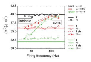
Figure 6: (Color online) Spike-count variability in the perfect IF neuron model, as a function of the firing frequency. The neuron without adaptation ($\alpha=0$) shows a spike-count variance that does not depend on the firing frequency [theoretical ($T$) and numerical ($N$) results are represented by a black thick line and open squares, respectively]. For $\alpha\neq 0$ ($\alpha=0.05$ and $\alpha=0.10$ in red and green, respectively) there is a reduction in the variance, which also is independent of the firing rate [theoretical ($T$) and numerical ($N$) results are shown by thick lines and empty symbols, respectively]. By shuffling the original spike train, from which the spike counts are drawn, we destroy the correlations. For the shuffled spike train, theoretical ($T$ sh.) and numerical ($N$ sh.) results are represented by hidden lines and semifilled symbols, respectively. Parameters: $V_{\text{thr}}-V_{\text{r}}=1.0$, $\tau_{\text{a}}=100.0~{}\text{ms}$, $D=0.02~{}\text{ms}^{-1}$. The driving parameter $\mu$ was varied from $0.005$ to $0.2~{}\text{ms}^{-1}$. Numerical results are presented as a function of the firing frequency observed from the mean spike counts. Theoretical results are shown as a function of the firing frequency computed from $f^{-1}=\langle\tau\rangle_{\phi_{0}}+\langle\varepsilon\rangle\langle\tau\rangle_{\phi_{1}}$. Numerical procedure: to compute the spike-count statistics, the length of the temporal window $T$ was varied for different values of $\mu$, checking in all cases that the asymptotic regime was reached. Numerical results were obtained from a single spike train with a temporal length $T_{\text{total}}=T~{}N_{\text{sample}}$, with $N_{\text{sample}}=100$. The value of $N_{\text{sample}}$ is low, due to the computational cost of the shuffling procedure. To improve the accuracy, results are presented as averages over $N_{\text{repet}}=500$ repetitions.

The effect of the adaptation strength $\alpha$ on the spike-count variance is twofold; it changes the ISI statistics as well as the correlations between the ISIs. In the slight adaptation regime we consider, the contribution to the spike-count variance due to the correlations is a linear term in $\alpha$. Explicitly, it is easy to show that

$$1+2\sum_{\text{k}=1}^{\infty}\rho_{\text{k}}=1+2\frac{\rho_{1}(\alpha)}{1-\phi_{0}^{L}(1/\tau_{\text{a}})},$$ (32)

where $\rho_{1}(\alpha)$ is given by Eq. (III.1). To be consistent with this description, the term provided by the ISI statistics should be linearized, and reads

$$\frac{\langle\Delta\tau^{2}\rangle}{\langle\tau\rangle^{3}}=\frac{\langle\Delta\tau^{2}\rangle_{\phi_{0}}}{\langle\tau\rangle_{\phi_{0}}^{3}}\hskip 145.10922pt$$

$$+\langle\varepsilon\rangle~{}\frac{\langle\tau^{2}\rangle_{\phi_{1}}-2\langle\tau\rangle_{\phi_{0}}\langle\tau\rangle_{\phi_{1}}-3\langle\Delta\tau^{2}\rangle_{\phi_{0}}\langle\tau\rangle_{\phi_{1}}/\langle\tau\rangle_{\phi_{0}}}{\langle\tau\rangle_{\phi_{0}}^{3}},$$ (33)

where $\langle\varepsilon\rangle$ is given by Eq. (11). Replacing the complete expressions for both factors [Eqs. (32) and (III.3)] in Eq. (31), and keeping the first order in $\alpha$ [$\langle\hat{\Delta n_{T}^{2}}\rangle\approx\mathcal{O}(\alpha)$], we obtain

$$\langle\hat{\Delta n_{T}^{2}}\rangle=\frac{\langle\Delta\tau^{2}\rangle_{\phi_{0}}}{\langle\tau\rangle_{\phi_{0}}^{3}}+\frac{\alpha}{[1-\phi_{0}^{L}(1/\tau_{\text{a}})]\langle\tau\rangle_{\phi_{0}}^{3}}\hskip 42.67912pt$$

$$\times\Bigg{[}\langle\tau^{2}\rangle_{\phi_{1}}-3\frac{\langle\tau^{2}\rangle_{\phi_{0}}\langle\tau\rangle_{\phi_{1}}}{\langle\tau\rangle_{\phi_{0}}}+\frac{\langle\tau\rangle_{\phi_{1}}}{1-\phi_{0}^{L}(1/\tau_{\text{a}})}\hskip 28.45274pt$$

$$\times\left(\langle\tau\rangle_{\phi_{0}}-3\langle\tau\rangle_{\phi_{0}}\phi_{0}^{L}(1/\tau_{\text{a}})-2\frac{d\phi_{0}^{L}(s)}{ds}\rfloor_{1/\tau_{\text{a}}}\right)\Bigg{]}.$$ (34)

It is clear that the independent term on the right-hand side of Eq. (III.3) corresponds to the asymptotic spike-count variance (normalized by $T$) of the neuron without adaptation ($\alpha=0$). Even when general in the regime we consider, the behavior of this rather complicated expression for $\alpha\neq 0$ is not obvious at all. The expression simplifies enormously for the case of the perfect IF neuron model. For this neuron, we have

$$\langle\hat{\Delta n_{T}^{2}}\rangle=\frac{2D}{(V_{\text{thr}}-V_{\text{r}})^{2}}-\frac{4D}{(V_{\text{thr}}-V_{\text{r}})^{3}}~{}\alpha.$$ (35)

Surprisingly, this expression for the spike-count variance reduction does not depend on the driving parameter $\mu$, which sets the firing frequency. In Fig. 6 we show this behavior for different values of the adaptation strength. The case $\alpha=0$ corresponds to a perfect IF neuron model without adaptation (black line and squares). As $\alpha$ increases, the spike-count variance decreases, and this effect does not depend on the firing frequency set by varying $\mu$. For $\alpha=0.05$, theoretical and numerical results agree (red thick lines and empty circles, respectively); whereas for $\alpha=0.10$ the flat reduction is numerically observed, but the appropriate variance decrease is just approximated by the theoretical prediction (green thick lines and empty triangles). The same holds true for higher adaptation strengths (not shown). As expected, since the expression for $\rho_{1}$ [Eq. (III.1)] and the exponential structure for higher lags [Eq. (26)] are approximate, the infinite sum in Eq. (32) amplifies a tiny error. In consequence, even when we have observed that $\rho_{1}$ is properly described by Eq. (III.1) for the case $\alpha=0.10$ [Fig. 5(a)], the expression for the spike-count variance [Eq. (35)] is qualitatively good but approximate [note, however, that there is a significant reduction even for small values of $\alpha$, and Eq. (35) has a moderate relative error for $\alpha=0.1$]. The linear spike-count variance reduction expressed by Eq. (35) is unbounded, which is obviously unreasonable (it enables negative values for the spike-count variance). Higher-order terms should oppose this linear reduction, as can be observed in Fig. 6 for the case $\alpha=0.10$.
Since the spike-count variance reduction for a given firing frequency arises from the interplay between the FPT statistics and the presence of correlations, it would be interesting to disentangle to what extent each effect contributes to the observed reduction. To analyze this question we shuffled the spike train, which maintains the first-order statistics (FPT statistics) destroying ISI correlations. The spike-count variance reduction for the shuffled spike train is shown in Fig. 6 as semifilled symbols. The theoretical analog corresponds to $\langle\hat{\Delta n_{T}^{2}}\rangle$ given exclusively by Eq. (III.3), since the sum of the SCC values is $0$ [$1+2\sum_{\text{k}=1}^{\infty}\rho_{\text{k}}=1$ instead of Eq. (32)], and it is shown as dashed lines in Fig. 6. As expected, theoretical and numerical results are in good accordance. The behavior observed for each contribution is reasonable. At low firing frequencies, within each ISI the exponential evolution of the adaptation process has decayed, meaning that each $\varepsilon_{\text{n}}=\alpha$ and correlations disappear. Correspondingly, the spike-count variance reduction is given exclusively by the FPT statistics (this case corresponds to $\tau_{\text{d}}\rightarrow 0$ in urdapilleta ; lindner2004b ), and we denote this regime as an intrinsic reduction in Fig. 6. At large firing frequencies, the adaptation process within a single ISI is essentially constant (i.e., $\tau_{\text{a}}\rightarrow\infty$). In this case, the collection of ISIs satisfies a quasistatic approximation urdapilleta2009 , and the spike-count variance of the shuffled spike train is indistinguishable from the case of no adaptation. However, in this limit, correlations decay very slowly [$\phi_{0}^{L}(1/\tau_{\text{a}})\rightarrow 1$; see Fig. 3(c)], and even when each SCC is small because $\rho_{1}$ is, the sum of correlations accumulates over many lags, building up a finite nonvanishing value. In Fig. 6, we denote this range as a reduction due to correlations (“corrs” in the figure).
Equation (35) shows that the spike-count variance reduction is independent of the firing frequency, for the perfect IF neuron model. As shown in the previous paragraph, in the limit of low as well as large firing frequencies, the mechanisms that account for the reduction are different. The fact that both effects influence the spike-count variance to the same extent, and furthermore, that these mechanisms exactly compensate each other at intermediate firing frequencies is intriguing. Obviously, these results hold for this particular IF model. It would be interesting to analyze the contributions in other IF models; we expect analogous spike-count variance reductions and the same limit behaviors, but not an independence on firing frequencies (in general, in other models the spike-count variance for $\alpha=0$ depends on the firing frequency).

IV Discussion and concluding remarks

In this work we have analyzed the onset of correlations for a general neuron model, where an external input as well as an internal spike-based adaptation current drive the membrane potential. The external current is composed by a static input and fast fluctuations. For this system, the dependence of the adaptation current on the past history, through the initial states of the adaptation process, facilitates the development of correlations between successive ISIs prescott2008 ; benda2010 ; wang1998 ; liu2001 ; avila2011 . In the regime of slight adaptation, we have shown that correlations share a general structure across different models. By means of a hidden Markov model, we have explicitly derived the dependence of the SCC on different properties of the FPT statistics corresponding to the underlying time-inhomogeneous stochastic process, Eqs. (III.1) and (26). In this regime, for one-dimensional models such as IF neuron models, the necessary properties are given urdapilleta ; comment1 ; lindner2004b ; lindner2005b . For any other (high-dimensional) model, whenever a slight exponential time-dependent current smoothly reshapes the FPT statistics in comparison to the unperturbed case (analogously to Fig. 1 in urdapilleta ), the expressions derived here apply. The geometric structure and exponential decay for the SCC is surprisingly simple and general for the scenario considered here. This kind of structure was first observed by Lindner and Schwalger for successive escapes of an overdamped Brownian particle in a randomly modulated asymmetric double well, which can be modeled as transitions between discrete states lindner2007 ; schwalger2008b . Posteriorly, these authors extended their results to a situation with multiple internal states schwalger2010b and, in particular, studied the case of negative correlations in neurons with inhibitory feedback (resembling current-based adaptation), with an appropriate scheme of transitions. Even when general and very promising, a quantitative evaluation of correlations in adapting neurons under this framework requires a procedure for the estimation of transition rates, in a discrete version of adaptation, obtained from dynamical models and/or experimental data. The results obtained here are in qualitative agreement to those obtained by Schwalger and Lindner schwalger2010b , which implies that this estimation procedure could be an interesting topic to study.
The development of negative correlations in successive ISIs in a spike train influences the encoding capabilities of a neural system avila2011 ; nawrot2007 ; nawrot2010 ; farkhooi2009 ; farkhooi2011 . Here, we have analyzed the decrease in the asymptotic spike-count variance due to the intrinsic variability reduction of the FPT statistics and the presence of correlations [Eqs. (31)-(III.3)] in comparison to the case without adaptation. In particular, for the perfect IF neuron model the decrease is extremely simple and does not depend on the firing frequency, Eq. (35). This analysis is theoretically important, but it should be put in the proper context. The spike-count variance reduction given by Eq. (31) is valid for the asymptotic limit, which can be unfeasible in real neurons, especially at low firing rates. For systems operating with finite temporal windows, the framework presented here should be extended by using the complete formalism derived by van Vreeswijk in vreeswijk , and finely used by Farkhooi et al. to analyze a population scheme farkhooi2011 . In this case, the spike-count variance will be a function of the length of the temporal window used to compute the statistics, and obviously, the results presented here should agree in the limit of large windows. This behavior was outlined by Chacron et al. in a different version of adaptation (see results of the model without slow noise in Fig. 4 of chacron2001 ). That work also highlighted a possible explanation to the interesting finding made by Ratnam and Nelson ratnam2000 , where the spike-count variance exhibits a minimum as a function of the length of the counting window (a possible behaviorally important phenomenon). In their work, Chacron et al. demonstrated that a slow external noise leaves relatively intact the short-range correlations, while destroying negative correlations at large lags, giving rise to small and slowly decaying positive correlations which dominate the asymptotic regime. On the other hand, across different neural systems it has been observed that the only significant SCC corresponds to the lag 1 avila2011 ; farkhooi2009 , which reinforces the idea that a slow external noise would be an important part of the incoming signal, in addition to fast fluctuations. Theoretically, the analysis of the spike-count variance for IF neuron models driven by slow fluctuations were successfully carried out via a quasistatic approximation middleton2003 ; schwalger2008a . This suggests that the hidden Markov model used here to model negative correlations could be extended with a similar quasistatic approximation in order to include slow fluctuations in the analysis.

V ACKNOWLEDGMENTS

The author thanks Inés Samengo for a critical reading of the manuscript. This work was supported by the Consejo de Investigaciones Científicas y Técnicas de la República Argentina.

References

- (1) E. R. Kandel, J. H. Schwartz, and T. M. Jessell, Principles of Neural Science (McGraw-Hill, New York, 2000).
- (2) B. Wark, B. N. Lundstrom, and A. Fairhall, Curr. Opin. Neurobiol. 17, 423 (2007).
- (3) B. Ermentrout, Neural Comput. 10, 1721 (1998).
- (4) J. Benda and A. V. M. Herz, Neural Comput. 15, 2523 (2003).
- (5) M. H. Higgs, S. J. Slee, and W. J. Spain, J. Neurosci. 26(34), 8787 (2006).
- (6) S. A. Prescott and T. J. Sejnowski, J. Neurosci. 28(50), 13649 (2008).
- (7) S. Chung, X. Li, and S. B. Nelson, Neuron 34, 437 (2002).
- (8) D. V. Madison and R. A. Nicoll, J. Physiol. 354, 319-331 (1984).
- (9) F. Helmchen, K. Imoto, and B. Sakmann, Biophys. J. 70, 1069-1081 (1996).
- (10) P. Sah, Trends Neurosci. 19(4), 150-154 (1996).
- (11) B. Hille, Ion Channels of Excitable Membranes, 2nd ed. (Sinauer Associates, Sunderland, MA, 1992).
- (12) J. Benda, A. Longtin, and L. Maler, J. Neurosci. 25(9), 2312 (2005).
- (13) J. Benda, L. Maler, and A.Longtin, J. Neurophysiol. 104, 2806 (2010).
- (14) X. -J. Wang, J. Neurophysiol. 79, 1549 (1998).
- (15) Y. -H. Liu and X. -J. Wang, J. Comput. Neurosci. 10, 25 (2001).
- (16) S. Peron and F. Gabbiani, Nature Neurosci. 12, 318 (2009).
- (17) S. P. Peron and F. Gabbiani, Biol. Cybern. 100, 505 (2009).
- (18) P. Dayan and L. F. Abbott, Theoretical Neuroscience: Computational and Mathematical Modeling of Neural Systems, (The MIT Press, Cambridge, MA, 2001).
- (19) O. Avila-Akerberg and M. J. Chacron, Exp. Brain Res. 210, 353 (2011).
- (20) D. R. Cox and P. A. W. Lewis, The statistical analysis of series of events (Methuen, London, 1966).
- (21) M. P. Nawrot, C. Boucsein, V. Rodriguez-Molina, A. Aertsen, S. Grün, and S. Rotter, Neurocomputing 70, 1717 (2007).
- (22) M. P. Nawrot, in Analysis of Parallel Spike Trains, edited by S. Grün and S. Rotter (Springer Series in Computational Neuroscience, Springer-Verlag, Berlin, 2010).
- (23) F. Farkhooi, M. F. Strube-Bloss, and M. P. Nawrot, Phys. Rev. E 79, 021905 (2009).
- (24) F. Farkhooi, E. Muller, and M. P. Nawrot, Phys. Rev. E 83, 050905 (2011).
- (25) M. J. Chacron, B. Lindner, and A. Longtin, Phys. Rev. Lett. 92(8), 080601 (2004).
- (26) B. Lindner, M. J. Chacron, and A. Longtin, Phys. Rev. E 72, 021911 (2005).
- (27) O. Ávila Åkerberg and M. J. Chacron, Phys. Rev. E 79, 011914 (2009).
- (28) W. H. Nesse, L. Maler, and A. Longtin, Proc. Natl. Acad. Sci. USA 107(51), 21973 (2010).
- (29) S. B. Lowen and M. C. Teich, Fractal-Based Point Processes (John Wiley & Sons, New Jersey, 2005).
- (30) S. B. Lowen and M. C. Teich, J. Acoust. Soc. Am. 92(2), Pt. 1, 803 (1992).
- (31) A. Longtin and D. M. Racicot, Biosystems 40, 111 (1997).
- (32) R. Ratnam and M. E. Nelson, J. Neurosci. 20(17), 6672 (2000).
- (33) M. J. Chacron, A. Longtin, and L. Maler, J. Neurosci. 21(14), 5328 (2001).
- (34) J. W. Middleton, M. J. Chacron, B. Lindner, and A. Longtin, Phys. Rev. E 68, 021920 (2003).
- (35) B. Lindner, Phys. Rev. E 69, 022901 (2004).
- (36) T. Schwalger and L. Schimansky-Geier, Phys. Rev. E 77, 031914 (2008).
- (37) T. Schwalger, K. Fisch, J. Benda, and B. Lindner, PLoS Comput. Biol. 6(12), e1001026 (2010).
- (38) E. Muller, L. Buesing, J. Schemmel, and K. Meier, Neural Comput. 19(11), 2958 (2007).
- (39) T. Schwalger and B. Lindner, Eur. Phys. J. Spec. Topics 187, 211 (2010).
- (40) B. Lindner and T. Schwalger, Phys. Rev. Lett. 98, 210603 (2007).
- (41) T. Schwalger and B. Lindner, Phys. Rev. E 78, 021121 (2008).
- (42) C. van Vreeswijk, in Analysis of Parallel Spike Trains, edited by S. Grün and S. Rotter (Springer Series in Computational Neuroscience, Springer-Verlag, Berlin, 2010).
- (43) E. Urdapilleta, Phys. Rev. E 83, 021102 (2011).
- (44) In urdapilleta we have found the FPT density function for the perfect IF model (Wiener process) with the exponential time-inhomogeneous drift supporting the subthreshold dynamics of the adaptation current. As pointed out in the conclusions of urdapilleta , the system of recurrence equations can be extended to other diffusion processes [here characterized by ]. In this case, the homogeneous part of the equations to solve, Eqs. (8) and (9) in urdapilleta , changes respectively. Given that the homogeneous part is the same for all order terms, the formal solution of each term is obtained from the Green’s function associated to the unperturbed system and the corresponding source.
- (45) B. Lindner, J. Stat. Phys. 117(3/4), 703 (2004).
- (46) B. Lindner and A. Longtin, J. Theor. Biol. 232, 505 (2005).
- (47) E. Urdapilleta and I. Samengo, Phys. Rev. E 80, 011915 (2009).