Distance Preserving Graph Simplification

Abstract

Large graphs are difficult to represent, visualize, and understand. In this paper, we introduce “gate graph” - a new approach to perform graph simplification. A gate graph provides a simplified topological view of the original graph. Specifically, we construct a gate graph from a large graph so that for any “non-local” vertex pair (distance higher than some threshold) in the original graph, their shortest-path distance can be recovered by consecutive “local” walks through the gate vertices in the gate graph. We perform a theoretical investigation on the gate-vertex set discovery problem. We characterize its computational complexity and reveal the upper bound of minimum gate-vertex set using VC-dimension theory. We propose an efficient mining algorithm to discover a gate-vertex set with guaranteed logarithmic bound. We further present a fast technique for pruning redundant edges in a gate graph. The detailed experimental results using both real and synthetic graphs demonstrate the effectiveness and efficiency of our approach.

I Introduction

Reducing graph complexity or graph simplification is becoming an increasingly important research topic [1, 32, 37, 34, 30]. It can be very challenging to grasp a graph even with thousands of vertices. Graph simplification targets at reducing edges, vertices, or extracting a high level abstraction of the original graph so that the overall complexity of the graph is lowered while certain essential properties of the graph can still be maintained. It has been shown that such simplification can help understand the underlying structure of the graph [13, 1]; better visualize graph topology [26, 13]; and speed up graph computations [2, 23, 7, 19, 33, 30].

In this paper, we investigate how to extract a set of vertices from a graph such that the vertex locations and relationships not only help to preserve the distance measure of the original graph, but also provide a simplified topological view of the entire graph. Intuitively, these vertices can be considered to distribute rather “evenly” in the graphs in order to reflect its overall topological structure. For any “non-local” vertex pair (distance higher than some threshold), their shortest-path distance can be recovered by consecutive “local” walks through these vertices. Basically, these vertices can be viewed as the key intermediate highlights of the long-range (shortest-path distance) connections in the entire graph. In other words, for any vertex to travel to another vertex beyond its local range, it can always use a sequence of these discovered vertices (each one being in the local range of its predecessor) to recover its shortest path distance to the destination. Thus, conceptually, this set of vertices form a “wrap” surrounding any vertex in the original graph, so that any long range (shortest-path) traffic goes through the “wrap”. From this perspective, these vertices are referred to as the gate vertices and our problem is referred to as the gate-vertex set discovery problem. Furthermore, these gate vertices can be connected together using only “local” links to form a gate graph. A gate graph not only reveals the underlying highway structure, but also can serve as a simplified view of the entire graph. Gate-vertex set and gate graph have many applications in graph visualization  [14, 5] and shortest path distance computation [33].

I-A Problem Definition

Let $G=(V,E)$ be an unweighted and undirected graph, where $V=\{1,2,...,N\}$ is the vertex set and $E\subseteq V\times V$ is the edge set of graph $G$. We use $(u,v)$ to denote the edge from vertex $u$ to vertex $v$, and $P_{v_{0},v_{p}}=(v_{0},v_{1},...,v_{p})$ to denote a simple path from vertex $v_{0}$ to vertex $v_{p}$. The length of a simple path in unweighted graph is the number of edges in the path. For weighted graph, each edge $e\in E$ is assigned a weight $w(e)$. The length of a simple path in a weighted graph is the sum of weights from each edge in the path. The distance from vertex $u$ to vertex $v$ in the graph $G$ is denoted as $d(u,v)$, which is the minimal length of all paths from $u$ to $v$.

Given a user-defined threshold $\epsilon>0$, for any pair of connected vertices $u$ and $v$, if their distance is strictly less than $\epsilon$ ($d(u,v)<\epsilon$), we refer to them as a local pair, and their distance is referred to as a local distance; if their distance is higher than or equal to $\epsilon$ but finite, we refer to them as a non-local pair, and their distance is referred to as a non-local distance. In addition, we also refer to $\epsilon$ as the locality parameter or the granularity parameter.

Definition 1

(Minimum Gate-Vertex Set Discovery (MGS) Problem) Given an unweighted and undirected graph $G=(V,E)$ and user-defined threshold $\epsilon>0$, vertex set $V^{\ast}\subseteq V$ is called a gate-vertex set if $V^{\ast}$ satisfies the following property: for any non-local pair $u$ and $v$ ($d(u,v)\geq\epsilon$), there is a vertex sequence formed by consecutive local pairs from $u$ to $v$, $(u,v_{1},v_{2},\cdots,v_{k},v)$ where $v_{1},v_{2},\cdots,v_{k}\in V^{\ast}$, such that $d(u,v_{1})<\epsilon$, $d(v_{1},v_{2})<\epsilon$, $\cdots$ , $d(v_{k},v)<\epsilon$, and $d(u,v_{1})+d(v_{1},v_{2})+\cdots+d(v_{k},v)=d(u,v)$. The gate vertex set discovery problem seeks a set of gate vertices with smallest cardinality.

In other words, the gate-vertex set guarantees that the distance between any non-local pair $u$ and $v$ can be recovered using the distances from source vertex $u$ to a gate vertex $v_{1}$, between consecutive gate vertices, and from the last gate vertex $v_{k}$ to the destination vertex $v$. These are all local distances. Here, the local distance requirement for recovering any non-local distance enables the gate vertices to reflect enough details of the underlying topology of the original graph $G$. Based on the gate-vertex set, we can further define the gate graph.

Definition 2

(Minimum Gate Graph Discovery (MGG) Problem) Given an unweighted and undirected graph $G=(V,E)$ and a gate-vertex set $V^{\ast}$ ($V^{\ast}\subseteq V$) with respect to parameter $\epsilon$, the gate graph $G^{\ast}=(V^{\ast},E^{\ast},W)$ is any weighted and undirected graph where $W$ assign each edge $e\in E^{\ast}$ a weight $w(e)$, such that for any non-local pair $u$ and $v$ in $G$ ($d(u,v)\geq\epsilon$), we have $d(u,v)=$

$$min_{d(u,x)<\epsilon\wedge d(y,v)<\epsilon\wedge x,y\in V^{\ast}}d(u,x)+d(x,y|G^{\ast})+d(y,v);$$

Here $d(x,y|G^{\ast})$ is the distance between $x$ and $y$ in the weighted gate graph. The gate graph discovery problem seeks the gate graph with the minimum number of edges. Note that the edges in the gate graph may not belong to the original graph.

Our Contributions:

1) We introduce and formally define the new gate-vertex set and gate graph discovery problems, which are applicable to numerous graph mining tasks;

2) Based on basic properties of gate vertices, we perform a theoretical study on gate-vertex set by connecting it to the theory of VC-dimension, and prove NP-hardness of minimum gate-vertex set discovery problem;

3) We develop an efficient mining algorithm based on the set-cover framework to discover the gate-vertex set with guaranteed logarithmic approximation bound. We discuss a fast approach to prune redundant edges in gate graph;

4) We perform a detailed experimental evaluation using both real and synthetic graphs. Our results demonstrate the effectiveness and efficiency of our approach.

II Related Problems and Work

Graph Simplification: Our work on discovering a gate-vertex set and gate graph can be categorized as graph simplification with focus on preserving shortest path distance measure. The most intuitive graph simplification method is graph clustering [1] or decomposition [25], which provides a high-level view of the graphs. However, this approach mainly focuses on discovering the community structure of the graph, and its representation is generally too coarse to preserve many other essential information of the graphs (such as the connectivity and shortest-path distance measure). Several recent efforts study how to simplify the graphs while maintaining its key graph properties, such as the effective resistance [32], connectivity [37], and other path-oriented measures [34]. However, in these studies, the simplified graph is a spanning subgraph of the original graph, and thus does not reduce the overall scale of the graph in terms of the number of vertices. In our work, we instead focus on discovering a subset of essential vertices which can maximally recover the all-pair shortest-path distances with respect to the locality parameter $\epsilon$.

In order to better visualize a large graph, the visualization community has proposed several methods to simplify graphs. For instance, authors in  [26] consider sampling a subgraph from the original graph for visualization, and in [13], the authors develop a pruning framework to remove unimportant vertices in terms of their betweenness and other distance-related measures. These methods are in general heuristically-oriented and cannot provide quantitative guarantee on how good the graph properties are preserved. Our gate-vertex set and gate graph provide a new means to visualize large graphs and assist distance-centered graph visualization and analysis.

Finally, several works [6, 35, 15, 20] study how to extract a concise subgraph which can best describe the relationship between a pair or a set of vertices in terms of electric conductance [6, 35] or network reliability [15, 20]. Our goal is to depict the shortest-path distances using gate vertices and gate graph.

Shortest-Path Distance Computation: Computing shortest-path distance is a fundamental task in graph mining and management. Many important graph properties, such as graph diameter, betweenness centrality and closeness centrality, are all highly dependent on distance computation. Even though the BFS approach for computing pair-wise distance is quite efficient for small graphs, it is very expensive for large graphs. Leveraging the highway structure to speed up the distance computation has been shown to be quite successful in road-network and planar graphs [17, 18, 29, 33]. The recent $k$-skip graph [33] work represents the latest effort in using highway structure to reduce the search space of the well-known shortest distance computation method, Reach [11]. Basically, each shortest path is succinctly represented by a subset of vertices, namely $k$-skip shortest path, such that it should contain at least one vertex out of every $k$ consecutive vertices in the original shortest path. In other words, $k$-skip shortest path compactly describes original shortest path by sampling its vertices with a rate of at least $1/k$. Tao et al. show that those sampled vertices can be utilized to speed up the distance computation. Following the similar spirit, gate-vertex set and gate graph directly highlight the long-range connection between vertices, and can also serve as a highway structure in the general graph.

We note that the $k$-skip cover and gate vertices are conceptually close but different. The $k$-skip cover intends to uniformly sample vertices in shortest paths, whereas the gate-vertex set tries to recover shortest-path distance using intermediary vertices (and local walks). More importantly, the $k$-skip cover focuses on the road network and implicitly assume there is only one shortest path between any pair of vertices [33]. In this work, we study the generalized graph topology, where there may exist more than one shortest path between two vertices which is very common in graphs such as a social network. Our goal is to recover the non-local distance between any pair of vertices using only one shortest path. Finally, in this paper, we focus on developing methods to discover minimum gate-vertex set, whereas [33] only targets at a random set of vertices which forms a $k$-skip cover, i.e., the minimum $k$-skip cover problem is not addressed.

Landmarks: Landmark vertices (or simply landmarks) are a subset of vertices in the graph which are selected and utilized for graph navigation (particularly shortest-path distance computation) [8, 24, 21, 10, 27, 22, 4] and transformation (multidimensional scaling) [5]. Given a landmark set, each vertex in the graph can approximate its network “position” by its distances to each landmark. Thus, each vertex is directly mapped to a multidimensional space where each landmark corresponds to a unique dimension. In online shortest-path distance computation, landmarks have been used together with triangle inequality for pruning search space [10]; several studies directly utilize landmarks for distance estimation [21, 27, 22, 4]. However, the landmarks generally are not necessarily good representatives for highlighting the underlying topology of the entire graphs, while the gate vertices explicitly ensure any pair-wise distance can be recovered through user-defined granularity threshold.

Vertex Separators: Vertex separators [28] are a set of vertices (denoted as $S$) in a graph $G$ which partition the entire vertex set $V$ into three sets, $A$, $S$ and $B$, where there are no edges between vertices in $A$ and $B$. Using vertex separators, a graph can be decomposed recursively. This is often used as a basis for applying a divide-and-conquer approach to (hard) graph problems. The gate vertices are different from separators as they do not have to explicitly partition the graphs. In particular, if there are multiple non-local shortest paths between two vertices, the gate vertices will guarantee to recover at least one of them. Thus, the gate vertices in some sense relax the condition of vertex separators and thus allow us to recover the shortest-path distance even on general graphs.

III Properties of Gate-Vertex Set and Problem Transformation

Based on the definition of the gate-vertex set, to verify that a given set of vertices $V^{\ast}$ is a gate-vertex set, the naïve approach is to explicitly verify that the distance between every non-local pair $(u,v)$ can be recovered through some sequence of consecutive local pairs: ($u,v_{1}$), ($v_{1},v_{2}$), $\cdots$, ($v_{k},v$), where all intermediate vertices $v_{1},v_{2},\cdots,v_{k}\in V^{\ast}$. Clearly, this can be expensive and difficult to directly apply to discover the minimum number of gate vertices. In Subsection III-A, we first discuss an alternative (and much simplified) condition, which enables the discovery of gate-vertex set using only local distance, and reveal the NP-hardness of minimum gate-vertex set discovery problem. In addition, we utilize the VC-dimension theory to bound the size of gate vertices.

III-A Local Condition and Problem Reformulation

In order to design a more efficient and feasible algorithm, we explore the properties of gate vertices and observe that gate-vertex set can be efficiently checked by a very simple condition. Let $G=(V,E)$ be an unweighted and undirected graph. For any vertex $u\in V$, its $\epsilon$-neighbors, denoted as $N_{\epsilon}(u)$ is a set of vertices such that their distances to $u$ is no greater than $\epsilon$, i.e., $N_{\epsilon}(u)=\{v\in V|0<d(u,v)\leq\epsilon\}$. Let $L$ be a set of vertices and $S=\{(u_{0},v_{0}),...,(u_{k},v_{k})\}$ be a set of vertex pairs in the graph $G$. We say that $L$ covers $S$ if for each vertex pair $(u_{i},v_{i}){\color[rgb]{0,0,0}\in S}$ there is at least one vertex $x\in L$ such that $d(u_{i},v_{i})=d(u_{i},x)+d(x,v_{i})$.

Now, we introduce the following key observation:

Lemma 1

(Sufficient Local Condition for MGS) If for each vertex $x$ in the graph $G$, there is a subset of vertices $L(x)\subseteq N_{\epsilon-1}(x)$ which covers all vertex pairs $\{(x,y_{i})|d(x,y_{i})=\epsilon\}$, then $\bigcup_{x\in V}L(x)$ is a gate-vertex set of graph $G$. In other words, a vertex set which covers any pair of vertices with distance $\epsilon$ is a gate-vertex set.

Proof Sketch:For any non-local pair $s$ and $t$ ($d(s,t)\geq\epsilon$), we denote one of their shortest paths to be $P=(s=v_{0},v_{1},\cdots,v_{k}=t)$ with the length $k=d(s,t)\geq\epsilon$. Let us consider $v_{\epsilon}$ on the shortest path. Since $d(s,v_{\epsilon})=\epsilon$, there is at least one vertex $x_{0}\in L(s)$, such that $d(s,x_{0})+d(x_{0},v_{\epsilon})=d(s,v_{\epsilon})$. Now, we consider two cases:

1) If $d(x_{0},t)<\epsilon$, then we recover a local-walk sequence ($s,x_{0},t$).

2) If $d(x_{0},t)\geq\epsilon$, since $d(s,x_{0})+d(x_{0},t)=d(s,t)$ (based on the fact $d(x_{0},v_{\epsilon})+d(v_{\epsilon},t)=d(x_{0},t)$), we have $d(x_{0},t)<d(s,t)$. Then, we can recursively apply the above method to identify $x_{1}$ between $x_{0}$ and $t$, $x_{2}$ between $x_{1}$ and $t$, until $d(x_{i},t)<\epsilon$.

Since $x_{0},x_{1},\cdots,x_{i}\in\bigcup_{x\in V}L(x)$ (i.e. they also belong to $V^{\ast}$) and the distance of every vertex pair $(x_{m},x_{m+1})$ is less than $\epsilon$, we can recover the distance between $s$ and $t$ to be $(s,x_{0},x_{1},\cdots,x_{i},t)$, where $d(s,x_{0})<\epsilon$, $d(x_{0},x_{1})<\epsilon$, $\cdots$, $d(x_{i},t)<\epsilon$ and $d(s,x_{0})+\sum_{m=0}^{i-1}d(x_{m},x_{m+1})+d(x_{i},t)=d(s,t)$. Therefore, $\bigcup_{x\in V}L(x)$ or any set of vertices $V^{\prime}$ which can cover any vertex pair with distance $\epsilon$, is a gate-vertex set. $\Box$

Interestingly, this local condition specified in Lemma 1 is also a necessary one for a gate-vertex set.

Lemma 2

(Necessary Local Condition for MGS) Given an unweighted and undirected graph $G$ and its gate-vertex set $V^{\ast}$ with respect to parameter $\epsilon$, for any vertex $s\in V$, we have $L(s)=\{x\in V^{\ast}|0<d(s,x)<\epsilon\}$ such that for any vertex $t$ with distance $\epsilon$ to $s$ (i.e., $d(s,t)=\epsilon$), there is $x\in L(s)$ with $d(s,t)=d(s,x)+d(x,t)$.

Proof Sketch:For any non-local vertex pair $(s,t)$ with $d(s,t)=\epsilon$, by the definition of gate-vertex set, there must exist a sequence of vertices $x_{0},x_{1},...,x_{i}\in V^{\ast}$, such that $d(s,t)=d(s,x_{0})+d(x_{0},x_{1})+...+d(x_{i},t)$ where $d(s,x_{0})<\epsilon$, $\cdots$, $d(x_{i},t)<\epsilon$. Since $d(s,x_{0})<\epsilon$, we have $x_{0}\in L(s)$. Also, it is easy to see that $d(s,t)=d(s,x_{0})+d(x_{0},t)$ because $d(s,t)-d(s,x_{0})=d(x_{0},x_{1})+...+d(x_{i},t)\geq d(x_{0},t)$ and $d(s,t)\leq d(s,x_{0})+d(x_{0},t)$. Therefore, we have at least $x_{0}\in L(s)$ satisfying $d(s,t)=d(s,x_{0})+d(x_{0},t)$. $\Box$

Putting this together, given parameter $\epsilon$, checking whether a subset of vertices $V^{\ast}\subseteq V$ is gate-vertex set is equivalent to checking the following condition: for any vertex pair $(u,v)$ with distance $\epsilon$, there is a vertex $x\in V^{\ast}$ such that $d(u,v)=d(u,x)+d(x,v)$. Similarly, we can rewrite the minimum gate-vertex set discovery problem in the following equivalent local condition (only covering vertex pairs with distance $\epsilon$).

Definition 3

(Minimum Gate-Vertex Set Problem using Local Condition) Given unweighted undirected graph $G=(V,E)$ and user-defined threshold $\epsilon$, we would like to seek a set of vertices $V^{\ast}$ with minimum cardinality, such that any pair of vertices $(u,v)$ with distance $\epsilon$ is covered by at least one vertex $x\in V^{\ast}$: $d(u,x)+d(x,v)=d(u,v)$.

In the following, we would like to prove NP-hardness of aforementioned problem by reducing the 3SAT problem.

Theorem 1

(NP-hardness of MGS using Local Condition provided Shortest Paths) Given a collection $P$ of vertex-pair $(u,v)$ with $d(u,v)=\epsilon$ denoting a set of shortest paths from unweighed undirected graph $G=(V,E)$, finding minimum number of vertices $V^{\ast}\subseteq V$ such that any vertex-pair $(u,v)$ is covered by at least one vertex $x\in V^{\ast}$ is NP-hard.

Proof Sketch:We can reduce 3SAT problem to this problem. Let $S$ be an instance of 3SAT with $n$ variables $x_{1}$, $x_{2}$, …, $x_{n}$, and $m$ clauses $C_{1}$, $C_{2}$, …, $C_{m}$. We show that an instance of our problem can be constructed correspondingly as follows. A unweighted undirected graph $G$ consisting of a vertex $p$ and a set of variable gadgets and clause gadgets will be generated.

The variable gadget with respect to variable $x$ contains $3$ vertices and $2$ edges:

1) $3$ vertices: $b^{x}$, $b^{\overline{x}}$ and $e^{x}$;

2) $2$ edges: $(b^{x},e^{x})$ and $(b^{\overline{x}},e^{x})$.

Also, we add edges $(p,b^{x})$ and $(p,b^{\overline{x}})$ to build the connections between $p$ and variable $x$’s gadget. For each clause $C_{i}=(X,Y,Z)$, we add vertex $c_{i}$ to graph $G$ first. Then, if $X=x$, we add edge $(b^{x},c_{i})$, otherwise, we add edge $(b^{\overline{x}},c_{i})$. The same rule is applied to literals $Y$ and $Z$. Next we add 3 edges $(b^{X},c_{i})$, $(b^{Y},c_{i})$ and $(b^{Z},c_{i})$ into $G$. The subgraph containing vertices $\{p,b^{X},b^{Y},b^{Z},c_{i}\}$ and above created edges is called clause gadget regarding $C_{i}$.

Here we consider $\epsilon=2$ in the graph $G$. That is, we try to find a set of vertices $V^{\ast}$ with minimum cardinality to cover a collection $P$ of shortest path with length $\epsilon$ (i.e., 2 in this scenario). Note that, in our problem, for shortest path $SP=(x,y,z)$ with length $2$, only vertex $y$ in the middle can be used to cover $SP$ identified by its two endpoints $(x,z)$. Let us define $P_{pe_{i}^{x}}$ to be vertex pairs indicating shortest paths with length $2$ between $p$ and $e^{x}$. Moreover, $P_{pc_{k}}$ denotes vertex pairs representing shortest paths with length $2$ between $p$ and $c_{k}$. We consider gate-vertex selection problem on vertex pairs $P=(\cup_{i}P_{pe^{x_{i}}})\bigcup(\cup_{k}P_{pc_{k}})$ .

In the following, we prove that above 3SAT instance is satisfiable if and only if the instance of our problem has a solution of size at most $n$. We need to prove both the “only if” and the “if” as follows.

$\Longrightarrow$: Suppose 3SAT instance $S$ is satisfiable and $f$ is its corresponding satisfying assignment. For each variable $x$, if $f(x)=1$, vertex $b^{x}$ is added to $S^{\ast}$ to cover the shortest paths within $P_{pc_{i}}$ where clause $C_{i}$ contains $x$ or $\overline{x}$. Otherwise, we add vertex $b^{\overline{x}}$ into $S^{\ast}$. As we can see, either $b^{x}$ or $b^{\overline{x}}$ is selected, shortest paths within $P_{pe_{i}^{x}}$ always can be covered. On the other hand, since one of literals $X$ in each clause $C$ is guaranteed to be true, there is always one vertex indicating such literal serves as intermediate hop in shortest paths of $P_{pc}$. In this sense, only one vertex corresponding to the literal with true value is added to $V^{\ast}$ in each variable gadget. Therefore, the solution size for the instance of our problem is $n$.

$\Longleftarrow$: Suppose graph $G$ has a gate-vertex set $V^{\ast}$ of size $n$ with respect to $\epsilon=1$. For 3SAT instance $S$, we define a truth assignment by setting $f(x)=1$ if and only if vertex $b^{x}$ is included in $V^{\ast}$. We will show this is satisfying assignment without conflict. First, according to the definition of gate-vertex set, there are at least one vertex from $V^{\ast}$ cover vertex pair $P_{pc_{i}}$, meaning that there are at least one literal with truth value existing in each clause. This leads to the truth value of entire 3SAT instance. Furthermore, in order to cover every vertex pair $P_{pe^{x_{i}}}$, either vertex $b^{x_{i}}$ or $b^{\overline{x_{i}}}$ must be chosen. Considering the constraint $|V^{\ast}|\leq n$, for each variable gadget, only one of $b^{x_{i}}$ and $b^{\overline{x_{i}}}$ can be included in gate-vertex set. From the perspective of 3SAT instance $S$, this guarantees that only one of literals $x_{i}$ and $\overline{x_{i}}$ would be assigned with true value. That is, no conflict occurs in our aforementioned assignment. Putting both together, we can claim that $f$ is a satisfying truth assignment. $\Box$

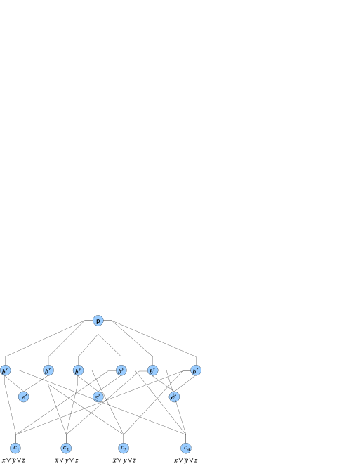
Figure 1: Example for proof of Theorem 1

Example: consider the following boolean formula $S$ in 3SAT problem with respect to variables $x$ $y$ and $z$:

$$(x\vee\overline{y}\vee\overline{z})\wedge(\overline{x}\vee y\vee z)\wedge(\overline{x}\vee y\vee\overline{z})\wedge(x\vee\overline{y}\vee z)$$

To simplify the discussion, we name the above 4 clauses as $C_{1}$ $C_{2}$ $C_{3}$ and $C_{3}$, respectively. Here, we consider the vertex pairs $P=\{(p,e^{x}),(p,e^{y}),(p,e^{z}),(p,c_{1}),(p,c_{2}),(p,c_{3}),(p,c_{4})\}$ with distance $\epsilon$ (i.e., 2 in the example). The constructed graph $G$ including variable gadgets and clause gadgets is shown in Figure 1. In this example, the formula is satisfied by the assignment $x=1$, $y=1$ and $z=0$. According to the rule defined in the proof, we add $b^{x}$, $b^{y}$ and $b^{\overline{z}}$ to gate-vertex set $V^{\ast}$. It is not hard to verify that no vertex set with less vertices compared to $|V^{\ast}|$ can be obtained. From another direction, we can see that $V^{\ast}=\{b^{\overline{x}},b^{\overline{y}},b^{z}\}\subseteq V(G)$ is minimum gate-vertex set with respect to vertex pairs in $P$ (i.e., the problem is equivalent to find the set cover problem: ground set $\{c_{1},c_{2},c_{3},c_{4}\}$, candidate sets $\{b^{X},b^{Y},b^{Z}\}$ ($X\in\{x,\overline{x}\}$, $Y\in\{y,\overline{y}\}$ and $Z\in\{z,\overline{z}\}$)). The corresponding satisfying assignment can be build as follows: $x=0$, $y=0$ and $z=1$. It is straightforward to verify that this is a truth assignment for instance $S$.

III-B Size of Minimum Gate-Vertex Set

In the following, using the theory of VC-dimension, we derive an upper bound of the cardinality of minimum gate-vertex set.

VC-dimension and $\epsilon$-net: We start with a brief introduction of the VC-dimension of set systems and $\epsilon$-net. The notion of VC-dimension originally introduced by Vladimir Vapnik and Alexey Chervonenkis in [36] is widely used to measure the expressive power of a set system. Let $U$ be a finite set and $R$ a collection of subsets of $U$, the pair $(U,R)$ is referred to be a set system. A set $A\subseteq U$ is shatterable in $R$ if and only if for any subset $S$ of $A$, there is always a subset $X\in R$ where $X\cap A=S$. In other words, $X$ contains the “exact” $S$ with no element in $A\backslash S$. Then, we say the VC-dimension of set system $(U,R)$ is the largest integer $d$ such that no subset of $U$ with size $d+1$ can be shattered. In addition, given parameter $\epsilon\in[0,1]$, a set $N\subseteq U$ is an $\epsilon$-net on $(U,R)$ if for any subset $X\in R$, $X$ has size no less than $\epsilon|U|$, the set $N$ contains at least one element of $X$. For the set system with bounded VC-dimension $d$, the $\epsilon$-net theorem states there exists a $\epsilon$-net with size $O(\frac{d}{\epsilon}\log\frac{1}{\epsilon})$ [12].

Using the VC-dimension and $\epsilon$-net theorem, we can bound the size of minimum gate-vertex set.

Theorem 2

Given graph $G=(V,E)$ with parameter $\epsilon$, the size of minimum gate-vertex set is bounded by $O(\frac{|V|}{\epsilon-1}\log\frac{|V|}{\epsilon-1})$.

To prove Theorem 2, we need a few lemmas. To facilitate our discussion, we introduce the following notations. Given the input graph $G=(V,E)$, let $p^{\ast}_{s,t}$ be the subpath of shortest path $p_{s,t}$ without the two endpoints. For instance, if $p_{s,t}=(s,u,...,v,t)$, its corresponding $p^{\ast}_{s,t}=(u,...,v)$. Further, let $P_{l}$ only contains shortest path $p_{s,t}$ of length $l$, i.e., $P_{l}=\cup_{s,t}\{p_{s,t}\text{ s.t. }|p_{s,t}|=l\}$. Given $P_{l}$ with $l\geq 1$, we say $P^{\ast}_{l}$ is a core-set of $P_{l}$ if for each shortest path $p_{s,t}$, only its subpath $p^{\ast}_{s,t}$ is included in $P^{\ast}_{l}$, i.e., $P^{\ast}_{l}=\cup_{s,t}\{p^{\ast}_{s,t}\text{ s.t. }p_{s,t}\in P_{l}\}$.

We first establish the relationship between $\epsilon$-net and gate-vertex set.

Lemma 3

($\frac{\epsilon-1}{|V|}$-net) Given a set system $(V,P^{\ast}_{\epsilon})$, where $P_{\epsilon}$ contains a shortest path for every vertex pair with distance $\epsilon$ in graph $G=(V,E)$ ($P^{\ast}_{\epsilon}$ is the core-set of $P_{\epsilon}$), a $\frac{\epsilon-1}{|V|}$-net $V^{\ast}$ of $(V,P^{\ast}_{\epsilon})$ is a gate-vertex set.

Proof Sketch:By definition of $P^{\ast}_{\epsilon}$, the number of vertices in shortest path $p_{u,v}\in P^{\ast}_{\epsilon}$ is $\epsilon-1$. According to definition of $\frac{\epsilon-1}{|V|}$-net, for each shortest path $p_{s,t}\in P^{\ast}_{\epsilon}$, we have $p_{s,t}\cap V^{\ast}\neq\emptyset$. Moreover, recall that each shortest path of $P^{\ast}_{\epsilon}$ is a subpath of some shortest paths of $P_{\epsilon}$ by removing two endpoints. In other words, if $V^{\ast}$ contains at least one vertex from each shortest path in $P^{\ast}_{\epsilon}$, then at least one vertex from shortest path in $P_{\epsilon}$ is included in $V^{\ast}$. Since $P_{\epsilon}$ contains one shortest path for every vertex pair with distance $\epsilon$, this satisfies the condition of gate-vertex set such that there is at least one vertex $x\in V^{\ast}$ holding $d(u,v)=d(u,x)+d(x,v)$ for every vertex pair $(u,v)$ with $d(u,v)=\epsilon$. Therefore, $V^{\ast}$ is a gate-vertex set. $\Box$

To bound the size of $\epsilon$-net, the VC-dimension of the set system is needed. In  [9, 33], the VC-dimension of a unique shortest path system, i.e., only one shortest path exists between any pair of vertices in a graph, is studied. Formally, we first define Unique Shortest Path System:

Definition 4

(Unique Shortest Path System (USPS)) [9] Given a graph $G=(V,E)$ and a collection $Q$ of shortest paths from $G$, we say $Q$ is a unique shortest path system if: any vertex pair $u$ and $v$ is contained in two shortest paths $p_{s_{1},t_{1}},p_{s_{2},t_{2}}\in Q$, then they are linked by the same path, i.e., $p_{u,v}=p^{\prime}_{u,v}$, where $p_{u,v}$ ($p^{\prime}_{u,v}$) is the subpath of $p_{s_{1},t_{1}}$ ($p_{s_{2},t_{2}}$).

For any unique shortest path system $(V,P)$, it can be easily verified that its VC-dimension is $2$ [9, 33]. Thus, if a graph contains only one unique shortest path system, then, the bound described in Theorem 2 can be directly derived (following the $\epsilon$-net theorem [12]). However, in our problem, there can be many different shortest paths between any given pair of vertices. To deal with this problem, we make the following observation:

Lemma 4

(Existence of USPS) Given any graph $G=(V,E)$, there exists a unique shortest path system $P$ in $G$.

Proof Sketch:We prove this lemma by induction on the edge size of graph $G$. We first assume that when a graph $G$ has $|E|=N$ edges, it has a unique path system $P$. Now, we add a new edge $e=(x,y)$ in $E$ (the new edge can introduce a new vertex, the new graph is denoted as $G^{\prime}$), Then, we first drop all the $p_{u,v}\in P$ ($P$ is in $G$), such that $p_{u,v}$ is not the shortest path between $u$ an $v$ any more, i.e., $|p_{u,v}|>d(u,v|G^{\prime})$. Clearly, the remaining $P$ is still a unique shortest path system. Now, for the dropped vertex pair $u$ and $v$, we must be able to construct a new shortest path between $u$ and $v$ using edge $e=(x,y)$ as follows: $p_{u,x}\cup(e=(x,y))\cup p_{y,v}$, where $p_{u,x}$ and $p_{y,v}$ belong to the remaining $P$. By adding those new shortest paths to $P$, we claim $P$ is the unique shortest path system containing a shortest path between any vertex pairs in $G^{\prime}$. This is because for any vertex pair $s$ and $t$, either they has a shortest path which does not contain new edge $e$ or contains. For both cases, their shortest path is uniquely defined in the new path system. $\Box$

Basically, we can always extract a USPS from a general graph even when there are more than one shortest path between any pair of vertices. Combining Lemma 3 and  4, we now can prove Theorem 2.

Proof Sketch of Theorem 2: By lemma 4, for any graph $G=(V,E)$, we have unique shortest path systems $P_{\epsilon}$ and $P^{\ast}_{\epsilon}$, because they are subsets of general USPS $P$ with all possible length. Now, for the set system $(V,P^{\ast}_{\epsilon})$, we know that: 1) its VC-dimension is at most 2 [9, 33]; 2) $\frac{\epsilon-1}{|V|}$-net on this set system is a gate-vertex set by lemma 3. Using $\epsilon$-net theorem, we have a gate-vertex set (i.e., $\frac{\epsilon-1}{|V|}$-net) of size $O(\frac{|V|}{\epsilon-1}\log\frac{|V|}{\epsilon-1})$. Moreover, the size of minimum gate-vertex set is no larger than any gate-vertex set. Putting both together, the theorem follows. $\Box$

Figure 2: Gate-vertex set ($\epsilon=3$)

Lower Bound: The lower bound of the minimum gate-vertex set can be arbitrarily small. For example, in Figure 2, minimum gate-vertex set is only central vertex, and no gate vertex is needed for any graph with diameter less than $\epsilon$. In this case, even a gate-vertex set of size $O(\frac{|V|}{\epsilon-1}\log\frac{|V|}{\epsilon-1})$ is obtained, we still cannot decide how good it is compared to the minimum gate-vertex set.

IV Algorithms for Gate-Vertex Set Discovery

Based on Theorem 2 and $\epsilon$-net theorem  [12], we observe that any random sample with size $O(\frac{|V|}{\epsilon-1}\log\frac{|V|}{\epsilon-1})$ has high probability to form a gate-vertex set but does not have a guarantee. An adaptive sampling method  [33] is introduced to guarantee to find a $k$-skip cover. The guarantee is achieved by choosing a vertex using the information gained from previously sampled vertices. Since a $k$-skip cover can serve as a candidate for the gate-vertex set with $\epsilon=k+1$ (as stated in Lemma 5), we can utilize the adaptive sampling method to discover gate-vertex set. However, since the lower bound of the minimum gate-vertex set can be arbitrarily small, the approximation ratio between the size of the gate-vertex set discovered by this method and the minimum one is not bounded. In other words, this method does not necessarily produce tight gate-vertex set.

Lemma 5

Given graph $G=(V,E)$, if parameters $\epsilon$ of gate-vertex set and $k$ of $k$-skip cover satisfy condition $k=\epsilon-1$, $k$-skip cover $V^{\ast}$ is a gate-vertex set.

Proof Sketch:We prove it by way of contradiction. Let us assume $V^{\ast}$ is not gate-vertex set, meaning, there exists a vertex pair $(u,v)$ with distance $d(u,v)=\epsilon$ and we do not have one vertex $x\in V^{\ast}$ (note that $x\neq u,v$) such that $d(u,v)=d(u,x)+d(x,v)$. By definition of $k$-skip cover, we guarantee to have one shortest path $p_{u,v}$ in which $V^{\ast}$ contains at least one vertex out of every consecutive $k$ vertices. Therefore, for $p_{u,v}$, only starting point $u$ and ending point $v$ are allowed to be included in $V^{\ast}$. However, even both $u$ and $v$ are selected, $V^{\ast}$ still does not contain any vertex from subpath $p_{u^{\prime},v^{\prime}}$ with $k$ vertices (since $p_{u,v}$ has $k+2$ vertices). This reaches a contradiction. $\Box$

Note that a gate-vertex set with locality parameter $\epsilon=k+1$ may not be a $k$-skip cover. Also, as we mentioned earlier, the $k$-skip cover focuses on the unique shortest path system, and since there may exist more than one shortest path between two vertices, the adaptive sampling method chooses one of such paths arbitrarily.

We propose a set-cover-based algorithm with guaranteed logarithmic bound and compare it with the adaptive sampling method.

IV-A Set-Cover Based Approach

We propose an effective algorithm based on set cover framework to discover gate-vertex set with logarithmic bound. Specially, we transform the minimum gate-vertex set discovery problem (MGS) to an instance of set cover [3] problem: Let $U=\{(u,v)|d(u,v)=\epsilon\}$ be the ground set, which includes all the non-local pairs with distance equal to $\epsilon$. Each vertex $x$ in the graph is associated with a set of vertex pairs $C_{x}=\{(u,v)|d(u,v)=d(u,x)+d(x,y)=\epsilon\}$, where $C_{x}$ includes all of the non-local pairs with distance equal to $\epsilon$ and there is a shortest path between them going through vertex $x$. Given this, in order to discover the minimum gate-vertex set, we seek a subset of vertices $V^{\ast}\in V$ to cover the ground set, i.e., $U=\bigcup_{v\in V^{\ast}}{\color[rgb]{0,0,0}C_{v}}$, with the minimum cost $|V^{\ast}|$. Basically, $V^{\ast}$ serves as the index for the selected candidate sets to cover the ground set.

Theorem 3

The minimum solution $V^{\ast}$ for the above set-cover instance is a minimum gate-vertex set of graph $G$ with parameter $\epsilon$.

Its proof can be easily followed by Definition 3. The minimum set cover problem is NP-hard, and we can apply the classical greedy algorithm [3] for this problem: Let $R$ records the covered pairs in $U$ (initially, $R=\emptyset$). For each possible candidate set $C_{x}=\{(u,v)|d(u,v)=d(u,x)+d(x,y)=\epsilon\}$ discussed above, we define the price of $C_{x}$ as:

$$\gamma(C_{x})=\frac{1}{|C_{x}\setminus R|}$$

At each iteration, the greedy algorithm picks the candidate set $C_{x}$ with the minimum $\gamma(C_{x})$ (the cheapest price) and put its corresponding vertex $x$ in $V^{\ast}$. Then, the algorithm will update $R$ accordingly, $R=R\cup C_{x}$. The process continues until $R$ completely covers the ground set $U$ ($R=U$), which contains all non-local pairs with distance equal to $\epsilon$. It has been proved that the approximation ratio of this algorithm is $ln(|U|)+1$ [3].

Fast Transformation: In order to adopt the aforementioned set-cover based algorithm to discover the gate-vertex set, we first have to generate the ground set $U$ and each candidate subset $C_{x}$ associating with vertex $x$. Though we only need the non-local pairs with distance $\epsilon$, whose number is much smaller than all non-local pairs, the straightforward approach still needs to precompute the distances of each pair of vertices with distance no greater than $\epsilon$, and then apply such information to generate each candidate set. For large unweighted graphs, such computational and memory cost can still be rather high.

Here, we introduce an efficient procedure which performs a local BFS for each vertex to visit only its $\epsilon$-neighborhood and during this process to collect all information needed for constructing the set-cover instance ($U$ and $C_{x}$, for $x\in V$). Specifically, for each local BFS starting from a vertex $u$, it has the following two tasks: 1) it needs to find all the vertices which is exactly $\epsilon$ distance away from $u$, and then add them into $U$; and 2) for each such pair $(u,v)$ ($d(u,v)=\epsilon$), it needs to identify all the vertices $x$ which can appear in a shortest path from $u$ to $v$. In order to achieve these two tasks, we again utilize the basic recursive property of the shortest-path distance: Let vertex $y$ to $u$’s distance be $d$ and $z\neq u$ be vertex whose distance to $u$ is $d-1$, we know all the intermediate vertices appearing in at least one shortest path from $u$ to $z$ (denoted as $I(z)$). Then, all the intermediate vertices on shortest paths from $u$ to $y$ can be written as $\bigcup_{(z,y)\in E}(I(z)\cup\{z\})$. Based on this property, we can easily maintain $I(x)$ for each vertex $x$ such that $1<d(u,x)<\epsilon$; when $d(u,x)=1$, $I(x)=\emptyset$. Since BFS visits $u$’s $\epsilon$-neighborhood in a level-wise fashion, when it reaches the $\epsilon$ level, where each vertex $v$ is $\epsilon$ distance to $u$, we not only get each targeted pair $(u,v)$, but also get $I(v)$, which we can easily use for producing the candidate set: for each $x\in I(v)$, we add $(u,v)$ to $C_{x}$.

Algorithm 1 sketches the BFS-based algorithm for constructing the set cover instance. Especially, set $I(v)$ is computed in Line $5$, and when BFS reaches the $\epsilon$ level (Line $11$), it adds $(u,v)$ to the ground set $U$ (Line $12$) and to each $C_{x}$ ($x\in I(v)$) (Line $13$). The algorithm will be invoked for each vertex $u$ in the graph. Finally, Figure 3 illustrates a simple running example of Algorithm 1 for vertex $u$ with $\epsilon=3$.

Algorithm 1 BFSSetCoverConstruction($G=(V,E)$,$\epsilon$,$U$,$u$)

1:  $I(u)\leftarrow\emptyset$; $level(u)\leftarrow 0$; $Q\leftarrow\{x\}$ {queue for BFS};

2:  while $Q\neq\emptyset$ do

3:     $u\leftarrow Q.pop()$;

4:     if $level(v)\geq 2$ {$d(u,v)\geq 2$} then

5:        $I(v)\leftarrow\bigcup_{(x,v)\in E\wedge level(x)+1=level(v)}I(x)\cup\{x\}$

6:     end if

7:     for all $v\in Neighbor(u)$ {$(u,x)\in E$} do

8:        if $v$ is not visited then

9:           if $level(v){\color[rgb]{0,0,0}<}\epsilon$ {$d(u,v){\color[rgb]{0,0,0}<}\epsilon$} then

10:              $Q.push\_back(v)$;

11:           else

12:              $U\leftarrow U\cup\{(u,v)\}$;

13:              $\forall x\in I(v)$, $C_{x}\leftarrow C_{x}\cup\{(u,v)\}$;

14:           end if

15:        end if

16:     end for

17:  end while

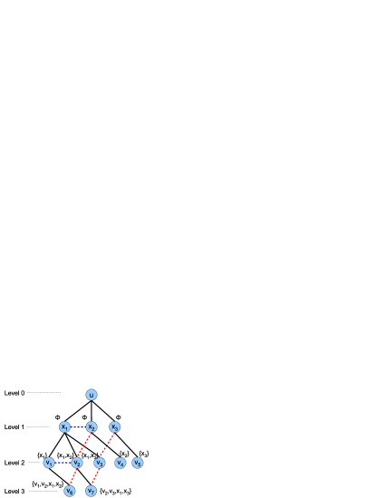
(a) Example for Algorithm 1

(b) Example for Set Cover

Figure 3: Example for Gate Discovery Algorithm ($\epsilon=3$)

Computational Complexity: The overall set-cover based mining algorithm for discovering gate-vertex set includes two key steps: 1) Constructing set-cover instance (Algorithm 1) and 2) the greedy set-cover discovering algorithm. The first step for collecting ground set and each candidate set takes $O(\sum_{v\in V}(|N_{\epsilon}(v)|^{2}+|E_{\epsilon}(v)|))$, where $|N_{\epsilon}(v)|$ ($|E_{\epsilon}(v)|$) is the number of vertices (edges) in the $v$’s $\epsilon$-neighborhood. For the greedy set cover procedure, by utilizing the speedup queue technique [31, 16], we only need to visit $d\ll|V|$ vertices in the queue (i.e., all vertices are ranked in ascending order in the queue), and each step takes $O(d(\log|V|+1))$ time to exact and update the queue. As greedy procedure has $O(|V^{\ast}|)$ steps, it takes $O(d|V^{\ast}|(\log|V|+1))$ in total. Putting together, the overall algorithm’s time complexity is $O(d|V^{\ast}|\log|V|+\sum_{v\in V}|N_{\epsilon}(v)|^{2})$.

V Algorithm for Gate Graph Discovery

In this section, we study the gate graph discovery problem (Definition 2 in Subsection I-A). Basically, after a gate-vertex set $V^{\ast}$ is discovered from graph $G$, we ask how to minimally connecting those gate vertices while still preserving the ability of representing non-local distances through consecutive local pairs? Specifically, the gate graph $G^{\ast}=(V^{\ast},E^{\ast},W)$ is a weighted graph, which guarantees for any non-local pair $u$ and $v$ in $G$ ($d(u,v)\geq\epsilon$), $d(u,v)=$

$$min_{d(u,x)<\epsilon\wedge d(y,v)<\epsilon\wedge x,y\in V^{\ast}}d(u,x)+d(x,y|G^{\ast})+d(y,v);$$

Here $d(x,y|G^{\ast})$ is the distance between $x$ and $y$ in the gate graph. To find the overall sparsest gate graph $G^{\ast}$ seems to be a hard problem. Here, we develop a two-stage algorithm to try to maximally prune non-essential edges between gate vertices.

Stage 1: Constructing Local-Gate Graph. In the first stage, for each gate vertex $u\in V^{\ast}$, we construct a local-gate graph $G^{\prime}$ by connecting two gate vertices only if their distance is less than $\epsilon$: $G^{\prime}=(V^{\ast},E^{\prime},W)$, where $E^{\prime}=\{(u,v)|d(u,v){\color[rgb]{0,0,0}<}\epsilon\}\subseteq V^{\ast}\times V^{\ast}$, and $w(u,v)=d(u,v)$ for $(u,v)\in E^{\prime}$. In the next stage, we will try to sparsify the local-gate graph by removing those non-essential edges, i.e., those edges whose removal will not affect any shortest-path distance in the gate graph. Why we need only local-pairs edges in the gate graph? Lemma 6 answers this question.

Lemma 6

The local-gate graph $G^{\prime}$ can guarantee that for any non-local pair $u$ and $v$ in $G$ ($d(u,v)\geq\epsilon$), $d(u,v)=$

$$min_{d(u,x)<\epsilon\wedge d(y,v)<\epsilon\wedge x,y\in V^{\ast}}d(u,x)+d(x,y|G^{\prime})+d(y,v);$$

Lemma 6 can be derived directly from the definition of gate-vertex set. Its proof is omitted for simplicity.

Stage 2: Edge Sparsification for Local-Gate Graph. In this stage, for each edge in the local-gate graph, we will determine whether removing it will change the distance between any local pair (if local pair is unchanged, so does non-local pair based on the definition of gate vertices). This can be equivalently described in the following condition: for any edge $(u,v)$ in the local-gate graph $G^{\prime}$, if there is a vertex $x$ ($x\neq u,x\neq v$), and $d(u,x)+d(x,v)=d(u,v)$, then, edge $(u,v)$ is non-essential and can be safely removed from $G^{\prime}$. How do we test this condition? Using the local-gate graph, this becomes very simple!

Lemma 7

Given local-gate graph $G^{\prime}$, let $N(u)$ be the adjacent gate vertices of vertex $u$ in $G^{\prime}$. For any edge $(u,v)$ in $G^{\prime}$, if there is a common vertex $x\in N(u)\cap N(v)$, such that $w(u,x)+w(x,v)=d(u,v)$, then, removing edge $(u,v)$ from $G^{\prime}$ will not affect the distance between any two vertices in $G^{\prime}$; if not, then, edge $(u,v)$ is essential and removing it increases the distance between at least one pair of vertices ($u$ and $v$).

This lemma essentially utilizes the property that in the local-gate graph, any pair with distance less than $\epsilon$ is linked through an edge in $G^{\prime}$ and thus we do not need to consider the situation where an edge can be replaced by a shortest path. Here, if an edge can be replaced, there must be a shortest path with only two edges. Given this, we can see that the pruning algorithm needs to scan the edge set of local-gate graph twice: 1) it applies Lemma 7 to determine whether an edge can be removed and flag them; and 2) it removes all the edges being flagged to be non-essential. Note that we should not drop an edge immediately after we found it to be non-essential since it can be used by testing other edges. Finally, the computational complexity of the overall edge sparsification algorithm is $O(\sum_{v\in V}(|N_{\epsilon-1}(v)|+|E_{\epsilon-1}(v)|)+|E^{\prime}|)$ considering the cost of computing the distance between local pairs of the gate vertices.

VI Experimental Evaluation

In this section, we empirically study the performance of our approaches on both real and synthetic datasets. Specifically, we compare two methods in the experiments: 1) FS, which corresponds to the approach utilizing adaptive sampling [33] for gate vertices discovery; 2) SC, which corresponds to the approach using set cover framework for gate vertices discovery (Subsection IV-A). Here, we are interested in understanding how many vertices can be reduced by the gate-vertex set and how many edges are needed in the gate graph, and how they are affected by the locality parameter $\epsilon$? In each experiment, we measure the number of gate vertices and the number of edges in gate graph, and the running time of algorithms. To gain a better understanding of experimental results, we also report two important graph measures: diameter (refer to as Diam.) and average value of pairwise shortest distances (refer to as Avg.Dist), for each graph. We implemented our algorithms in C++ and Standard Template Library (STL). All experiments were conducted on a 2.8GHz Intel Xeon CPU and 12.0GB RAM running Linux 2.6.

Dataset	#V	#E	Dia.	Avg.Dist
CA-GrQc	5242	28980	17	6.1
CA-HepTh	9877	51971	18	6
Wiki-Vote	7115	103689	7	3.3
P2PG08	6301	20777	9	4.6
P2PG09	8114	26013	9	4.8
P2PG30	36682	88328	11	5.7
P2PG31	62586	147892	11	5.9

TABLE I: Real Datasets

VI-A Real Data

In this subsection, we collect 7 real-world datasets listed in Table I to validate the performance of our approaches. Among them, CA-GrQc and CA-HepTh are collaboration networks from arXiv describing scientific collaboration relationships between authors in General Relativity and Quantum Cosmology field, and in High Energy Physics field, respectively. Moreover, P2PG08, P2PG09, P2PG30 and P2PG31 are $4$ snapshots of the Gnutella peer-to-peer file sharing network collected in August and September 2002, respectively. Wiki-Vote describes the relationships between users and their related discussion from the inception of Wikipedia until January 2008. All datasets are publicly available at Stanford Large Network Dataset Collection .

Table II reports the size of gate-vertex set and the number of edges in gate graphs by varying locality parameter $\epsilon$ from $3$ to $6$. Their corresponding shortest distance distribution and vertex degree distribution are shown in Figure VI-A and Figure VI-A, respectively. Since the distances and vertex degrees of P2PG30 and P2PG31 have similar distribution with that of P2PG08 and P2PG09, and their large values would affect other datasets’ distribution visualization, we omit them in both figures. We make the following observations:

Size of Gate-Vertex Set: Table II shows that the sizes of gate-vertex set discovered by both FS and SC are consistently smaller than that of original graphs. Among them, SC always obtains the better results, which are on average approximately $76\%$, $65\%$, $63\%$ and $56\%$ of the one from FS with $\epsilon$ ranging from $3$ to $6$. For SC approach, the size of gate-vertex set by SC is on average around $26\%$, $21\%$, $27\%$ and $24\%$ of the corresponding original graph when $\epsilon$ varies from $3$ to $6$. We also observe that, as locality parameter $\epsilon$ increases, the number of gate vertices discovered by SC is gradually reduced. Particularly, reduction ratios of CA-GrQc, CA-HepTh and Wiki-Vote are consistently better than that of P2P08, P2P09, P2P30 and P2P31. In Figure VI-A, CA-GrQc, CA-HepTh and Wiki-Vote seem to fit the power-law degree distribution very well, while there are a significant portion of vertices with degree ranging from $10$ to $15$ in P2P08, P2P09, P2P30 and P2P31. In other words, there exists a small portion of vertices with high degree potentially serving as the intermediate connectors for traffics between a large portion of vertex pairs in CA-GrQc, CA-HepTh and Wiki-Vote. By SC’s gate vertices discovery method using set cover framework, those vertices can be selected as gate vertices and thus dramatically simplify original graphs. However, for file-sharing network, a relatively large number of vertices with high connectivity potentially leads to larger size of gate-vertex set by the same selection principle. From the perspective of application domains, the results of SC on three social networks (i.e., CA-GrQc, CA-HepTh and Wiki-Vote) suggest a small highway structure capturing major non-local communications in the network. Interestingly, the consistent decreasing trends regarding the size of gate-vertex set with increasing $\epsilon$ are not observed in the results of FS on P2P30 and P2P31. Since adaptive sampling approach follows the spirit of greedy algorithm - choosing each gate vertex only based on local information, the mis-selection of gate vertices at earlier stages probably leads to significant increase of gate vertices at later stages. In other words, some important vertices selected as gate vertices in the procedure with small $\epsilon$ might be missed in the procedure with larger $\epsilon$. Therefore, it is reasonable to observe that the number of gate vertices discovered by FS unexpectedly becomes larger when $\epsilon$ increases.

Edge Size of Gate Graph: The number of edges in original graphs are significantly reduced by SC on three datasets CA-GrQc, CA-HepTh and Wiki-Vote. Especially, on average, the number of edges in gate graphs generated by SC are $6.5$, $6$, $6.3$ and $6$ times smaller than that of original graphs for $\epsilon$ to be $3$, $4$, $5$ and $6$. Besides that, SC still outperforms FS on those datasets, such that the number of edges in gate graphs by SC are on average about $49\%$, $51\%$, $53\%$ and $48\%$ of the one from gate graph by FS ranging $\epsilon$ from $3$ to $6$. Interestingly, as $\epsilon$ becomes larger, the number of edges in gate graphs generated by SC increases on CA-GrQc and CA-HepTh. The reason is, in order to guarantee that shortest paths between all non-local vertex pairs can be recovered utilizing fewer gate vertices, more edges are needed to build stronger connections among gate vertices. However, the number of edges in gate graphs generated by FS on CA-GrQc and CA-HepTh becomes smaller when $\epsilon$ increases. This demonstrates the effectiveness of edge sparsification algorithm for pruning redundant edges, since some of gate vertices discovered by FS are non-essential and are not necessarily to be connected to its $\epsilon$ neighbors. For other four datasets (P2P08, P2P09, P2P30 and P2P31), gate graphs generated by FS from those datasets contains fewer edges compared to the one of SC. Overall, they are on average about $1.3$, $1.1$, $1.4$ and $1.8$ times smaller than that of SC varying $\epsilon$ from $3$ to $6$. Also, as $\epsilon$ increases, the number of edges in gate graphs generated by both approaches on those four datasets increases. This is consistent with our earlier discussion that in these graphs, their interactions seem to be more random and the relatively large number of vertices with degrees between $10$ to $15$ may increase their chance to connect to other vertices with local walks.

Running Time: We take $\epsilon=3$ as an example. The running time of FS for all $7$ datasets are $65$ms, $132$ms, $3$s, $127$ms, $158$ms, $447$ms and $811$ms. The running time of SC are $23$s, $53$s, $1166$s, $183$s, $293$s, $279$s and $661$s for CA-GrQc, CA-HepTh, Wiki-Vote, P2P08, P2P09, P2P30 and P2P31, respectively. As locality parameter $\epsilon$ increases, the computational cost of both approaches become larger, because more vertex pairs should be considered in SC and more vertices would be traversed in FS. The average running time of SC on $\epsilon=5$ can cost up to a few hours, which is around $100$ times slower than that of FS. Indeed, the selection between FS and SC is a trade-off between reduction ratio and efficiency. In general, we can see that with rather smaller $\epsilon$ ($2$ or $3$), the vertex reduction by SC is quite significant which is also much better than that of FS, and their running time are reasonable in practice. In contrast to FS, the size of gate-vertex set discovered by SC is guaranteed to hold logarithmic approximation bound. Therefore, we would say SC with smaller $\epsilon$ is applicable in most of applications.

Dataset	$\epsilon=3$				$\epsilon=4$				$\epsilon=5$				$\epsilon=6$
	$\#V$		$\#E$		$\#V$		$\#E$		$\#V$		$\#E$		$\#V$		$\#E$
	FS	SC	FS	SC	FS	SC	FS	SC	FS	SC	FS	SC	FS	SC	FS	SC
CA-GrQc	2836	869	9266	2655	1625	655	6848	2933	1116	567	5580	2984	908	500	5192	2858
CA-HepTh	5131	2208	15831	7674	3381	1669	14921	10241	2525	1364	14316	11249	2134	1157	14476	11456
Wiki-Vote	2564	1598	84607	59132	2457	879	85051	34736	2236	584	83681	22652	2964	571	193913	19571
P2P08	2359	2340	10892	10738	2313	1920	23787	25406	2082	1584	26497	40218	2043	1095	28002	49139
P2P09	2930	2904	13633	13394	2874	2474	30219	32976	2643	2047	34870	53851	2556	1530	37022	75113
P2P30	9688	9627	37708	36708	10874	8820	98194	92820	8713	7551	108720	151677	8914	6845	127565	232971
P2P31	16493	16394	64624	146765	18248	14996	161883	155099	14745	12847	182599	256578	14895	11738	215742	383725

TABLE II: Sizes of Simplified Graph on Real Datasets

Dataset	$\epsilon=3$				$\epsilon=4$				$\epsilon=5$				$\epsilon=6$				$\epsilon=7$
	$\#V$		$\#E$		$\#V$		$\#E$		$\#V$		$\#E$		$\#V$		$\#E$		$\#V$		$\#E$
	FS	SC	FS	SC	FS	SC	FS	SC	FS	SC	FS	SC	FS	SC	FS	SC	FS	SC	FS	SC
sf2_10K	5781	5499	10559	7931	4648	4273	14067	15847	4057	3523	17175	21206	3754	3015	20258	26123	3495	2547	22127	32003
sf3_10K	6627	6203	18824	14926	5673	5208	29760	36385	5239	4437	39216	55411	4920	3457	46244	86414	4655	1264	50130	64944
sf4_10K	7190	6661	27721	22485	6406	5797	47198	61880	5992	4763	63681	103913	5737	1593	72145	124394	5211	800	92447	56418
sf5_10K	7647	7012	37339	30257	6968	6229	64952	89829	6641	4220	86701	204039	6315	802	96952	32989	5876	0	308613	0
sf6_10K	7912	7278	46570	38437	7315	6539	84063	120231	7035	2266	110166	218814	6686	789	123614	59338	5969	0	863493	0

TABLE III: Sizes of Simplified Graph on Scale-free Graphs

Dataset	$\epsilon=3$				$\epsilon=4$				$\epsilon=5$				$\epsilon=6$				$\epsilon=7$
	$\#V$		$\#E$		$\#V$		$\#E$		$\#V$		$\#E$		$\#V$		$\#E$		$\#V$		$\#E$
	FS	SC	FS	SC	FS	SC	FS	SC	FS	SC	FS	SC	FS	SC	FS	SC	FS	SC	FS	SC
rand2_10K	6243	5442	11523	7303	5158	4400	16627	18510	4709	3793	20557	27434	4386	3430	24200	36691	4165	3053	27296	47571
rand3_10K	7131	6340	20095	13863	6351	5449	33016	42290	5925	4873	43733	67867	5688	4071	52679	117127	5489	1933	57828	231900
rand4_10K	7727	6910	29142	21027	7108	6134	51635	72715	6801	5378	69228	130750	6608	2122	80754	305901	6348	830	90710	70541
rand5_10K	8157	7294	38769	28824	7629	6572	71324	106953	7367	4654	96131	287915	7170	847	108997	92646	6618	9	147143	36
rand6_10K	8452	7560	48476	36858	8005	6958	91149	142715	7797	2190	121549	278487	7607	802	134621	88650	6533	0	252001	0

TABLE IV: Sizes of Simplified Graph on Erdös-Rényi Random Graphs

Figure 4: Distance Distrib.(Real Graph)

Figure 5: Degree Distrib. (Real Graph)

Figure 6: Distance Distrib. (Scale-free Graph)

Figure 7: Distance Distrib. (Erdös-Rényi Graph)

Figure 8: Gate-Vertex Size (Large Rand Graph)

Figure 9: Edge Size in Gate Graph (Large Rand Graph)

VI-B Synthetic Data

In the following, we study two approaches on Scale-Free and Erdös-Rényi random graphs.

Scale-Free Random Graph: In this experiment, we generated a set of scale-free random graphs such that vertex degree follows power-law distribution using a publicly available graph generator . The number of vertices in those graphs are $10K$, and their edge density (i.e., $|E|/|V|$) ranges from $2$ to $6$. The diameter of those graphs are $10$, $8$, $7$, $6$, $6$, and their average pairwise distance are $6.4$, $5.1$, $4.5$, $4.2$ and $3.9$.

We can see from Table III, when locality parameter $\epsilon$ increases, the size of gate-vertex set discovered by both approaches consistently decreases for graphs with different edge density. Similar to the observation in the real-world datasets, SC always achieves better results than FS in terms of the number of gate vertices. Overall, the size of gate-vertex set discovered by SC is on average around $93\%$, $90\%$, $69\%$, $40\%$ and $28\%$ of the one of FS with $\epsilon$ from $3$ to $7$. In addition, as edge density increases, when locality parameter $\epsilon$ less than $Avg.Dist$, more gate vertices are discovered by both FS and SC in denser graphs. For denser graphs, since graph diameter becomes smaller, much more vertex pairs with distance $\epsilon$ need to be covered compared to sparse graphs (see Figure VI-A). Therefore, more gate vertices are required to serve as intermediate hops for any vertex pair. When $\epsilon$ is greater than $Avg.Dist$, the number of gate vertices discovered by SC is dramatically reduced since fewer vertex pairs need to be processed in set cover framework (e.g., sf5_10K and sf6_10K with $\epsilon\geq 6$). However, this phenomena is not observed in the results of FS, i.e., their gate-vertex sets are reduced very slowly. Even when $\epsilon$ is greater than diameter, no gate vertex is actually needed while FS still discovers lots of gate vertices (e.g., sf5_10K and sf6_10K with $\epsilon=7$). In terms of the number of edges in gate graphs, FS performs slightly better than SC. When locality parameter $\epsilon$ is less than $Avg.Dist$, the results on both FS and SC consistently increase following the opposite trend of the number of gate vertices. With the increase of $\epsilon$, fewer gate vertices are discovered and more internal connections within gate graph should be built to guarantee that there is a shortest path between any pair of gate vertices.

In terms of running time, when edge density increases, running times of both approaches are consistently increased. Taking $\epsilon=3$ as example, running time of SC for scale-free graphs with density from $2$ to $6$ are $6$s, $49$s, $158$s, $531$s and $1067$s, respectively. The running time of FS for those graphs are $85$ms, $170$ms, $232$ms, $344$ms and $471$ms, respectively. As $\epsilon$ becomes larger, longer running time is expected due to more vertices will be visited in both SC (i.e., procedure BFSSetCoverConstruction) and FS (i.e., breath-first-search). When $\epsilon=6$, the running time of SC is on average around $30$ times longer than that of $\epsilon=3$, ranging from $430$s to $6617$s. Also, running time of FS with $\epsilon=6$ is significantly increased which varies from $18$s to $1966$s. As $\epsilon$ increases, the efficiency advantage of FS over SC is dramatically reduced. This is caused by the explosive increase on the running time of FS’s edge sparsification, since the number of edges in local-gate graph of SC is much smaller than that of FS when $\epsilon\geq 6$.

Erdös-Rényi Random Graph: In this experiment, we generate a set of random graphs based on Erdös-Rényi model, with the edge density from $2$ to $6$, while keeping the number of vertices at $10K$. The diameter of those random graphs are $14$, $10$, $8$, $7$ and $6$, respectively. Also, their corresponding average pairwise distance are $6.8$, $5.3$, $4.7$, $4.3$ and $4.0$, respectively. Their shortest distance distribution is presented in Figure VI-A. By varying $\epsilon$ from $3$ to $7$, Table IV shows the number of vertices and the number of edges in simplified graphs with respect to original graphs with different edge density. The observations for both approaches SC and FS on scale-free graphs are still hold on Erdös-Rényi random graphs. Overall, the sizes of gate-vertex set discovered by SC are on average approximately $88\%$, $86\%$, $66\%$, $41\%$ and $30\%$ of the one from FS with $\epsilon$ from $3$ to $7$. In terms of the number edges in gate graphs, FS achieves slightly better results than SC. When $\epsilon$ is no less than $4$, the number of edges in gate graphs with different edge density by SC are on average $1.3$, $2$, $1.8$ and $1.6$ times greater than that of FS, respectively. Given the same $\epsilon$ and edge density, the size of gate-vertex set from scale-free graph discovered by both approaches are slightly smaller than that of Erdös-Rényi graphs. This is true for the number of edges in gate graphs as well, when $\epsilon$ is no less than $3$.

In general, the running time of both approaches on Erdös-Rényi graphs are faster than that of scale-free graphs. Especially, since for relatively large $\epsilon$, the size of gate-vertex set discovered by SC is significantly smaller than that of FS, we also observe that FS takes longer time than SC on those datasets with large value of $\epsilon$.

Large Random Graph: Finally, we perform this experiment on a set of Erdös-Rényi random graphs and scale-free random graphs with average edge density of 2, and we vary the number of vertices from $100K$ to $500K$. The locality parameter $\epsilon$ is specified to be $4$. The number of vertices and the number of edges in gate graphs are shown in Figure VI-A and Figure 9, respectively. The diameter of 5 Erdös-Rényi graphs are $18$, $18$, $19$, $19$, $21$, and their average values of pairwise distance are $8.4$, $8.9$, $9.2$, $9.4$ and $9.6$. For $5$ scale-free graphs, their diameter are $12$, $13$, $13$, $14$, $15$, and average values of pairwise distance are $7.8$, $8.2$, $8.4$, $8.6$ and $8.7$.

As we can see, the size of gate-vertex set discovered by SC is consistently smaller than that of FS in both types of graphs, while FS outperforms SC in terms of the number of edges in gate graphs. Moreover, as the number of vertices in original graphs increases, the size of gate-vertex set discovered by SC grows slower than that of FS. For both FS and SC, the number of discovered gate vertices from scale-free graphs are smaller than the one from Erdös-Rényi graphs.

Overall, we observe that the reduction ratio of gate vertices on the real-world graphs is significantly better than that of the synthetic graphs. This suggests that in the real world graphs, its underlying structure is not that “random”. In other words, the real graphs seems to have more recognizable “highway” structure in terms of the shortest path connection. From this perspective, the existing research on random graph generators have not been able to model this network behavior.

VII Conclusion

In this paper, we study a new graph simplification problem to provide a high-level topological view of the original graph while preserving distances. Specifically, we develop an efficient algorithm utilizing recursive nature of shortest paths and set cover framework to discover gate-vertex set. More interestingly, our theoretical results and algorithmic solution can be naturally applied for minimum $k$-skip cover problem, which is still open problem. In the future, we would like to study whether approximate distance with guaranteed accuracy can be gained based on our framework. We also want to investigate how our simplified graph can be applied for graph clustering, multidimensional scaling and graph visualization.

References

- [1] Charu C. Aggarwal and Haixun Wang. A survey of clustering algorithms for graph data. In Charu C. Aggarwal and Haixun Wang, editors, Managing and Mining Graph Data, volume 40, pages 275–301. Springer US, 2010.
- [2] Therese C. Biedl, Brona Brejová, and Tomás Vinar. Simplifying flow networks. In Proceedings of the 25th International Symposium on Mathematical Foundations of Computer Science, MFCS ’00, pages 192–201, 2000.
- [3] V. Chv tal. A greedy heuristic for the set-covering problem. Math. Oper. Res, 4:233–235, 1979.
- [4] Atish Das Sarma, Sreenivas Gollapudi, Marc Najork, and Rina Panigrahy. A sketch-based distance oracle for web-scale graphs. In WSDM ’10, pages 401–410, 2010.
- [5] Vin de Silva and Joshua B. Tenenbaum. Global Versus Local Methods in Nonlinear Dimensionality Reduction. In S. Becker, S. Thrun, and K. Obermayer, editors, Advances in Neural Information Processing Systems 15, pages 705–712, 2003.
- [6] Christos Faloutsos, Kevin S. McCurley, and Andrew Tomkins. Fast discovery of connection subgraphs. In KDD, pages 118–127, 2004.
- [7] Tomás Feder and Rajeev Motwani. Clique partitions, graph compression and speeding-up algorithms. In Proceedings of the twenty-third annual ACM symposium on Theory of Computing, STOC ’91, pages 123–133, 1991.
- [8] Paul Francis, Sugih Jamin, Cheng Jin, Yixin Jin, Danny Raz, Yuval Shavitt, and Lixia Zhang. Idmaps: a global internet host distance estimation service. IEEE/ACM Trans. Netw., 9(5):525–540, 2001.
- [9] Andrew Goldberg, Ittai Abraham, Daniel Delling, Amos Fiat, and Renato Werneck. Highway and vc dimensions: from practice to theory and back, 2010.
- [10] Andrew V. Goldberg and Chris Harrelson. Computing the shortest path: A search meets graph theory. In SODA ’05: Proc. 16th ACM-SIAM symp. Discrete algorithms, pages 156–165, 2005.
- [11] Ronald J. Gutman. Reach-based routing: A new approach to shortest path algorithms optimized for road networks. In ALENEX/ANALC’04, pages 100–111, 2004.
- [12] D Haussler and E Welzl. Epsilon-nets and simplex range queries. In Proceedings of the second annual symposium on Computational geometry, SCG ’86, pages 61–71, 1986.
- [13] Daniel Hennessey, Daniel Brooks, Alex Fridman, and David Breen. A simplification algorithm for visualizing the structure of complex graphs. In Proceedings of the 2008 12th International Conference Information Visualisation, pages 616–625, 2008.
- [14] Herman, G. Melançon, and M. S. Marshall. Graph Visualization and Navigation in Information Visualization: A Survey. IEEE Transactions on Visualization and Computer Graphics, 6(1):24–43, 2000.
- [15] Petteri Hintsanen and Hannu Toivonen. Finding reliable subgraphs from large probabilistic graphs. Data Min. Knowl. Discov., 17(1):3–23, 2008.
- [16] Ruoming Jin, Yang Xiang, Ning Ruan, and David Fuhry. 3-hop: a high-compression indexing scheme for reachability query. In SIGMOD Conference, pages 813–826, 2009.
- [17] Ning Jing, Yun-Wu Huang, and Elke A. Rundensteiner. Hierarchical encoded path views for path query processing: An optimal model and its performance evaluation. IEEE Trans. on Knowl. and Data Eng., 10(3):409–432, 1998.
- [18] Sungwon Jung and Sakti Pramanik. An efficient path computation model for hierarchically structured topographical road maps. IEEE Trans. on Knowl. and Data Eng., 14(5):1029–1046, 2002.
- [19] Chinmay Karande, Kumar Chellapilla, and Reid Andersen. Speeding up algorithms on compressed web graphs. In Proceedings of the Second ACM International Conference on Web Search and Data Mining, WSDM ’09, pages 272–281, 2009.
- [20] Melissa Kasari, Hannu Toivonen, and Petteri Hintsanen. Fast discovery of reliable -terminal subgraphs. In PAKDD (2), pages 168–177, 2010.
- [21] Jon Kleinberg, Aleksandrs Slivkins, and Tom Wexler. Triangulation and embedding using small sets of beacons. In FOCS ’04: Proc. 45th IEEE Symp. Foundations of Computer Science, pages 444–453, 2004.
- [22] Carlos Castillo Michalis Potamias, Francesco Bonchi and Aristides Gionis. Fast shortest path distance estimation in large networks. In ACM Conf. Information and Knowledge Mgmt. (CIKM ’09), 2009.
- [23] Ewa Misiolek and Danny Z. Chen. Two flow network simplification algorithms. Inf. Process. Lett., 97:197–202, 2006.
- [24] T. S. Eugene Ng and Hui Zhang. Predicting internet network distance with coordinates-based approaches. In In INFOCOM, pages 170–179, 2001.
- [25] Huaijun Qiu and Edwin R. Hancock. Spectral simplification of graphs. In ECCV (4)’04, pages 114–126, 2004.
- [26] Davood Rafiei and Stephen Curial. Effectively visualizing large networks through sampling. In IEEE Visualization, page 48, 2005.
- [27] Matthew J. Rattigan, Marc Maier, and David Jensen. Using structure indices for efficient approximation of network properties. In Proceedings of the 12th ACM SIGKDD international conference on Knowledge discovery and data mining, KDD ’06, pages 357–366, 2006.
- [28] Arnold L. Rosenberg and Lenwood S. Heath. Graph separators, with applications. Kluwer Academic Publishers, 2001.
- [29] P. Sanders and D. Schultes. Highway hierarchies hasten exact shortest path queries. In 17th Eur. Symp. Algorithms (ESA), 2005.
- [30] Venu Satuluri, Srinivasan Parthasarathy, and Yiye Ruan. Local graph sparsification for scalable clustering. In SIGMOD’11, 2011.
- [31] Ralf Schenkel, Anja Theobald, and Gerhard Weikum. Hopi: An efficient connection index for complex xml document collections. In EDBT ’04, pages 237–255, 2004.
- [32] Daniel A. Spielman and Nikhil Srivastava. Graph sparsification by effective resistances. In STOC’08, pages 563–568, 2008.
- [33] Yufei Tao, Cheng Sheng, and Jian Pei. On -skip shortest paths. In Proc. ACM SIGMOD Int’l Conf. Mgmt. data, pages 43–54, 2011.
- [34] Hannu Toivonen, Sébastien Mahler, and Fang Zhou. A framework for path-oriented network simplification. In IDA ’10, pages 220–231, 2010.
- [35] Hanghang Tong and Christos Faloutsos. Center-piece subgraphs: problem definition and fast solutions. In KDD, pages 404–413, 2006.
- [36] V. N. Vapnik and A. Ya. Chervonenkis. On the uniform convergence of relative frequencies of events to their probabilities. Theory of Probability and Its Applications, 16, 1971.
- [37] Fang Zhou, Hannu Toivonen, and Sébastien Mahler. Network simplification with minimal loss of connectivity. In ICDM ’10, 2010.