Improved measurements of the intergalactic medium temperature around quasars: possible evidence for the initial stages of He$\,\rm\scriptstyle II\$reionisation at $z\simeq 6$

Abstract

We present measurements of the intergalactic medium (IGM) temperature within $\sim 5$ proper Mpc of seven luminous quasars at $z\simeq 6$. The constraints are obtained from the Doppler widths of Ly$\alpha$ absorption lines in the quasar near-zones and build upon our previous measurement for the $z=6.02$ quasar SDSS J0818$+$1722. The expanded data set, combined with an improved treatment of systematic uncertainties, yields an average temperature at the mean density of $\log(T_{0}/\rm K)=4.21\pm^{0.03}_{0.03}$ ($\pm^{0.06}_{0.07}$) at 68 (95) per cent confidence for a flat prior distribution over $3.2\leq\log(T_{0}/\rm K)\leq 4.8$. In comparison, temperatures measured from the general IGM at $z\simeq 5$ are $\sim 0.3$ dex cooler, implying an additional source of heating around these quasars which is not yet present in the general IGM at slightly lower redshift. This heating is most likely due to the recent reionisation of He$\,\rm\scriptstyle II\$in vicinity of these quasars, which have hard, non-thermal ionising spectra. The elevated temperatures may therefore represent evidence for the earliest stages of He$\,\rm\scriptstyle II\$reionisation in the most biased regions of the high-redshift Universe. The temperature as a function of distance from the quasars is consistent with being constant, $\log(T_{0}/\rm K)\simeq 4.2$, with no evidence for a line-of-sight thermal proximity effect. However, the limited extent of the quasar near-zones prevents the detection of He$\,\rm\scriptstyle III\$regions larger than $\sim 5$ proper Mpc. Under the assumption the quasars have reionised the He$\,\rm\scriptstyle II\$in their vicinity, we infer the data are consistent with an average optically bright phase of duration in excess of $10^{6.5}\rm\,yr$. These measurements represent the highest-redshift IGM temperature constraints to date, and thus provide a valuable data set for confronting models of H$\,\rm\scriptstyle I\$reionisation.

1 Introduction

The epoch of reionisation marks the time when luminous sources became a dominant influence on the physical state of the intergalactic medium (IGM). Studying the impact of reionisation on the IGM therefore provides valuable insight into the formation and evolution of the first stars and galaxies (see Morales & Wyithe 2010 for a recent review). One quantity which is closely related to the timing and extent of the reionisation epoch is the temperature of the low-density IGM. The IGM temperature is set primarily by photo-heating and adiabatic cooling at $z\la 10$, and therefore depends on the spectral shape of the radiation from early ionising sources and the time elapsed since intergalactic hydrogen and helium were reionised (e.g. Miralda-Escudé & Rees 1994; Theuns et al. 2002a; Hui & Haiman 2003).

Existing measurements of the IGM temperature are obtained from the forest of intergalactic H$\,\rm\scriptstyle I\$Ly$\alpha$ absorption lines observed in the spectra of bright quasars. The widths of the Ly$\alpha$ absorption lines are sensitive to the temperature of the IGM through a combination of thermal (Doppler) broadening and pressure (Jeans) smoothing of the underlying gas distribution (e.g. Haehnelt & Steinmetz 1998; Peeples et al. 2010), in addition to broadening from peculiar motions and the Hubble flow (e.g. Hernquist et al. 1996; Theuns et al. 2000). Consequently, using a statistic sensitive to the thermal broadening kernel combined with an accurate model for measurement calibration (typically high resolution hydrodynamical simulations of the IGM), various authors have placed constraints on the thermal evolution of the IGM at $2\leq z\leq 4.8$ using the Ly$\alpha$ forest (Schaye et al. 2000; Ricotti et al. 2000; Theuns & Zaroubi 2000; McDonald et al. 2001; Zaldarriaga 2002; Lidz et al. 2010; Becker et al. 2011).

Becker et al. (2011) recently presented the most precise IGM temperature measurements to date obtained from the Ly$\alpha$ forest using a set of 61 high-resolution quasar spectra over a wide redshift range, $2\leq z\leq 4.8$. These authors found that the IGM temperature at mean density, $T_{0}$, is $\sim$8000 K at $z\simeq 4.4$ and gradually increases toward lower redshift. Becker et al. (2011) attributed this heating to the onset of an extended epoch of He$\,\rm\scriptstyle II\$reionisation driven by quasars, which produce the hard ionising photons necessary for doubly ionising intergalactic helium (Madau et al. 1999; Furlanetto & Oh 2008; McQuinn et al. 2009). When combined with measurements of the intergalactic He$\,\rm\scriptstyle II\$Ly$\alpha$ opacity at $z\la 3$ (e.g. Fechner et al. 2006; Shull et al. 2010; Worseck et al. 2011; Syphers et al. 2011), these data suggest He$\,\rm\scriptstyle II\$reionisation was in its final stages by or after $z\simeq 3$.

However, in order to probe deeper into the epoch of H$\,\rm\scriptstyle I\$reionisation at $z\geq 6$, constraints on the IGM temperature at higher redshift are required. Unfortunately, due to the increasing Ly$\alpha$ opacity of the IGM (Songaila 2004; Fan et al. 2006; Becker et al. 2007), measurements of the IGM temperature from the general Ly$\alpha$ forest are extremely challenging at $z>5$. Bolton et al. (2010) (hereafter B10) recently side-stepped this difficulty by measuring the IGM temperature in the vicinity of the $z=6.02$ quasar SDSS J0818$+$1722. Using detailed numerical simulations, B10 demonstrated that the cumulative probability distribution function (CPDF) of Doppler parameters measured from Ly$\alpha$ absorption lines in the highly ionised near-zone is sensitive to in-situ photo-heating by the quasar, as well as heating from earlier ionising sources. B10 therefore used the Doppler parameter CPDF to infer the IGM temperature at mean density within $\sim 5$ proper Mpc of the quasar, $\log(T_{0}/\rm\,K)=4.37^{+0.09}_{-0.15}$, at 68 per cent confidence. However, the analysis of only a single line-of-sight means the constraint presented by B10 has a rather large statistical uncertainty, and is not a reliable representation of the IGM thermal state at $z\simeq 6$ as a whole. Temperature measurements from independent lines-of-sight would therefore significantly aid in reducing the statistical uncertainty on an averaged measurement, as well as enabling an investigation of line-of-sight temperature variations.

The goal of this study is to extend and improve upon the preliminary work of B10 in several important ways. Firstly, we analyse the line widths in the near-zones of six further quasars at $z\simeq 6$ using high-resolution data obtained with Keck/HIRES and Magellan/MIKE (Becker et al. 2006, 2007; Calverley et al. 2011). These are combined with improved measurements of the quasar systemic redshifts and absolute magnitudes (Carilli et al. 2010). Secondly, we significantly expand the suite of numerical simulations used to calibrate our temperature measurements, enabling us to explore a wider range of thermal histories. Finally, we undertake a more detailed analysis of the key systematic uncertainties identified in B10: metal line contamination and continuum placement. In addition, we also now investigate the impact of the uncertain thermal history of the IGM at $z>6$ on the temperature measurements.

This paper is structured as follows. In Section 2 we present the observational data and numerical simulations used in this work. In Section 3, we briefly review the method for obtaining the near-zone temperature constraints, which was originally discussed in detail by B10. We investigate the important systematic uncertainties on our measurements in Section 4, and in Section 5 we present our temperature measurements before finally concluding in Section 6. An appendix which presents some tests of our temperature measurement procedure is given at the end of the paper. Throughout we assume $\Omega_{\rm m}=0.26$, $\Omega_{\Lambda}=0.74$, $\Omega_{\rm b}=0.0444$, $h=0.72$, $\sigma_{8}=0.80$, $n_{\rm s}=0.96$ (Komatsu et al. 2011) and a helium fraction by mass of $Y=0.24$ (Olive & Skillman 2004). All distances are quoted in proper units unless otherwise stated.

2 Data and numerical modelling

2.1 Observational data

Table 1: The seven quasar spectra analysed in this study. The columns list, from left to right, the quasar name, redshift and absolute AB magnitude at $1450\rm\,\AA$, the extent of the region (in $\rm km\,s^{-1}$ and proper Mpc) around the quasar where Ly$\alpha$ Voigt profiles are fitted to the spectrum, and the mean transmission and average signal-to-noise within this region. Further details of the observations and references are provided in the remaining columns.

Name	$z_{\rm q}$a	$M_{1450}$a	$v_{\rm H,fit}$	$R_{\rm fit}$	$\langle F\rangle$	S/N	Inst.	Dates	$t_{\rm exp}$	Refs.
			[$\rm km\,s^{-1}$]	[Mpc]					[hrs]
SDSS J1148+5251	6.4189	-27.82	250–3250	0.3–4.4	0.471	23	HIRES	Jan 2005–Feb 2005	14.2	1
SDSS J1030+0524	6.308	-27.16	250–3450	0.3–4.8	0.499	24	HIRES	Feb 2005	10.0	1
SDSS J1623+3112	6.247	-26.67	250–3150	0.3–4.4	0.573	21	HIRES	Jun 2005	12.5	1
SDSS J0818+1722	6.02	-27.40	250–4105	0.4–6.0	0.569	13	HIRES	Feb 2006	8.3	2
SDSS J1306+0356	6.016	-27.19	250–3400	0.4–5.0	0.490	21	MIKE	Feb 2007	6.7	3
SDSS J0002+2550	5.82	-27.67	250–3150	0.4–4.8	0.586	41	HIRES	Jan 2005–Jul 2008	14.2	1,3
SDSS J0836+0054	5.810	-27.88	250–3100	0.4–4.7	0.556	27	HIRES	Jan 2005	12.5	1
a Redshift and absolute magnitudes are from Carilli et al. (2010).
References:
1 - Becker et al. (2006); 2 - Becker et al. (2007); 3 - Calverley et al. (2011)

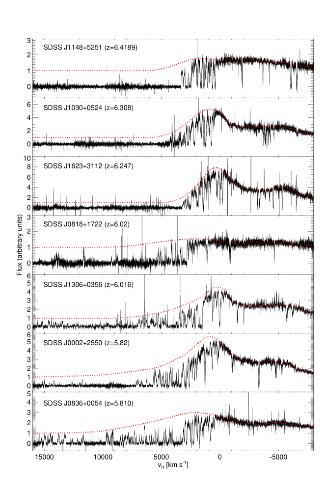
Figure 1: The seven quasar spectra analysed in this work against velocity with respect to the rest frame Ly$\alpha$ wavelength. The spectra have already been normalised by a power-law with $f_{\rm\nu}\propto\nu^{-0.5}$ (see text for details). A slowly varying spline (dotted red curves) has also been fitted to the Ly$\alpha$ emission lines in each spectrum to approximate the quasar continuum. A detailed analysis of the systematic uncertainty associated with the continuum fitting procedure is presented in Section 4.2.

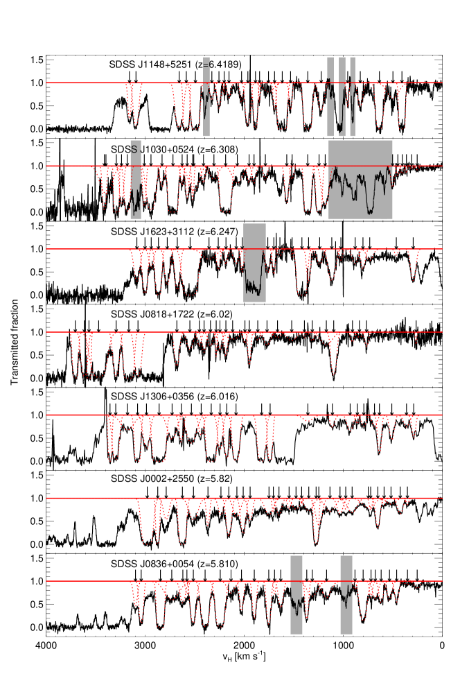
Figure 2: Transmitted fraction against the Hubble velocity blueward of the Ly$\alpha$ emission line for the seven quasar near-zones analysed in this work. The red dotted curves display the Voigt profile fits to the absorption lines made using VPFIT, with the centre of the lines marked by the downward pointing arrows. The grey shaded regions are identified as – or suspected of – containing metal lines, and are thus excluded from the analysis (see Section 4.1 for further details).

We analyse seven high-resolution quasar spectra in this work. The spectra for six of these objects were obtained using the High Resolution Echelle Spectrograph (HIRES, Vogt et al. 1994) on the 10-m Keck I telescope using a 0.86″slit, which produces a resolution of $R=40\,000$ (FWHM = $6.7\rm\,km\,s^{-1}$). The seventh spectrum was obtained using the Magellan Inamori Kyocera Echelle (MIKE, Bernstein et al. 2003) spectrograph on the 6.5-m Magellan II telescope. This instrument has a slightly lower resolution compared to HIRES, with FWHM=$13.6\rm\,km\,s^{-1}$. The data were processed using a custom set of IDL routines (Becker et al. 2006, 2007) that include optimal sky subtraction (Kelson 2003). The final binned pixel sizes are 2.1 km s^-1 for the HIRES spectra, and $5.0\rm\,km\,s^{-1}$ for the MIKE data.

The quasars are fully summarised in Table 1, and the spectra are displayed in Figures 1 and 2 . The systemic redshifts and absolute AB magnitudes are taken from Carilli et al. (2010). The continuum fitting in the near-zones was performed by first dividing the spectra by a power-law with $f_{\nu}\propto\nu^{-0.5}$, normalised near $1280\,(1+z)$ Å. The results of this procedure are displayed in Figure 1. The Ly$\alpha$ emission line was then fitted with a slowly varying spline, shown by the dotted red curves in Figure 1. The fully normalised near-zone spectra are displayed in Figure 2. Further details on the continuum fitting procedure may be found in B10, and the impact of the continuum fitting uncertainties on our results is examined in detail in Section 4.2.

We obtain the Doppler parameter CPDF for the Ly$\alpha$ absorption lines following a procedure identical to the approach described by B10. We use an automated version of the Voigt profile fitting package VPFIT, to fit lines over the velocity ranges indicated in Table 1. All lines with $\log(N_{\rm HI}/\rm cm^{-2})>17$, $b>100\rm\,km\,s^{-1}$ and with relative errors in excess of 50 per cent are discarded for the temperature analysis. These discarded lines make up 30 per cent of the total fitted to the data. The remaining line fits are indicated by the red dotted curves in Figure 2, with the centre of each line indicated by the downward pointing arrows. The resulting Doppler parameter CPDFs for each of the seven quasars are displayed in Figure 3.

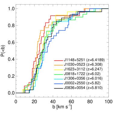
Figure 3: The Doppler parameter CPDFs obtained from the near-zones of the seven quasars analysed in this study. The Doppler parameters are obtained by fitting Voigt profiles to the Ly$\alpha$ absorption in the quasar near-zones, and exclude fits in regions suspected of containing metal absorption lines.

2.2 Hydrodynamical simulations

The synthetic Ly$\alpha$ absorption spectra used to calibrate the Doppler parameter CPDF measurements are constructed using high-resolution hydrodynamical simulations combined with a line-of-sight Lyman continuum radiative transfer algorithm. The hydrodynamical simulations were performed using the parallel Tree-SPH code GADGET-3, which is an updated version of the publicly available code GADGET-2 (Springel 2005). The simulations have a box size of $10h^{-1}$ comoving Mpc and a gas particle mass of $9.2\times 10^{4}h^{-1}M_{\odot}$. Outputs are obtained from the simulations at $z=6.42$, $z=6.28$, $z=6.01$ and $z=5.82$. Our procedure for constructing simulated quasar spectra along with the appropriate numerical convergence tests are discussed in detail by B10. For brevity, we focus instead on describing the additional improvements made for this study.

In order to explore the effect of a wide range of gas temperatures on the Doppler parameter CPDF, we perform an expanded set of hydrodynamical simulations which employ a variety of different thermal histories. We use 14 hydrodynamical simulations in total, which are summarised in Table 2. The initial gas temperature in these simulations, prior to any quasar heating, is set using a pre-computed ultra-violet (UV) background model. The fiducial UV background in this study is the galaxies and quasars emission model of Haardt & Madau (2001), in which the IGM is reionised instantaneously at $z=9$. In models A through to M, we construct simulations with different initial temperatures by rescaling the Haardt & Madau (2001) photo-heating rates with a constant factor, $\zeta$, such that $\epsilon_{\rm i}=\zeta\epsilon_{\rm i}^{\rm HM01}$. Here $\epsilon_{\rm i}^{\rm HM01}$ are the Haardt & Madau (2001) photo-heating rates for species $i=[\rm H\,\scriptstyle I$, $\rm He\,\scriptstyle I$, $\rm He\,\scriptstyle II$].

The temperature at mean density as a function of redshift in a selection of these hydrodynamical simulations, prior to any quasar heating, is displayed in Figure 4. The photo-heating is coupled to the hydrodynamical response of the gas in the simulations; different heating histories will therefore result in a different pressure smoothing scale for each model (e.g. Gnedin & Hui 1998; Pawlik et al. 2009). Since the Ly$\alpha$ line widths are sensitive to the changes in the gas temperature through Jeans smoothing in addition to thermal broadening (Peeples et al. 2010; Becker et al. 2011), we also consider two further customised UV background models, X and Y, for which photo-heating begins at $z=12$ and $z=15$, respectively. These models are displayed as the dotted and dashed curves in Figure 4. These extended heating histories will result in gas being pressure smoothed on larger scales, even if the instantaneous gas temperature is similar to our fiducial models. The models are chosen to provide a plausible upper limit to the Jeans smoothing scale at $z\simeq 6$, and we shall use them to explore the effect of uncertainties in the IGM thermal history on our results in Section 4.3.

2.3 Lyman continuum radiative transfer

We next include the impact of photo-heating by the quasar on the surrounding IGM using our line-of-sight radiative transfer algorithm. For each of the seven observed quasars, we first generate a set of synthetic lines-of-sight using the simulation output closest to the quasar systemic redshift. A total of 100 lines-of-sight of length $55h^{-1}$ comoving Mpc are extracted around the most massive haloes identified from each of the hydrodynamical simulations and for each quasar, yielding skewers through the IGM density, temperature and peculiar velocity field. For our fiducial thermal history, this yields a total of $1200$ simulated lines-of-sight for calibrating each of the seven observed Doppler parameter CPDFs.

The next stage is to compute the transfer of ionising radiation along the lines-of-sight. We assume the quasar spectra are described by a broken power law, $f_{\nu}\propto\nu^{-0.5}$ for $1050{\rm\,\AA}<\lambda<1450\,\rm\AA$ and $f_{\nu}\propto\nu^{-\alpha_{\rm q}}$ for $\lambda<1050\,\rm\AA$. We adopt a fiducial extreme-UV (EUV) spectral index of $\alpha_{\rm q}=1.5$ in this work, consistent with radio quiet quasars at lower redshift (e.g. Telfer et al. 2002). The optically bright phase of the quasars is assumed to be $t_{\rm q}=10^{7}\rm\,yr$ (Haehnelt et al. 1998; Croton 2009). We assume the H$\,\rm\scriptstyle I\$and He$\,\rm\scriptstyle I\$around the $z\simeq 6$ quasars is already highly ionised when the quasar turns on (e.g. Wyithe et al. 2008, B10), but that helium has yet to be doubly ionised. The subsequent reionisation and photo-heating of He$\,\rm\scriptstyle II\$by the quasar thus results in an additional IGM temperature increase of $7000$–$9000\rm\,K$. Note, however, an EUV spectral index which is softer (harder) than $\alpha_{\rm q}=1.5$ will decrease (increase) the amount of He$\,\rm\scriptstyle II\$photo-heating (Bolton et al. 2009; McQuinn et al. 2009). The IGM temperatures at mean density prior to and after He$\,\rm\scriptstyle II\$heating by the quasar are summarised in Table 2.

Table 2: The hydrodynamical simulations used in this work. From left to right, the columns list the simulation name, the scaling factor for the UVB photo-heating rates (see main text for details), the redshift which the gas is first photo-heated in the hydrodyamical simulations and the volume weighted gas temperature at mean density, both prior to and after He$\,\rm\scriptstyle II\$photo-heating by the quasar. The temperatures in this instance are shown for the simulations of SDSS J0818$+$1722 at $z=6.02$, but are broadly similar for the other six quasars.

Model	$\zeta$	$z_{\rm heat}$	$\log(T_{\rm 0}^{\rm initial}$/K)	$\log(T_{\rm 0}$/K)
A	0.1	9.0	3.29	4.03
B	0.3	9.0	3.62	4.11
C	0.5	9.0	3.78	4.16
D	0.8	9.0	3.93	4.22
E	1.1	9.0	4.02	4.27
F	1.8	9.0	4.17	4.35
G	2.6	9.0	4.28	4.42
H	3.6	9.0	4.37	4.49
J	4.7	9.0	4.45	4.54
K	5.9	9.0	4.51	4.59
L	7.8	9.0	4.59	4.65
M	9.3	9.0	4.63	4.69
X	Varied	12.0	4.00	4.26
Y	Varied	15.0	3.92	4.22

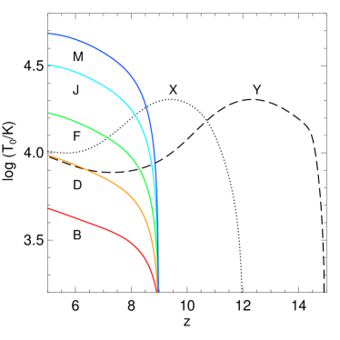
Figure 4: The temperature at mean density and its dependence on redshift for a selection of the hydrodynamical simulations listed in Table 2. The solid curves display the simulations using our fiducial thermal history which is based on the galaxies and quasars UV background of HM01. We also explore the effect of a more extended period of heating on our results with two additional models, X and Y. These are shown by the dotted and dashed curves, where the IGM is first heated at $z=12$ and $z=15$, respectively.

3 Methodology

We now briefly review our method for obtaining the near-zone temperature constraints from the Doppler parameter CPDF (but see B10 for further details). The advantage of using the Doppler parameter CPDF is that it fully uses the limited number of absorption lines available in the observational data and avoids the loss of information associated with binning. Although not all the absorption lines in the CPDF are purely thermally broadened (Theuns et al. 2000), the thermal broadening kernel nevertheless acts on all the Ly$\alpha$ absorption and the entire CPDF therefore remains sensitive to changes in the gas temperature. The second advantage is that we may compare the observed CPDFs to our simulations using the “D-statistic”, which is very similar to the parameter used in a Kolmogorov-Smirnov test (e.g. Press et al. 1992). This approach has the advantage of providing a non-parametric measure which quantifies the difference between Doppler parameter CPDFs drawn from different models and the data. On the other hand, obtaining absolute confidence intervals on the temperature using this method requires a large set of realistic simulations for calibrating the D-statistic, and these simulations are time consuming to perform and analyse.

For each quasar, we therefore use our sets of synthetic spectra to construct Monte Carlo realisations of the Doppler parameter CPDF for each of the fiducial simulations, A through to M. The simulated CPDFs are obtained by performing exactly the same line fitting procedure used on the observational data. For each simulated line-of-sight in the set of 100 spectra, we then measure the D-statistic, which is the maximum difference between the Doppler parameter CPDF for that simulated line-of-sight and the Doppler parameter CPDF for all 100 simulated lines-of-sight:

$$D_{\rm i}={\rm max}|P(<b)_{\rm i}-P(<b)_{\rm all}|,\,i=1...100,$$ (1)

where we preserve the sign of the difference. The D-statistic CPDF for a model with known temperature $\log T_{0}$, $P(<D|\log T_{0})$, can then be constructed. We then smooth over the noise arising from the discrete sampling of the D-statistic CPDF with a Gaussian filter of width $\sigma=0.025$ before computing its derivative, $\frac{dP(<D_{\rm obs}|\log T_{0})}{dD}$. Note that in this work we fit 100 spectra for each model, as opposed to only 30 in B10, enabling a finer sampling of the D-statistic distribution.

By then measuring the D-statistic for the observed line-of-sight, $D_{\rm obs}$, we may then use the D-statistic CPDF along with Bayes’ theorem to obtain a probability distribution for the logarithm of the observed temperature at mean density, $\log T_{0}$:

$$p(\log T_{0}|D_{\rm obs})=K\frac{dP(<D_{\rm obs}|\log T_{0})}{dD}p(\log T_{0}),$$ (2)

where $p(\log T_{0})$ is the prior on $\log T_{0}$ and $K$ is a constant which normalises the total probability to unity. As in B10, we adopt a flat prior, $p(\log T_{0})$, but adopt a more extended prior temperature range, $3.2\leq\log(T_{0}/\rm K)\leq 4.8$ using our expanded set of simulations. The prior is chosen to encompass the range of full range of initial and final temperatures in our simulations (see Table 2) and is intended to represent a reasonable range for the IGM temperature following He$\,\rm\scriptstyle II\$and/or H$\,\rm\scriptstyle I\$reionisation (see e.g. Trac et al. 2008; McQuinn et al. 2009). We then evaluate $\frac{dP(<D_{\rm obs}|\log T_{0})}{dD}$ at twelve discrete points using each of our fiducial hydrodynamical simulations, and use a cubic spline to interpolate between these to obtain a continuous distribution. Lastly, we infer confidence intervals around the median $\log T_{0}$ by integrating $p(\log T_{0}|D_{\rm obs})$ over the appropriate limits. All our temperature measurements are therefore quoted as the median of the $p(\log T_{0}|D_{\rm obs})$ distribution with the confidence intervals around the median. This will be implicit throughout the remainder of the paper.

4 Systematic uncertainties

We now turn to examine the key systematic uncertainties in our analysis. In B10, we considered five potential sources of systematic error. The first three – the mean transmitted fraction in the quasar near-zone, the influence of strong galactic winds, and the dependence of the IGM temperature on gas density, were found to have a negligible effect on the Doppler parameter CPDF. In the latter case, this is because transmission in the $z\simeq 6$ near-zones is sensitive to gas close to mean density. On the other hand, B10 estimated that metal line contamination and uncertainties in the continuum placement could systematically bias temperature measurements by up to $\sim 2000\rm\,K$. Although these uncertainties are small compared to the statistical uncertainty on the B10 measurement for a single line-of-sight, they will be important to consider for the larger data set used in this study. We furthermore examine an additional and important systematic which was not included in B10 – the effect of the uncertain thermal history at $z>6$ (e.g. Becker et al. 2011).

4.1 Metal lines

We first examine the effect of metal line contamination on our results. As our synthetic spectra do not include absorption from intervening metals, we must remove any metal contamination present in the observational data in order to avoid biasing our temperature measurements. The erroneous identification of metal lines as H$\,\rm\scriptstyle I\$Ly$\alpha$ absorption can lead to underestimated temperatures, since in general metal ions exhibit significantly narrower line widths compared to the Ly$\alpha$ lines.

Our approach is to identify possible metal lines in the quasar near-zones and exclude these regions from our Doppler parameter analysis. Potential contaminants lying within the near-zones were first identified by searching for metal line systems at other wavelengths in the quasar spectra, and flagging any associated lines within the near-zones. This was followed by flagging any absorption features in the near-zones that subsequently remained unidentified and appeared too narrow to be H$\,\rm\scriptstyle I\$Ly$\alpha$ lines. This procedure is most reliable for quasars which have near-IR spectra, enabling greater coverage redward of the Ly$\alpha$ emission line. Near-IR data was available for five of the seven quasars analysed in this work; the exceptions are J1623$+$3112 and J1306$+$0356.

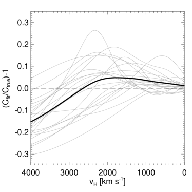
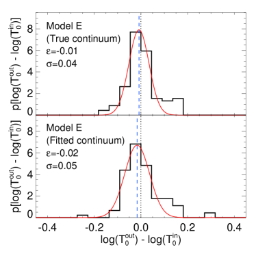
Figure 5: Left: The continuum level, $C_{\rm fit}$, recovered from a blind analysis of $20$ synthetic spectra relative to the true unabsorbed continuum, $C_{\rm true}$, against Hubble velocity blueward of rest-frame Ly$\alpha$. The light grey curves display the relative continuum uncertainty for each spectrum, while the thick black line shows the average. Upper right: The distribution of the difference between the temperature recovered using the algorithm detailed in Section 3 and the input value, $\log T_{0}^{\rm out}-\log T_{0}^{\rm in}$ (black solid lines), for 100 synthetic spectra drawn from model E where the true continuum is known exactly. The resulting distribution may be approximated by a Gaussian with mean $\epsilon=-0.01$ dex and standard deviation $\sigma=0.04$ dex (red solid curve), indicating that the true temperature is recovered well with some intrinsic scatter. The vertical black dotted line and blue dashed lines mark the zero offset and mean of the best fit Gaussian, respectively. Lower right: The distribution of $\log T_{0}^{\rm out}-\log T_{0}^{\rm in}$ for the same spectra after randomly dividing each by one of the error functions in the left-hand panel. The distribution may be approximated as a Gaussian with an offset of $\epsilon=-0.02$ dex and standard deviation $\sigma=0.05$ dex.

The contaminated regions identified in the near-zones are marked by the grey shaded regions in Figure 2, and are excluded from our Doppler parameter CPDF analysis. For three of the quasars, J0818$+$1722, J1306$+$0356 and J0002$+$2550, no metal lines were identified. Removing the metal contamination slightly raises the temperature constraints obtained from the other four spectra, producing an increase of $\sim 0.02$ dex in our $\log T_{0}$ constraints. Note, however, that it is possible that metal lines which are highly blended with the Ly$\alpha$ lines remain unidentified. Throughout the rest of the paper, we therefore conservatively add an additional scatter of $0.02$ dex in quadrature to our final $\log T_{0}$ constraints for each line-of-sight.

4.2 Continuum placement

The second important systematic identified in B10 was the effect of continuum placement uncertainties on the temperature measurements. If the continuum is placed too low (high) on the observational data, the IGM temperature around the quasars will be underestimated (overestimated) as the absorption line widths are effectively narrowed (broadened). B10 attempted to account for continuum placement uncertainties by normalising the synthetic spectra by the highest transmitted flux in segments of length $1000\rm\,km\,s^{-1}$. The motivation for this was to minimise bias by treating the synthetic data in a similar fashion to the observational data.

However, the drawback of this approach is that it only crudely mimics the continuum fitting process on the observational data. In this study, we instead perform “blind” normalisations on the synthetic spectra to estimate the continuum placement uncertainty (see also e.g. Tytler et al. 2004; Faucher-Giguère et al. 2008). Our procedure is as follows. One of us (JSB) constructed $20$ different simulated spectra with sufficient wavelength coverage on either side of the Ly$\alpha$ emission line for normalisation. Each spectrum was then multiplied with one of the continuum fits compiled by Kramer & Haiman (2009), obtained from a large sample of low redshift, unobscured quasars. The spectra were then processed to resemble the resolution and noise properties of the quasars analysed in this work. A second author (GDB), who was responsible for continuum fitting the observational data, then proceeded to normalise the synthetic spectra without any prior knowledge of the true continuum.

The results of the blind continuum fits to the synthetic data are displayed in the left panel of Figure  5, where the continuum level, $C_{\rm fit}$, recovered from the analysis is shown relative to the true continuum, $C_{\rm true}$, against Hubble velocity blueward of rest frame Ly$\alpha$. The light grey curves display the relative continuum uncertainty for each of the 20 synthetic spectra, while the thick black line shows the average. On average the continuum is placed to within 5 per cent of the true value within $\sim 3000\rm\,km\,s^{-1}$ of the quasar redshift, where the uncertain shape of the quasar Ly-$\alpha$ emission line is the largest uncertainty. However, the continuum placement is almost always biased low beyond $>3000\rm\,km\,s^{-1}$ – by as much as 15 per cent on average – where the transmitted flux rarely recovers to the unabsorbed level. Fortunately, since the majority of the absorption lines fitted to the observational data in this work lie within $3000\rm\,km\,s^{-1}$ of the quasar systemic redshift, this suggests that the impact of the continuum placement on our temperature measurements should be relatively modest.

We quantify this in the right-hand panel of Figure 5, where the recovery of the IGM temperature at mean density from the simulated Doppler parameter CPDF is tested. The upper panel displays the distribution of the difference between the input temperature, $\log T_{0}^{\rm in}$, and the recovered temperature, $\log T_{0}^{\rm out}$, for 100 simulated spectra drawn from model E. This distribution may be approximated by a Gaussian, displayed by the red curve. In this instance the continuum is assumed to be known exactly, and the input temperature is recovered accurately (to within $0.01$ dex, with a small scatter of $\sim 0.04$ dex).

For comparison, in the lower right hand panel of Figure 5 we display the distribution of $\log T_{0}^{\rm out}-\log T_{0}^{\rm in}$ for the same spectra, but after they have been divided at random by one of the error functions displayed in the left hand panel of Figure 5. It is apparent that the temperature recovery is only very mildly impacted by the continuum placement. The recovered temperatures are biased to slightly lower temperatures (by $0.02$ dex) with some additional scatter. This is a smaller effect than that predicted by B10, who estimated the continuum fitting process could bias the temperature measurements by as much as $\sim 2000\rm\,K$. In order to test this further, we therefore also performed the same temperature recovery test on a set of spectra drawn from model E, but this time using the normalisation procedure used by B10. This resulted in temperatures which were biased low by $0.03$ dex. This suggests that the approximate method used in B10 slightly over-compensates for the relatively modest systematic offset in the recovered temperature due to continuum placement.

We therefore conclude that the uncertain continuum placement will introduce only a small additional uncertainty to our results. Nevertheless, we shift all our temperature measurements upward by $+0.02$ dex to account for the estimated continuum bias, and a further $0.03$ dex is added in quadrature to our estimated uncertainties for each line-of-sight.

4.3 Jeans smoothing and the thermal history

The third and final systematic we examine is the uncertain thermal history of the IGM at $z>6$. This will impact on the small-scale structure of the Ly$\alpha$ forest at $z\simeq 6$ through the effect of Jeans smoothing (e.g. Gnedin & Hui 1998; Pawlik et al. 2009). The finite amount of time required for gas pressure to respond to changes in the temperature means that two models with different thermal histories will be pressure smoothed on different scales, even if the instantaneous temperature is similar at the quasar redshift. In practice, because we rely on the simulations to calibrate the relationship between the Doppler parameter CPDF and the IGM temperature, if the true thermal history of the IGM is different to that assumed in our models, a systematic bias will be imparted to our measurements. Unfortunately, since the IGM temperature is unconstrained at $z>6$, the thermal history introduces an important uncertainty into our analysis (e.g. Becker et al. 2011).

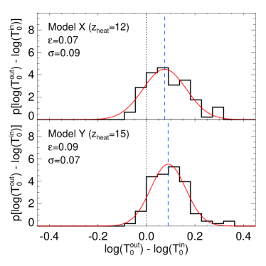
Figure 6: The effect of the uncertain IGM thermal history at $z>6$ on the temperatures recovered from quasar near-zones. Top: The distribution of the offset in the recovered temperature from the input value, $\log T_{0}^{\rm out}-\log T_{0}^{\rm in}$ (black solid lines), for 100 synthetic spectra drawn from Model X, in which photo-heating of the IGM begins at $z=12$. Bottom: The distribution for model Y, with heating beginning at $z=15$. In both panels, the red curves show the best-fit Gaussian, with mean $\epsilon$ and standard deviation $\sigma$ indicated on the panels, while the vertical black dotted line and blue dashed lines mark the zero offset and the mean of the best-fit Gaussian, respectively.

We investigate the impact of the uncertain thermal history on our results in Figure 6, where we examine the accuracy with which temperatures are recovered from spectra drawn from models X and Y. These models have thermal histories which are more extended than our fiducial models, with heating beginning at $z=12$ and $z=15$, respectively (see Figure 4). The increased amount of early heating in these two models means that the IGM has had longer to dynamically respond to the increased temperatures. As a result, the gas distribution in these models is physically smoothed on a larger scale. In practice, this means that relative to our fiducial simulations, a greater proportion of the line broadening in spectra constructed from these simulations will be due the increased physical extent of the absorbers rather than Doppler broadening.

As a consequence, the recovered distributions for $\log T_{0}^{\rm out}-\log T_{0}^{\rm in}$ in Figure 6 demonstrate that the inferred temperatures for models X and Y are significantly higher, by $0.07$–$0.09$ dex, compared to the true temperature in the models. The measurements also exhibit more scatter ($\sigma\sim 0.07$–$0.09$ dex) around the mean than observed for the fiducial models (e.g. the upper right panel in Figure 5). As might be expected, the systematic offset in the recovered temperature is slightly larger for the model where heating begins at $z=15$. The very uncertain thermal history $z>6$ therefore means it is possible that we may overestimate the IGM temperature in the real quasar near-zones by as much as $0.1$ dex. On the other hand, if reionisation occurred very late we may underestimate the temperatures. However, the latter case will make our conclusions regarding He$\,\rm\scriptstyle II\$photo-heating around the quasars stronger, rather than weaker. We therefore address this issue in the next section by presenting temperature measurements which include an estimate of the impact of additional Jeans smoothing along with our fiducial results. These Jeans smoothing related uncertainties are estimated based on the results of this analysis: we correct for a systematic offset by shifting our constraints by $-0.08$ dex and adding an additional scatter of $\sigma=0.07$ dex in quadrature to the measurement uncertainties for each line-of-sight.

5 Results

5.1 Line-of-sight temperature constraints

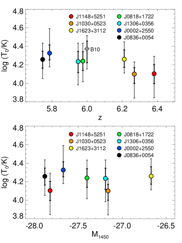
Figure 7: Upper panel: The filled circles display the recovered near-zone temperatures at mean density against redshift for the seven quasar spectra analysed in this work. The thick (thin) error bars show the 68 (95) confidence intervals. The data points for J1306$+$0356 and J0836$+$0054 have been offset by $\Delta z=-0.03$ for clarity. The grey diamond compares the measurement for J0818$+$1722 obtained by B10. Lower panel: The near-zone temperature at mean density against quasar absolute magnitude at $1450\rm\,\AA$.

We now present the main results of this study by first considering the temperature measurements obtained for the individual lines-of-sight. The temperature measurements at mean density derived for our fiducial thermal history are summarised in Table 3, and are plotted as a function of redshift (upper panel) and quasar absolute magnitude (lower panel) in Figure 7. It is reassuring to note that the temperature constraints mirror the Doppler parameter CPDFs displayed in Figure 3, with the lowest temperatures derived from the CPDFs with the smallest Doppler parameters on average. The two highest redshift quasars, J1148$+$5251 and J1030$+$0524, exhibit slightly lower temperatures compared to the rest of the sample, while on the other hand J0002$+$2550 has a slightly higher temperature. However, the measurement uncertainties are such that all seven quasars are consistent with the same IGM temperature within the 95 per cent confidence intervals.

In the upper panel of Figure 7, the temperature constraints are also compared to the measurement for J0818$+$1722 presented by B10, shown by the grey diamond. Although our revised measurement for J0818$+$1722 is formally consistent within the 68 per cent confidence interval, it is systematically lower by $\sim 0.13$ dex. The first reason for this difference is that in B10 the redshift of J0818+1722 was given as $z=6.00$ (Fan et al. 2006). The revised redshift of $z=6.02$ presented by Carilli et al. (2010) now extends the region where we fit absorption lines by $855\rm\,km\,s^{-1}$, resulting in an additional five absorption lines in the near-zone (yielding a total of 30). These lines lower the median Doppler parameter by $\sim 1.7\rm\,km\,s^{-1}$, and shift the temperature constraint downward by $\sim 0.03$ dex. The second difference is our improved treatment of the continuum uncertainty. As discussed in Section 4.2, the approximate continuum uncertainty correction used in B10 produces temperatures which are $\sim 0.01$ dex higher compared to our new results. The third difference is the extended prior probability used in this work, especially at lower temperatures. We may approximate the B10 measurements by using only models C to J for our analysis and restricting the prior probability to $4.13\leq\log(T_{0}/\rm K)\leq 4.56$. This yields a temperature $\sim 0.03$ dex higher than the value obtained using the full simulation set.

5.2 Average temperature constraints

The primary improvement of this study is the enlarged sample of seven quasars at $z\simeq 6$, which enables us to significantly improve upon the large statistical uncertainty in the individual line-of-sight measurement presented by B10. The average temperature constraints derived from the Doppler parameter CPDF for all seven quasars are therefore given in the final two rows of Table 3. As discussed in Section 4.3, each column gives the measurements for both our fiducial thermal history and the case of additional Jeans smoothing arising from a more extended heating history.

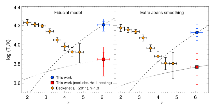
Figure 8: Left: The filled blue circle shows the temperature at mean density recovered from all seven quasar spectra analysed in this work. The thick (thin) error bars display the the 68 (95) per cent confidence intervals. The red square shows the temperature constraint after subtracting the expected photo-heating from the reionisation of He$\,\rm\scriptstyle II\$by the quasars. For comparison, the open diamonds give the temperature measurements from the general Ly$\alpha$ forest at $z<5$ obtained by Becker et al. (2011) with $2\sigma$ uncertainties. The slope for the IGM temperature-density relation, $T=T_{0}(1+\delta)^{\gamma-1}$, is assumed to be $\gamma=1.3$. The dashed curve shows the expected redshift evolution if the IGM cools adiabatically, $T_{0}\propto(1+z)^{2}$, while the dotted curve follows the thermal asymptote, $T_{0}\propto(1+z)^{0.53}$. These curves approximate the maximum and minimum rate of cooling expected toward lower redshift. Right: As for the left panel, except now the near-zone temperature constraints are adjusted for the possible systematic due to additional Jeans smoothing (see Section 4.3 for details). Following Becker et al. (2011), the $z<5$ measurements have also been shifted downward by $2000\rm\,K$, reflecting the expected systematic shift these authors find at $z\simeq 4$-5 when including additional Jeans smoothing in their analysis.

The average measurements for all seven quasar are displayed in Figure 8, where they are also compared to the IGM temperature measurements at $z<5$ presented recently by Becker et al. (2011). The left hand panel displays the measurements obtained using our fiducial thermal history, while the right hand panel shows our constraints after accounting for additional Jeans smoothing. Note that the Becker et al. (2011) measurements in the right panel have been shifted downward by $2000\rm\,K$, reflecting the approximate expected systematic shift these authors find at $z\simeq 4$-5 when including additional Jeans smoothing in their analysis.

In each panel, we furthermore show two different versions of our $z\simeq 6$ temperature measurements. The blue circle shows the temperature constraint obtained directly from the Doppler parameter CPDF for all seven lines-of-sight. In addition, the red square shows the constraint on the initial temperature of the IGM before the quasars reionise the He$\,\rm\scriptstyle II\$in their vicinity. Here we have used the He$\,\rm\scriptstyle II\$heating estimates from our radiative transfer simulations to remove the contribution of the in-situ He$\,\rm\scriptstyle II\$photo-heating by the quasars. In practice, this is achieved by evaluating Eq. (2) using the initial IGM temperature, $T_{0}^{\rm initial}$, in our models rather than the temperature after He$\,\rm\scriptstyle II\$heating by the quasar. Note that this constraint assumes the average quasar EUV spectral index is $\alpha_{\rm q}=1.5$; a harder (softer) spectral index would lower (raise) these constraints. The advantage of these measurements is that they attempt to remove the impact of He$\,\rm\scriptstyle II\$heating by the quasar, and should therefore more closely represent the temperature of the general IGM prior to He$\,\rm\scriptstyle II\$reionisation. These constraints may therefore be more easily compared to expectations for the thermal state of the IGM following H$\,\rm\scriptstyle I\$reionisation (Furlanetto & Oh 2009; Cen et al. 2009).

We qualitatively explore the implications of these measurements for reionisation and the IGM thermal history using two simple evolutionary models for the IGM temperature, shown by the dashed and dotted curves in Figure 8. The dashed line, which scales as $T_{0}\propto(1+z)^{2}$, is normalised to match our temperature constraint including He$\,\rm\scriptstyle II\$heating. This curve represents the maximum possible (adiabatic) cooling rate toward lower redshift in the absence of any additional heating. In contrast, the dotted curve scales as $T_{0}\propto(1+z)^{0.53}$ and is normalised to pass through the constraint with He$\,\rm\scriptstyle II\$heating subtracted. This curve approximates the minimum amount of cooling expected if the IGM temperature is asymptotically approaching the thermal state set by the spectral shape of the UV background (Hui & Haiman 2003).

Although the absolute values for the temperatures are lower when including additional Jeans smoothing, the general conclusions we draw from the relative values of the temperature data remain the same regardless of the uncertain thermal history at $z>6$. The results in Figure 8 imply that (i) there is an additional and significant source of heating around the $z\simeq 6$ quasars which is not yet present in the general IGM at $z\simeq 5$ and (ii) there is evidence for a constant or gradually increasing temperature in the general IGM from $z\simeq 6$ to $z\simeq 5$. The first point suggests that we may be observing evidence for the earliest stages of He$\,\rm\scriptstyle II\$reionisation in the immediate environment of these high redshift quasars. The second point agrees with the suggestion by Becker et al. (2011) that there is a gradual increase in the temperature of the general IGM at $z<5$ due to the impact of an extended epoch of He$\,\rm\scriptstyle II\$reionisation globally (but see also the suggestion by Chang et al. 2011 that significant additional heating at $z<5$ may arise from TeV blazars, assuming the kinetic energy of ultra-relativistic pairs is converted to thermal energy via plasma beam instabilities).

Table 3: The temperature measurements obtained from the Doppler parameter CPDF in the near-zones of the seven quasars analysed in this study. From left to right, each column lists the quasar name, the redshift range over which the Doppler parameters were measured from the spectrum, and the final constraints for our fiducial thermal history and for the case of the additional Jeans smoothing expected from a very extended period of heating at $z>6$ (see Section 4.3 for details). The final two rows also show the line-of-sight averaged constraints obtained for all seven quasars, with the last row giving the temperature measurement after subtracting the expected heating from the local reionisation of He$\,\rm\scriptstyle II\$by the quasar. In all instances we assume a flat prior probability of $3.2\leq\log(T_{0}/\rm K)\leq 4.8$.

Quasar	$z$	log ($T_{0}$/K)	log ($T_{0}$/K)
		(Fiducial)	(Extra Jeans smoothing)
SDSS J1148$+$5251	$6.38\pm 0.03$	$4.10^{+0.10}_{-0.11}$ (${}^{+0.19}_{-0.26}$)	$4.02^{+0.12}_{-0.13}$ (${}^{+0.23}_{-0.29}$)
SDSS J1030$+$0524	$6.27\pm 0.04$	$4.10^{+0.07}_{-0.10}$ (${}^{+0.13}_{-0.26}$)	$4.01^{+0.10}_{-0.12}$ (${}^{+0.20}_{-0.28}$)
SDSS J1623$+$3112	$6.21\pm 0.03$	$4.26^{+0.10}_{-0.09}$ (${}^{+0.19}_{-0.15}$)	$4.18^{+0.12}_{-0.11}$ (${}^{+0.23}_{-0.21}$)
SDSS J0818$+$1722	$5.98\pm 0.04$	$4.24^{+0.10}_{-0.10}$ (${}^{+0.19}_{-0.22}$)	$4.16^{+0.12}_{-0.12}$ (${}^{+0.25}_{-0.26}$)
SDSS J1306$+$0356	$5.98\pm 0.03$	$4.24^{+0.11}_{-0.12}$ (${}^{+0.20}_{-0.25}$)	$4.15^{+0.13}_{-0.14}$ (${}^{+0.25}_{-0.29}$)
SDSS J0002$+$2550	$5.79\pm 0.03$	$4.33^{+0.09}_{-0.07}$ (${}^{+0.27}_{-0.15}$)	$4.25^{+0.12}_{-0.10}$ (${}^{+0.28}_{-0.21}$)
SDSS J0836$+$0054	$5.78\pm 0.03$	$4.26^{+0.09}_{-0.09}$ (${}^{+0.18}_{-0.21}$)	$4.18^{+0.11}_{-0.12}$ (${}^{+0.23}_{-0.25}$)
All	$6.08\pm 0.33$	$4.21^{+0.03}_{-0.03}$ (${}^{+0.06}_{-0.07}$)	$4.13^{+0.04}_{-0.04}$ (${}^{+0.08}_{-0.08}$)
All (He$\,\rm\scriptstyle II\$heating subtracted)	$6.08\pm 0.33$	$3.85^{+0.08}_{-0.08}$ (${}^{+0.13}_{-0.17}$)	$3.77^{+0.08}_{-0.09}$ (${}^{+0.14}_{-0.18}$)

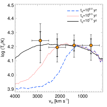
Figure 9: The temperature at mean density as a function of Hubble velocity blueward of the quasar Ly$\alpha$ emission lines. The data points are derived from all seven quasars in our sample, where the thick (thin) error bars represent the 68 (95) per cent confidence intervals. The solid black, dotted red and dashed blue curves show the temperature at mean density predicted by radiative transfer simulations constructed from model D for an optically bright phase of $t_{\rm q}=10^{7}$, $10^{6.5}$ and $10^{6}$ yr respectively. Assuming the quasars reionised He$\,\rm\scriptstyle II\$in their environment, a flat thermal profile is inconsistent with an optically bright phase of duration $t_{\rm q}\leq 10^{6.5}\rm\,yr$.

5.3 The thermal proximity effect

Finally, as we suspect these quasars may have recently reionised the He$\,\rm\scriptstyle II\$in their vicinity, it is interesting to also examine the IGM temperature as a function of distance from the quasars. We therefore now consider the possibility of directly observing the line-of-sight “thermal proximity effect”, which will arise from the elevated temperatures expected in the He$\,\rm\scriptstyle III\$regions created by these quasars (Miralda-Escudé & Rees 1994; Theuns et al. 2002b; Meiksin et al. 2010).

Assuming the optically bright phase of a quasar is significantly shorter than the recombination timescale, $t_{\rm q}\ll t_{\rm rec}^{\rm HeIII}$, the typical size of a quasar He$\,\rm\scriptstyle III\$region in proper Mpc is

$$R_{\rm HeIII}\simeq 5.5{\rm\,Mpc}\left(\frac{{\dot{N}}_{56}}{3.5}\right)^{1/3}\left(\frac{t_{\rm q}}{10^{7}\rm\,yr}\right)^{1/3}\left(\frac{1+z}{7}\right)^{-1/3}.$$ (3)

Here ${\dot{N}}_{56}={\dot{N}}_{\rm HeII}/10^{56}\rm\,s^{-1}$ is the number of He$\,\rm\scriptstyle II\$ionising photons emitted per second, which for the quasars analysed in this work ranges from ${\dot{N}}_{56}\simeq 1.7$–$5.3$ assuming an EUV spectral index of $\alpha_{\rm q}=1.5$. A thermal proximity effect will thus be detectable only if the quasar He$\,\rm\scriptstyle III\$regions are on average smaller than the scales over which we make our temperature measurements ($\sim 5$ proper Mpc). Note also that the adiabatic cooling timescale, which is the appropriate cooling rate for gas at mean density expanding with the Hubble flow, is $t_{\rm ad}\simeq 1/2H(z)=7.2\times 10^{8}\rm\,yr$ at $z=6$ (cf. the age of the Universe at $z=6$, $t_{\rm age}\simeq 9.6\times 10^{8}\rm\,yr$). Consequently, the thermal proximity effect should provide a reasonable constraint on the total duration of the optically bright lifetime for these quasars. We may therefore infer from Eq. (3) that the detection of significantly lower temperatures at the edge of the quasar near-zones would imply a rather short optically bright phase on average for these objects, $t_{\rm q}<10^{7}\rm\,yr$.

We obtain the radial temperature measurements by splitting the absorption line fits from all seven quasars into four bins of width $750\rm\,km\,s^{-1}$ over the range $250\rm\,km\,s^{-1}\leq v_{\rm H}\leq 3250\rm\,km\,s^{-1}$. We then use the Doppler parameter CPDF in each of the four bins to obtain temperature measurements at mean density in the usual manner. Note that due to the small number of lines in each bin for individual quasars (typically $6-8$), it is not possible to obtain useful constraints from each quasar individually.

The results of this procedure are displayed as the data points with error bars in Figure 9, and are consistent with constant temperature of $\log(T_{0}/\rm K)\sim 4.2$ within $\sim 3250\rm\,km\,s^{-1}$ of these quasars. These are compared to a selection of radial temperature profiles from our line-of-sight radiative transfer calculations. The simulations are constructed using model D, with an initial temperature of $\log(T_{0}/\rm K)\sim 3.9$, and are identical to the models used to construct our synthetic spectra with the exception that we also now consider two shorter optically bright phases of $t_{\rm q}=10^{6.5}\rm\,yr$ and $t_{\rm q}=10^{6}\rm\,yr$. The temperature profiles displayed are averaged over all 100 simulated lines-of-sight and smoothed by a box car window of width $100\rm\,km\,s^{-1}$ for clarity. It is evident from this simple comparison that, under the assumption the quasars have reionised the He$\,\rm\scriptstyle II\$in their vicinity, the data are inconsistent with an optically bright phase with $t_{\rm q}<10^{6.5}\rm\,yr$. However, due to the relatively restricted range probed by the near-zones we are unable to detect clear evidence for a thermal proximity effect.

Future progress in this area may be possible at slightly lower redshift, where line widths can be analysed at larger distances from the quasar. However, detecting the thermal proximity effect in quasar spectra at $z<3$ will likely difficult, since it is expected He$\,\rm\scriptstyle II\$reionisation is largely complete by this time (e.g. Shull et al. 2010; Worseck et al. 2011). Analyses at slightly higher redshift, $z>3.5$, may therefore be best placed for such a study. On the other hand, a recent theoretical study by Meiksin et al. (2010) found that peculiar motions and IGM density variations can result in the Ly$\alpha$ line widths exhibiting very little dependence on the distance from the quasar, even in the presence of a thermal proximity effect. Detailed simulations which correctly model the IGM density and velocity field will therefore be required to extract temperature measurements from the data.

6 Conclusions

In this work we present improved measurements of the temperature of the IGM at mean density around $z\simeq 6$ quasars. We use a sample of seven high-resolution quasar spectra, combined with detailed simulations of the thermal state of the inhomogeneous IGM, to improve upon the first direct measurement of the IGM temperature around J0818$+1$722 at $z\simeq 6$ presented by B10. This study therefore builds upon the work of B10 in three important ways, by using a larger sample of quasars, an expanded set of numerical simulations for calibrating the temperature measurements, and a more detailed analysis of systematic uncertainties. We find that the most important systematic is the thermal history of the IGM at $z>6$, which impacts on our measurements through the uncertain contribution of Jeans smoothing to the widths of Ly$\alpha$ absorption lines.

The temperature at mean density averaged over all seven lines-of-sight is $\log(T_{0}/\rm K)=4.21\pm^{0.03}_{0.03}$ ($\pm^{0.06}_{0.07}$) at 68 (95) per cent confidence. On comparison to constraints on the temperature of the general IGM at $z\sim 4.8$ which are consistent with $\log(T_{0}/\rm K)=3.9\pm 0.1$ within $2\sigma$, these data suggest that there is an additional and significant source of heating around the $z\simeq 6$ quasars which is not yet present in the general IGM at $z\simeq 5$. This is most likely due to the recent reionisation of He$\,\rm\scriptstyle II\$in the vicinity of these quasars, which is driven by their hard non-thermal ionising spectra. The elevated temperatures may therefore represent the first stages of He$\,\rm\scriptstyle II\$reionisation in the most biased locations in the high redshift Universe. It is furthermore found that when subtracting the expected amount of He$\,\rm\scriptstyle II\$photo-heating from the quasars, and assuming a canonical EUV spectral index of $\alpha_{\rm q}=1.5$, the general IGM temperature is similar to that measured at $z\simeq 4.8$. This agrees with the suggestion by Becker et al. (2011) that the observed rise in the IGM temperature at $z\leq 4.4$ is consistent with the onset of an extended epoch of He$\,\rm\scriptstyle II\$reionisation globally.

We also examine the evidence for a line-of-sight thermal proximity effect around these quasars by analysing the Doppler parameters for all seven lines-of-sight in radially spaced bins. We find no clear evidence for a thermal proximity effect due to an He$\,\rm\scriptstyle III\$region around the quasar, but note that the limited extent of the near-zone prevents us from detecting photo-heated He$\,\rm\scriptstyle III\$bubbles larger than $\sim 5$ proper Mpc in size. Under the assumption that the quasar has reionised the He$\,\rm\scriptstyle II\$in its vicinity, the data are therefore inconsistent with a short optically bright phase $t_{\rm q}<10^{6.5}\rm\,yr$.

Finally, in this work we have not examined the implications of our temperature measurements for H$\,\rm\scriptstyle I\$reionisation at $z>6$. These high-redshift temperature measurements should still probe the thermal signature of this landmark event, potentially yielding valuable insights into the timing and duration of this process (e.g. Theuns et al. 2002a; Hui & Haiman 2003; Furlanetto & Oh 2009; Trac et al. 2008; Cen et al. 2009). We intend examine this in detail in future work.

Appendix A Tests of the temperature measurement procedure

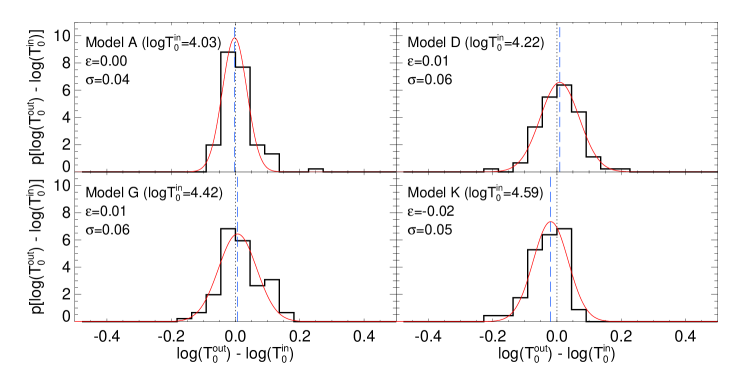
Figure 10: In each panel the distribution of the difference between the temperature at mean density measured from 100 synthetic near-zone spectra and the input value, $\log T_{0}^{\rm out}-\log T_{0}^{\rm in}$, is displayed by the solid black lines. The red solid curves display the best fit Gaussian to the distribution, and the vertical black dotted and dashed blue lines mark the zero offset and the mean of the best fit Gaussian, respectively. Upper left: The $\log T_{0}^{\rm out}-\log T_{0}^{\rm in}$ distribution for Model A, with a best fit Gaussian with mean $\epsilon=0.00$ dex and standard deviation $\sigma=0.04$ dex. Upper right: Model D, $\epsilon=+0.01$ dex, $\sigma=0.06$ dex. Lower left: Model G, $\epsilon=+0.01$ dex, $\sigma=0.06$ dex. Lower right: Model K, $\epsilon=-0.02$ dex, $\sigma=0.05$ dex.

Tests of the temperature measurement procedure described in Section 3 are displayed in Figure 10. The solid black lines show distributions of the difference between the temperature at mean density measured from 100 synthetic spectra and the input value, $\log T_{0}^{\rm out}-\log T_{0}^{\rm in}$, for four of our fiducial models. The models span a temperature range consistent with the observational measurements presented in this work. The distributions may be approximated by a Gaussian with mean $\epsilon$ and standard deviation $\sigma$, shown by the solid red curves. The means are within $\leq 0.02$ dex of the true input temperature in all cases, indicating our temperature measurement procedure is reliable to this level in the absence of any additional systematic uncertainties. Note, however, the accuracy of the temperature recovery is slightly poorer for model K, where the distribution is skewed to lower temperatures. This will be true in general for models with progressively higher temperatures; the line widths scale as the square root of the temperature, $b\propto T^{1/2}$, and the Doppler parameter CPDF thus has less discriminative power as the temperature increases.

References

- Becker et al. (2011) Becker, G. D., Bolton, J. S., Haehnelt, M. G., & Sargent, W. L. W. 2011, MNRAS, 410, 1096
- Becker et al. (2007) Becker, G. D., Rauch, M., & Sargent, W. L. W. 2007, ApJ, 662, 72
- Becker et al. (2006) Becker, G. D., Sargent, W. L. W., Rauch, M., & Simcoe, R. A. 2006, ApJ, 640, 69
- Bernstein et al. (2003) Bernstein, R., Shectman, S. A., Gunnels, S. M., Mochnacki, S., & Athey, A. E. 2003, in Society of Photo-Optical Instrumentation Engineers (SPIE) Conference Series, Vol. 4841, Society of Photo-Optical Instrumentation Engineers (SPIE) Conference Series, ed. M. Iye & A. F. M. Moorwood, 1694–1704
- Bolton et al. (2010) Bolton, J. S., Becker, G. D., Wyithe, J. S. B., Haehnelt, M. G., & Sargent, W. L. W. 2010, MNRAS, 406, 612
- Bolton et al. (2009) Bolton, J. S., Oh, S. P., & Furlanetto, S. R. 2009, MNRAS, 395, 736
- Calverley et al. (2011) Calverley, A. P., Becker, G. D., Haehnelt, M. G., & Bolton, J. S. 2011, MNRAS, 412, 2543
- Carilli et al. (2010) Carilli, C. L. et al. 2010, ApJ, 714, 834
- Cen et al. (2009) Cen, R., McDonald, P., Trac, H., & Loeb, A. 2009, ApJ, 706, L164
- Chang et al. (2011) Chang, P., Broderick, A. E., & Pfrommer, C. 2011, ApJ submitted, (arXiv:1106.5504)
- Croton (2009) Croton, D. J. 2009, MNRAS, 394, 1109
- Fan et al. (2006) Fan, X. et al. 2006, AJ, 131, 1203
- Faucher-Giguère et al. (2008) Faucher-Giguère, C.-A., Prochaska, J. X., Lidz, A., Hernquist, L., & Zaldarriaga, M. 2008, ApJ, 681, 831
- Fechner et al. (2006) Fechner, C. et al. 2006, A&A, 455, 91
- Furlanetto & Oh (2008) Furlanetto, S. R. & Oh, S. P. 2008, ApJ, 681, 1
- Furlanetto & Oh (2009) Furlanetto, S. R. & Oh, S. P. 2009, ApJ, 701, 94
- Gnedin & Hui (1998) Gnedin, N. Y. & Hui, L. 1998, MNRAS, 296, 44
- Haardt & Madau (2001) Haardt, F. & Madau, P. 2001, in Clusters of Galaxies and the High Redshift Universe Observed in X-rays, Neumann, D. M. & Tran, J. T. V. ed., astro-ph/0106018
- Haehnelt et al. (1998) Haehnelt, M. G., Natarajan, P., & Rees, M. J. 1998, MNRAS, 300, 817
- Haehnelt & Steinmetz (1998) Haehnelt, M. G. & Steinmetz, M. 1998, MNRAS, 298, L21
- Hernquist et al. (1996) Hernquist, L., Katz, N., Weinberg, D. H., & Miralda-Escudé, J. 1996, ApJ, 457, L51
- Hui & Haiman (2003) Hui, L. & Haiman, Z. 2003, ApJ, 596, 9
- Kelson (2003) Kelson, D. D. 2003, PASP, 115, 688
- Komatsu et al. (2011) Komatsu, E. et al. 2011, ApJS, 192, 18
- Kramer & Haiman (2009) Kramer, R. H. & Haiman, Z. 2009, MNRAS, 400, 1493
- Lidz et al. (2010) Lidz, A., Faucher-Giguère, C.-A., Dall’Aglio, A., McQuinn, M., Fechner, C., Zaldarriaga, M., Hernquist, L., & Dutta, S. 2010, ApJ, 718, 199
- Madau et al. (1999) Madau, P., Haardt, F., & Rees, M. J. 1999, ApJ, 514, 648
- McDonald et al. (2001) McDonald, P., Miralda-Escudé, J., Rauch, M., Sargent, W. L. W., Barlow, T. A., & Cen, R. 2001, ApJ, 562, 52
- McQuinn et al. (2009) McQuinn, M., Lidz, A., Zaldarriaga, M., Hernquist, L., Hopkins, P. F., Dutta, S., & Faucher-Giguère, C.-A. 2009, ApJ, 694, 842
- Meiksin et al. (2010) Meiksin, A., Tittley, E. R., & Brown, C. K. 2010, MNRAS, 401, 77
- Miralda-Escudé & Rees (1994) Miralda-Escudé, J. & Rees, M. J. 1994, MNRAS, 266, 343
- Morales & Wyithe (2010) Morales, M. F. & Wyithe, J. S. B. 2010, ARA&A, 48, 127
- Olive & Skillman (2004) Olive, K. A. & Skillman, E. D. 2004, ApJ, 617, 29
- Pawlik et al. (2009) Pawlik, A. H., Schaye, J., & van Scherpenzeel, E. 2009, MNRAS, 394, 1812
- Peeples et al. (2010) Peeples, M. S., Weinberg, D. H., Davé, R., Fardal, M. A., & Katz, N. 2010, MNRAS, 404, 1281
- Press et al. (1992) Press, W. H., Teukolsky, S. A., Vetterling, W. T., & Flannery, B. P. 1992, Numerical recipes in FORTRAN. The art of scientific computing, ed. W. H. Press, S. A. Teukolsky, W. T. Vetterling, & B. P. Flannery
- Ricotti et al. (2000) Ricotti, M., Gnedin, N. Y., & Shull, J. M. 2000, ApJ, 534, 41
- Schaye et al. (2000) Schaye, J., Theuns, T., Rauch, M., Efstathiou, G., & Sargent, W. L. W. 2000, MNRAS, 318, 817
- Shull et al. (2010) Shull, J. M., France, K., Danforth, C. W., Smith, B., & Tumlinson, J. 2010, ApJ, 722, 1312
- Songaila (2004) Songaila, A. 2004, AJ, 127, 2598
- Springel (2005) Springel, V. 2005, MNRAS, 364, 1105
- Syphers et al. (2011) Syphers, D., Anderson, S. F., Zheng, W., Meiksin, A., Haggard, D., Schneider, D. P., & York, D. G. 2011, ApJ, 726, 111
- Telfer et al. (2002) Telfer, R. C., Zheng, W., Kriss, G. A., & Davidsen, A. F. 2002, ApJ, 565, 773
- Theuns et al. (2000) Theuns, T., Schaye, J., & Haehnelt, M. G. 2000, MNRAS, 315, 600
- Theuns et al. (2002a) Theuns, T., Schaye, J., Zaroubi, S., Kim, T., Tzanavaris, P., & Carswell, B. 2002a, ApJ, 567, L103
- Theuns & Zaroubi (2000) Theuns, T. & Zaroubi, S. 2000, MNRAS, 317, 989
- Theuns et al. (2002b) Theuns, T., Zaroubi, S., Kim, T.-S., Tzanavaris, P., & Carswell, R. F. 2002b, MNRAS, 332, 367
- Trac et al. (2008) Trac, H., Cen, R., & Loeb, A. 2008, ApJ, 689, L81
- Tytler et al. (2004) Tytler, D. et al. 2004, ApJ, 617, 1
- Vogt et al. (1994) Vogt, S. S. et al. 1994, in Society of Photo-Optical Instrumentation Engineers (SPIE) Conference Series, Vol. 2198, Society of Photo-Optical Instrumentation Engineers (SPIE) Conference Series, ed. D. L. Crawford & E. R. Craine, 2198, 362
- Worseck et al. (2011) Worseck, G. et al. 2011, ApJ, 733, L24
- Wyithe et al. (2008) Wyithe, J. S. B., Bolton, J. S., & Haehnelt, M. G. 2008, MNRAS, 383, 691
- Zaldarriaga (2002) Zaldarriaga, M. 2002, ApJ, 564, 153