On the rank-one approximation of symmetric tensors

Abstract

The problem of symmetric rank-one approximation of symmetric tensors is important in Independent Components Analysis, also known as Blind Source Separation, as well as polynomial optimization. We analyze the symmetric rank-one approximation problem for symmetric tensors and derive several perturbation results. Given a symmetric rank-one tensor obscured by noise, we provide bounds on the accuracy of the best symmetric rank-one approximation for recovering the original rank-one structure, and we show that any eigenvector with sufficiently large eigenvalue is related to the rank-one structure as well. Further, we show that for high-dimensional symmetric approximately-rank-one tensors, the generalized Rayleigh quotient is mostly close to zero, so the best symmetric rank-one approximation corresponds to a prominent global extreme value. We show that each iteration of the Shifted Symmetric Higher Order Power Method (SS-HOPM), when applied to a rank-one symmetric tensor, moves towards the principal eigenvector for any input and shift parameter, under mild conditions. Finally, we explore the best choice of shift parameter for SS-HOPM to recover the principal eigenvector. We show that SS-HOPM is guaranteed to converge to an eigenvector of an approximately rank-one even-mode tensor for a wider choice of shift parameter than it is for a general symmetric tensor. We also show that the principal eigenvector is a stable fixed point of the SS-HOPM iteration for a wide range of shift parameters; together with a numerical experiment, these results lead to a non-obvious recommendation for shift parameter for the symmetric rank-one approximation problem.

1 Introduction

The symmetric rank-one approximation of a symmetric tensor has at least two important applications. One is Independent Components Analysis, known in signals processing as Blind Source Separation [1, 6]. First, we recall classical Principal Components Analysis (PCA). PCA identifies a basis for a set of random variables that diagonalizes the covariance matrix, in other words a basis where the random variables are uncorrelated. This is necessary but not sufficient for independence. A stronger test for independence is to check whether the off-super-diagonal elements of the four-way cumulant tensor, a symmetric tensor defined from the fourth-order statistical moments, are zero. A linear transformation that achieves this can be identified by writing the tensor as a sum of symmetric rank-one terms; one approach uses successive symmetric rank-one approximations [11].

Another important application of the symmetric rank-one approximation of symmetric tensors is in the optimization of a general homogeneous polynomial over unit length vectors, i.e. the unit sphere [8]. For instance, the symmetric rank-one variant of the “Time Varying Covariance Approximation 2” (TVCA2) problem [10] can be written

$$\max_{x:\;\left|\left|x\right|\right|=1}\sum_{t=1}^{T}(x^{T}A_{t}x)^{2}\;,$$ (1)

where $\{A_{t}:t=1\dots T\}$ are a given set of covariance matrices, and the vector norm is the 2-norm (as are all subsequent norms unless otherwise indicated). The argument of (1) is a degree-4 homogeneous polynomial, and so as we will see the TVCA2 problem can be represented as the best symmetric rank-one approximation of a symmetric tensor.

Some things are known about the symmetric rank-one approximation problem. The best symmetric rank-one approximation in the Frobenius norm corresponds to the principal tensor eigenvector, and also the global extreme value of the generalized Rayleigh quotient [3, 5]. It is not clear that these facts help us solve the symmetric rank-one approximation problem, because tensor computations are generally notoriously difficult. For instance it is known [2] that (asymmetric) rank-one approximation of a general mode-3 tensor is NP-complete. However, there is an algorithm, the Symmetric Shifted Higher Order Power Method (SS-HOPM) [4], that is guaranteed to find symmetric tensor eigenvectors.

We address several questions pertaining to the rank-one approximation of symmetric tensors. In Section 3, we address the structure of approximately-rank-one symmetric tensors. A symmetric rank-one tensor obscured with noise has a best symmetric rank-one approximation that may not be the same as the original unperturbed tensor; how close is it? Is only the principal eigenvector related to the rank-one structure? For a given symmetric approximately-rank-one tensor, how well-separated is the principal eigenvalue from the spurious eigenvalues? In Section 4, we consider the application of SS-HOPM to approximately-rank-one symmetric tensors. How is the convergence of SS-HOPM affected by the approximately-rank-one structure? When does SS-HOPM find the principal eigenvector? We employ a perturbation approach to prove six theorems that provide insight all these questions.

2 Background and notation

A tensor is a multi-dimensional array of numbers. The number of modes of the tensor, $m$, is the number of indices required to specify entries; a mode-2 tensor is a matrix. The range of permissible index values $(n_{1},\dots n_{m})$ are the dimensions of the tensor; if all the dimensions are the same, as with symmetric tensors, we simply write $n$. A symmetric tensor has entries that are invariant under permutation of indices. For instance, for a mode-3 symmetric tensor $\mathcal{A}$, we have $\mathcal{A}_{123}=\mathcal{A}_{231}$. In this paper, tensors will be represented with script capital letters, matrices with capital letters, vectors with lower-case letters, and real numbers with lowercase Greek letters. Integers such as indices, dimensions, etc. will also be lowercase letters (e.g. $m,n,i\dots$).

A symmetric rank-one tensor is the outer product of a vector with itself, which we denote using the $\otimes$ operator. For instance, given the vector $a$, we can construct a symmetric rank-one tensor

$$(\underbrace{a\otimes a\otimes\cdots a}_{\textrm{$m$ times}})_{i_{1}i_{2}\dots i_{m}}\equiv(a^{\otimes m})_{i_{1}i_{2}\dots i_{m}}=a_{i_{1}}a_{i_{2}}\dots a_{i_{m}}\;.$$ (2)

The rank of a symmetric tensor $\mathcal{A}$ is the fewest number of symmetric rank-one terms whose sum is $\mathcal{A}$.

Generally, the $m-r$ product of the $m$-mode tensor $\mathcal{A}$ with the vector $x$ is the $r$-mode tensor defined

$$(\mathcal{A}x^{m-r})_{i_{1}\dots i_{r}}=\sum_{i_{r+1},\dots i_{m}=1}^{n}\mathcal{A}_{i_{1}\dots i_{m}}x_{i_{r+1}}\dots x_{i_{m}}\;.$$ (3)

The special case $r=0$ evaluates to a scalar and, under the constraint $\left|\left|x\right|\right|=1$, is called the generalized Rayleigh quotient [12]. Interestingly, any degree-$m$ homogenous polynomial, such as (1), can be written as $\mathcal{A}x^{m}$ for some symmetric tensor $\mathcal{A}$ and indeterminate $x$. In a miracle of notation, the derivatives are conveniently represented. The gradient may be written [4]

$$\nabla\mathcal{A}x^{m}=m\mathcal{A}x^{m-1}\;,$$ (4)

and the Hessian may be written [4]

$$\nabla^{2}\mathcal{A}x^{m}=m(m-1)\mathcal{A}x^{m-2}\;.$$ (5)

The problem of maximizing the generalized Rayleigh quotient has the following Lagrangian:

$$\mathcal{L}(x,\mu)=\mathcal{A}x^{m}+\mu(x^{T}x-1)\;,$$ (6)

where $\mu$ is the Lagrange multiplier. Using (4), we see the critical points of (6) satisfy the following symmetric tensor eigenproblem

$$\mathcal{A}x^{m-1}=\lambda x\;.$$ (7)

Solutions to (7) with $\left|\left|x\right|\right|=1$ are called Z eigenvalues and eigenvectors [7] to distinguish (7) from other tensor eigenvector problems, but here we will simply call them eigenvectors and eigenvalues. Together, we call an eigenvector and eigenvalue an eigenpair. The principal eigenvector/value/pair is that corresponding to the largest-magnitude eigenvalue, which may not be unique. For instance, if $(x,\lambda)$ is an eigenpair, then if $m$ is even so is $(-x,\lambda)$, otherwise if $m$ is odd then so is $(-x,-\lambda)$ [4]. We will restrict our attention to real solutions to (7).

We note that symmetric tensor eigenvectors do not share all the properties of symmetric matrix eigenvectors, for instance they may not be orthogonal. Z eigenvectors are not scale-invariant so limiting our discussion to normalized eigenvectors is important. Finally, we note that because of the relationship between (7) and (6), the principal eigenvector corresponds to the extreme value of the generalized Rayleigh quotient, and the outer product of the principal eigenvector with itself, times the principal eigenvalue, is the best symmetric rank-one approximation of $\mathcal{A}$ in the Frobenius norm [3, 5].

The Shifted Symmetric Higher Order Power Method (SS-HOPM) [4], for a symmetric tensor $\mathcal{A}$, consists of the iteration

$$x_{k+1}=\frac{\mathcal{A}x_{k}^{m-1}+\alpha x_{k}}{\left|\left|\mathcal{A}x_{k}^{m-1}+\alpha x_{k}\right|\right|}\;,$$ (8)

where $\alpha$ is a scalar shift parameter. An eigenvector $x$ is a stable fixed point of this iteration provided that the Hessian matrix for (8) is positive semidefinite at $x$. That condition is known [4] to be equivalent, for all $y\perp x$ and $\left|\left|y\right|\right|=1$, to

$$\left|\frac{(m-1)y^{T}\mathcal{A}x^{m-2}y+\alpha}{\lambda+\alpha}\right|<1\;.$$ (9)

It is known [4] that eigenpairs corresponding to local maxima of the generalized Rayleigh quotient (called negative stable eigenvectors) are stable fixed points of SS-HOPM provided $\alpha>\beta(\mathcal{A})$, where

$$\beta(\mathcal{A})=(m-1)\max_{x:\;\left|\left|x\right|\right|=1}\rho(\mathcal{A}x^{m-2})\;,$$ (10)

and $\rho$ returns the spectral radius of a matrix. Further, it is known [4] that if $\alpha>\beta(\mathcal{A})$, the SS-HOPM iteration monotonically increases the generalized Rayleigh quotient and converges to a tensor eigenvector. It is not clear how to compute $\beta(\mathcal{A})$, but we have the crude bound [4]

$$\beta(\mathcal{A})\leq\hat{\beta}(\mathcal{A})=(m-1)\sum_{i_{1}i_{2}\dots i_{m}}\left|\mathcal{A}_{i_{1}i_{2}\dots i_{m}}\right|\;.$$ (11)

The following three properties are useful.

Lemma 1.

For any $n$ dimensional vectors $a$ and $x$, nonnegative integers $m$ and $0\leq r\leq m$, the following holds:

$$(a^{\otimes m})x^{m-r}=(a^{T}x)^{m-r}a^{\otimes r}\;.$$ (12)

Proof.

We use (3) and (2):

$$\left((a^{\otimes m})x^{m-r}\right)_{i_{1}\dots i_{r}} =\sum_{i_{r+1}\dots i_{m}=1}^{n}(a^{\otimes m})_{i_{1},\dots i_{m}}x_{i_{r+1}}\dots x_{i_{m}}$$ (13)

$$=\sum_{i_{r+1},\dots i_{m}=1}^{n}a_{i_{1}}a_{i_{2}}\dots a_{i_{m}}x_{i_{r+1}}\dots x_{i_{m}}$$ (14)

$$=a_{i_{1}}a_{i_{2}}\dots a_{i_{r}}\left(\sum_{i_{r+1}=1}^{n}a_{i_{r+1}}x_{i_{r+1}}\right)\dots\left(\sum_{i_{m}=1}^{n}a_{i_{m}}x_{i_{m}}\right)$$ (15)

$$=(a^{T}x)^{m-r}(a^{\otimes r})_{i_{1}\dots i_{r}}\;.$$ (16)

∎

Lemma 2 (Kolda and Mayo 2011 [4]).

For any $m$-mode symmetric tensor $\mathcal{A}$, and any unit-length vector $x$,

$$\left|\mathcal{A}x^{m}\right|<\frac{\beta(\mathcal{A})}{m-1}\;.$$ (17)

Lemma 3.

For any $m$-mode symmetric tensors $\mathcal{A}$ and $\mathcal{B}$, any vector $x$, and nonnegative integers $m$ and $0\leq r\leq m$, we have

$$(\mathcal{A}+\mathcal{B})x^{m-r}=\mathcal{A}x^{m-r}+\mathcal{B}x^{m-r}\;.$$ (18)

Lemma (18) follows directly from the definition of tensor-vector multiplication in (3).

3 Structure of approximately-rank-one symmetric tensors

Define

$$\mathcal{A}=\lambda\cdot a^{\otimes m}+\mathcal{E}\;,$$ (19)

where $a$ is a unit-length $n$ dimensional vector and $\mathcal{E}$ is a symmetric tensor representing noise. Clearly if $\mathcal{E}=0$, then $(a,\lambda)$ is a principal eigenpair, and all unrelated eigenvalues are zero. Now let us consider how close is $(a,\lambda)$ to a principal eigenpair when $\mathcal{E}\neq 0$.

Theorem 1.

Let $\mathcal{A}$ be defined by (19). Then a principal eigenvalue $\lambda_{p}$ obeys

$$\left|\lambda\right|-\frac{\beta(\mathcal{E})}{m-1}\leq\left|\lambda_{p}\right|\leq\left|\lambda\right|+\frac{\beta(\mathcal{E})}{m-1}\;,$$ (20)

and the angle $\theta$ between $a$ and the corresponding principal eigenvector $x_{p}$ is bounded by

$$\left|\cos^{m}\theta\right|\geq 1-\frac{2\beta(\mathcal{E})}{\left|\lambda\right|(m-1)}\;.$$ (21)

Proof.

Since $(x_{p},\lambda_{p})$ are a tensor eigenpair, and $\left|\left|x_{p}\right|\right|=1$, we have

$$\mathcal{A}x_{p}^{m}=\lambda_{p}\;.$$ (22)

Using Lemma 18, we can write

$$\lambda_{p}=\mathcal{A}x_{p}^{m}=\lambda(a^{\otimes m})x_{p}^{m}+\mathcal{E}x_{p}^{m}\;.$$ (23)

Applying Lemma 12 we get

$$\lambda_{p}=\lambda(x_{p}^{T}a)^{m}+\mathcal{E}x_{p}^{m}=\lambda\cos^{m}\theta+\mathcal{E}x_{p}^{m}\;,$$ (24)

where $\theta$ is the angle between $x_{p}$ and $a$. We can use the fact that $\left|\cos\theta\right|\leq 1$ together with Lemma 17 and the triangle inequality to obtain the bound

$$\left|\lambda_{p}\right|\leq\left|\lambda\right|+\frac{\beta(\mathcal{E})}{m-1}\;.$$ (25)

We also know that $\lambda_{p}$, as a principal eigenvalue, is a largest-magnitude extremum of the generalized Rayleigh quotient. In particular,

$$\left|\lambda_{p}\right|\geq\left|\mathcal{A}a^{m}\right|\;.$$ (26)

Now, using Lemmas 12, 17, and 18, we get

$$\left|\lambda_{p}\right|\geq\left|\lambda+\mathcal{E}a^{m}\right|\geq\left|\lambda\right|-\frac{\beta(\mathcal{E})}{m-1}\;.$$ (27)

This establishes the first part of the theorem.

Now, we can combine (24) with (27) to get

$$\left|\lambda\cos^{m}\theta+\mathcal{E}x_{p}^{m}\right|\geq\left|\lambda\right|-\frac{\beta(\mathcal{E})}{m-1}\;.$$ (28)

Using Lemma 17 we have

$$\left|\cos^{m}\theta\right|\geq 1-\frac{2\beta(\mathcal{E})}{\left|\lambda\right|(m-1)}\;.$$ (29)

∎

Theorem 21 means that as $\beta(\mathcal{E})$ approaches zero, then $x_{p}$ approaches $a$ or $-a$. So, if the noise is small, then the symmetric rank-one approximation of $\mathcal{A}$ corresponding to the principal eigenpair is close to the symmetric rank-one tensor that we seek.

We would like to find the principal eigenpair. However, SS-HOPM will find any eigenvector corresponding to a local maximum of the generalized Rayleigh quotient (or local minimum, under appropriate modifications). The following theorem shows that if $\left|\mathcal{A}x^{m}\right|$ is sufficiently large and $\beta(\mathcal{A})$ is sufficiently small, then $x$ tells us about $a$ even if it is not a principal eigenvector.

Theorem 2.

Let $\mathcal{A}$ be defined as in (19), and assume, for some $x$ so that $\left|\left|x\right|\right|=1$, we have

$$\left|\mathcal{A}x^{m}\right|\geq\epsilon^{m}+\frac{\beta(\mathcal{E})}{m-1}\;,$$ (30)

where $\epsilon>0$. Then

$$\left|a^{T}x\right|\geq\epsilon\;.$$ (31)

Proof.

We have

$$\left|\mathcal{A}x^{m}\right| =\left|(a^{T}x)^{m}+\mathcal{E}x^{m}\right|$$ (32)

$$\leq\left|a^{T}x\right|^{m}+\frac{\beta(\mathcal{E})}{m-1}\;.$$ (33)

The proof is by contradiction. Suppose $\left|a^{T}x\right|<\epsilon$. Then

$$\left|\mathcal{A}x^{m}\right|<\epsilon^{m}+\frac{\beta(\mathcal{E})}{m-1}\;.$$ (34)

But this contradicts our assumption. ∎

Another interesting question is whether the principal eigenvalue is “well separated” for an approximately rank-one symmetric tensor. Unfortunately, we do not know how to characterize the distribution of the spurious eigenvalues, but we can characterize the distribution of the function of which they are critical points.

Theorem 3.

Let $a$ be an $n$-dimensional vector so that $\left|\left|a\right|\right|=1$. Let $x$ be an $n$-dimensional vector so that $\left|\left|x\right|\right|=1$, where $x$ is drawn randomly from the unit sphere. Then

$$\textrm{Pr}\left(\left|a^{T}x\right|>\epsilon\right)\leq\frac{1}{n\epsilon^{2}}\;.$$ (35)

As a consequence, if $\mathcal{A}$ is defined by (19), then

$$\textrm{Pr}\left(\left|\mathcal{A}x^{m}\right|\geq\epsilon^{m}+\frac{\beta(\mathcal{E})}{m-1}\right)\leq\frac{1}{n\epsilon^{2}}\;.$$ (36)

Proof.

Because of the rotational symmetry of the uniform distribution on the sphere, the distribution of $a^{T}x$ is identical to $e_{i}^{T}x$ for any $i$, where $e_{i}$ is a standard basis vector. In particular, $Ee_{1}^{T}x=Ea^{T}x$ and $\textrm{Var}(e_{1}^{T}x)=\textrm{Var}(a^{T}x)$. Evidently $Ee_{1}^{T}x=0$ since $x$ is uniform across the unit sphere. So we can write

$$\textrm{Var}(e_{1}^{T}x)=E(e_{1}^{T}x)^{2}-(Ee_{1}^{T}x)^{2}=E(e_{1}^{T}x)^{2}\;.$$ (37)

Next, using the symmetry of the uniform distribution, together with the linearity of expectation and the fact that $x$ is unit length, we obtain

$$nE(e_{1}^{T}x)^{2}=E\sum_{i=1}^{n}(e_{i}^{T}x)^{2}=E1=1\;.$$ (38)

So $\textrm{Var}(a^{T}x)=1/n$. Using Chebyshev’s inequality, we can write

$$\textrm{Pr}\left(\left|a^{T}x\right|\geq\frac{\kappa}{\sqrt{n}}\right)\leq\frac{1}{\kappa^{2}}\;.$$ (39)

Let $\epsilon=\kappa/\sqrt{n}$, then

$$\textrm{Pr}\left(\left|a^{T}x\right|\geq\epsilon\right)\leq\frac{1}{n\epsilon^{2}}\;.$$ (40)

Then (36) follows from a direct application of Theorem 31. ∎

Theorem 36 shows that if $\mathcal{A}$ is high-dimensional ($n$ is large), then the generalized Rayleigh quotient is mostly small. Consequently, the principal eigenpair should be a prominent extremum of the generalized Rayleigh quotient.

4 Application of SS-HOPM to approximately-rank-one symmetric tensors

Let us consider the SS-HOPM method applied to the tensor in (19). Throughout this section, to simplify discussion, we restrict our attention to $\lambda>0$. If $m$ is odd, then the eigenvalues come in pairs $\pm\lambda$, one of which is positive, so at least one principal eigenpair is a global maximum of the generalized Rayleigh quotient. If $m$ is even, then Theorem 21 provides that a principal eigenvector $x_{p}$ must be close to $-a$ or $a$, which shows us $\lambda_{p}\approx\lambda>0$ so it is also a global maximum of the generalized Rayleigh quotient. So, with $\lambda>0$, we may restrict our attention to negative stable eigenpairs, namely those corresponding to maxima of the generalized Rayleigh quotient, which simplifies discussion of SS-HOPM.

Let us identify a bound on the shift parameter $\alpha$ to guarantee a given negative-stable eigenpair (those corresponding to local maxima) of $\mathcal{A}$, as defined in (19), is a stable fixed point of SS-HOPM.

Theorem 4.

Let $\mathcal{A}$ be defined as in (19), and $(x_{p},\lambda_{p})$ be a negative-stable eigenpair. Let $\theta$ be the angle between $x$ and $a$. Then $x$ is a stable fixed point for SS-HOPM provided

$$\frac{-\lambda_{p}+(m-1)\lambda\left|\sin\theta\cos^{m-2}\theta\right|+\beta(\mathcal{E})}{2}<\alpha\;.$$ (41)

Proof.

From (9), the condition for a stable eigenvector $x_{p}$ is, for $y\perp x_{p}$,

$$\left|\frac{(m-1)y^{T}\mathcal{A}x_{p}^{m-2}y+\alpha}{\lambda_{p}+\alpha}\right|<1\;.$$ (42)

In fact, for negative stable eigenvectors, the expression within the norm is always less than one [4], and we only need to worry about the lower bound

$$-1<\frac{(m-1)y^{T}\mathcal{A}x_{p}^{m-2}y+\alpha}{\lambda_{p}+\alpha}\;.$$ (43)

Applying the definition of $\mathcal{A}$ in (19), Lemmas 18 and 12, and the definition of $\theta$, we get

$$-1<\frac{(m-1)y^{T}\left(\lambda aa^{T}\cos^{m-2}\theta+\mathcal{E}x_{p}^{m-2}\right)y+\alpha}{\lambda_{p}+\alpha}\;.$$ (44)

Using the fact $y^{T}x_{p}x_{p}^{T}y=0$, together with the properties of canonical angles between subspaces [9, p. 43], we can write

$$\left|y^{T}aa^{T}y\right| =\left|y^{T}(aa^{T}-x_{p}x_{p}^{T})y\right|$$ (45)

$$\leq\sin\theta\;.$$ (46)

Together with (10), we substitute into (44), taking advantage of $\lambda_{p}+\alpha\geq 0$ (required for convergence), to get

$$-1 <\frac{-(m-1)\lambda\left|\sin\theta\cos^{m-2}\theta\right|-\beta(\mathcal{E})+\alpha}{\lambda_{p}+\alpha}$$ (47)

$$-\lambda_{p}-\alpha <-(m-1)\lambda\left|\sin\theta\cos^{m-2}\theta\right|-\beta(\mathcal{E})+\alpha\;,$$ (48)

and solving for $\alpha$, we get

$$\frac{-\lambda_{p}+(m-1)\lambda\left|\sin\theta\cos^{m-2}\theta\right|+\beta(\mathcal{E})}{2} <\alpha\;.$$ (49)

∎

In the limit where $\beta(\mathcal{E})$ is small, we know by Theorem 21 that $\sin\theta$ is small and, using the discussion above to address signs, $\lambda_{p}\approx\lambda$. So our requirement simplifies to $-\lambda/2<\alpha$. This bound is much smaller than $\alpha>\hat{\beta}(\mathcal{A})$ provided in [4]. On the other hand, for general eigenvectors where $\sin\theta$ is not small, but $\beta(\mathcal{E})$ is small, our requirement simplifies to $\lambda(m/2-1)<\alpha$. So $\alpha$ in the range $-\lambda/2<\alpha<\lambda(m/2-1)$, the positive principal eigenvector may be a stable fixed point but spurious eigenvectors may be unstable.

Let us move on to the question of the basin of attraction. To simplify the problem, we consider SS-HOPM applied to an unperturbed rank-one symmetric tensor

$$\mathcal{A}=\lambda\cdot a^{\otimes m}\;.$$ (50)

It is obvious that the unshifted power method, i.e. SS-HOPM with $\alpha=0$, converges to $a$ from $x$ in one step provided that $a^{T}x\neq 0$, because the “range” of the operator $\mathcal{A}x^{m-1}$ consists only of the vector $a$. We note that if $x$ is chosen randomly, $a^{T}x\neq 0$ with probability one. When $\alpha\neq 0$, convergence is not obvious, but we can show that under mild conditions, SS-HOPM moves towards the principal eigenvector.

Theorem 5.

Let $\mathcal{A}$ be defined as in (50), with $\lambda>0$. Let $x_{1}$ be a vector so that $\left|\left|x_{1}\right|\right|=1$, and let $\gamma=a^{T}x_{1}$. Assume $\gamma^{m-2}>0$. Let $x_{2}$ be the updated vector under SS-HOPM. Then $\left|a^{T}x_{2}\right|>\left|\gamma\right|$ provided

$$\alpha>\frac{-\lambda\gamma^{m-2}}{2}\;.$$ (51)

Proof.

Let us decompose $x_{1}$ into its projection onto $a$ and its orthogonal component.

$$x_{1}=\gamma a+\delta x_{a\perp}\;.$$ (52)

Evidently $\gamma^{2}+\delta^{2}=1$, and $a^{T}x_{1}=\gamma$. From (8), and using Lemma 12, we have

$$x_{2} =\frac{\mathcal{A}x_{1}^{m-1}+\alpha x_{1}}{\left|\left|\mathcal{A}x_{1}^{m-1}+\alpha x_{1}\right|\right|}$$ (53)

$$=\frac{\lambda\gamma^{m-1}a+\alpha\gamma a+\alpha\delta x_{a\perp}}{\left|\left|\lambda\gamma^{m-1}a+\alpha\gamma a+\alpha\delta x_{a\perp}\right|\right|}$$ (54)

$$=\frac{(\lambda\gamma^{m-1}+\alpha\gamma)a+\alpha\delta x_{a\perp}}{\sqrt{(\lambda\gamma^{m-1}+\alpha\gamma)^{2}+(\alpha\delta)^{2}}}\;,$$ (55)

and so

$$a^{T}x_{2}=\frac{\lambda\gamma^{m-1}+\alpha\gamma}{\sqrt{(\lambda\gamma^{m-1}+\alpha\gamma)^{2}+(\alpha\delta)^{2}}}\;.$$ (56)

Evidently $\left|a^{T}x_{2}\right|>\left|\gamma\right|$ is equivalent to

$$\left|\frac{\lambda\gamma^{m-1}+\alpha\gamma}{\sqrt{(\lambda\gamma^{m-1}+\alpha\gamma)^{2}+(\alpha\delta)^{2}}}\right| >\left|\gamma\right|$$ (57)

$$\left|\frac{\lambda\gamma^{m-2}+\alpha}{\sqrt{(\lambda\gamma^{m-1}+\alpha\gamma)^{2}+(\alpha\delta)^{2}}}\right| >1$$ (58)

$$\left|\lambda\gamma^{m-2}+\alpha\right| >\sqrt{(\lambda\gamma^{m-1}+\alpha\gamma)^{2}+(\alpha\delta)^{2}}$$ (59)

$$(\lambda\gamma^{m-2}+\alpha)^{2} >\gamma^{2}(\lambda\gamma^{m-2}+\alpha)^{2}+(\alpha\delta)^{2}$$ (60)

$$(1-\gamma^{2})(\lambda\gamma^{m-2}+\alpha)^{2} >(\alpha\delta)^{2}$$ (61)

$$\delta^{2}(\lambda\gamma^{m-2}+\alpha)^{2} >(\alpha\delta)^{2}$$ (62)

$$\delta^{2}\lambda\gamma^{m-2}(\lambda\gamma^{m-2}+2\alpha) >0\;.$$ (63)

Now, since $\delta^{2}>0$, $\lambda>0$, and $\gamma^{m-2}>0$, this is equivalent to

$$\alpha>\frac{-\lambda\gamma^{m-2}}{2}\;.$$ (64)

∎

Let us discuss the requirement $\gamma^{m-2}>0$. For $m$ even, this is true for all $x_{1}$ given $a^{T}x_{1}\neq 0$, and so Theorem 51 provides that SS-HOPM moves ANY input vector towards $a$ with probability one. When $m$ is odd, the property holds for half of the choices of $x_{1}$. However, it is easy to check using (56) that the sign of $\gamma$ is preserved under the SS-HOPM update, so repeated applications of SS-HOPM repeatedly improve $x_{i}$.

It would be nice to generalize Theorem 51 to the case $\mathcal{E}\neq 0$. However, it cannot hold in the same form because $a$ is not necessarily a stationary point of SS-HOPM in that case. Nonetheless, if the basin of attraction varies smoothly under small perturbation to the original tensor, then we expect the basin of attraction for the principal eigenvector to be large for small $\mathcal{E}$.

We have one more interesting result on the application of SS-HOPM to approximately-rank-one symmetric tensors, but it only holds for even-mode tensors.

Theorem 6.

Let $\mathcal{A}$ be defined as in (19), and assume $\lambda>0$, $m$ is even, and the shift parameter $\alpha$ for SS-HOPM satisfies $\alpha>\beta(\mathcal{E})$. Then SS-HOPM always increases the generalized Rayleigh quotient and converges to an eigenvector.

Proof.

Define

$$f(x)=\mathcal{A}x^{m}+(m\alpha/2)(x^{T}x)\;.$$ (65)

Notice that the second term of $f(x)$ is constant on the unit sphere, and the SS-HOPM iteration can be written

$$x_{k+1}=\frac{\nabla f(x_{k})}{\left|\left|\nabla f(x_{k})\right|\right|}\;.$$ (66)

This iteration is known [3, 4] to increase $f(x)$ and converge to an eigenvector provided $\nabla^{2}f(x)$ is positive semidefinite symmetric (PSSD). We can write

$$\nabla^{2}f(x) =m(m-1)\mathcal{A}x^{m-2}+m\alpha I$$ (67)

$$=m(m-1)\lambda(a^{T}x)^{m-2}aa^{T}+m(m-1)\mathcal{E}x^{m-2}+m\alpha I\;.$$ (68)

Since $\lambda>0$ and $m$ is even, the first term is PSSD. So it is sufficient to show that the remaining terms

$$m(m-1)\mathcal{E}x^{m-2}+m\alpha I\;.$$ (69)

sum to a PSSD matrix. But since the last term is merely a spectral shift, this is assured provided

$$\min_{x}m\alpha-m(m-1)\rho(\mathcal{E}x^{m-2}))>0\;,$$ (70)

which can be written

$$\alpha>\beta(\mathcal{E})\;.$$ (71)

∎

We conducted a numerical experiment that illustrates the theorems in this section. We define a tensor $\mathcal{A}$ with $n=100$ and $m=4$, and pick $a=(1,0,0\dots)$. To be able to use $n$ even this large, we need to define $\mathcal{E}$ as a sparse tensor. To generate $\mathcal{E}$, we set $\mathcal{E}=0$, pick 500 indices at random, and populate those entries with random Gaussian numbers, zero-mean unit-variance. We then permute those indices in all 24 possible ways and copy values to make $\mathcal{E}$ symmetric. Finally, we scale the elements so that $\hat{\beta}(\mathcal{E})=0.03$, and so $\hat{\beta}(\mathcal{A})\approx 3$.

Now, we let $\alpha$ range from $-1$ to $5$, and apply the shifted power method with 10 random starts. Let $x$ be the output of the SS-HOPM, then a success is defined by $\left|a^{T}x\right|>0.9$. Figure 1 illustrates the success rate as a function of $\alpha$. To compute $\alpha_{min}$ we combine Theorem 21 and Theorem 41, to get $\alpha_{min}=-0.3365$ for the principal eigenvector and $\alpha_{min}=1.015$ for the spurious eigenvectors. Evidently the best chance of success for converging to the principal eigenvector is between these two choices of $\alpha$; the fact that the success rate can be almost 100% is supported by Theorem 51. Choosing $\alpha>\hat{\beta}(\mathcal{A})$, even though it guarantees the SS-HOPM iteration increases the generalized Rayleigh quotient and converges, does not have the best chance of success for recovering the principal eigenvector. We speculate that choosing large $\alpha$ results in more spurious eigenvectors being stable fixed points of the SS-HOPM iteration, resulting in more spurious answers.

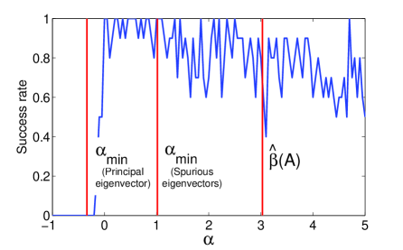
Fig. 1: Success rate for finding the best symmetric rank-one approximation of a symmetric tensor, as a function of shift parameter $\alpha$. The values for $\alpha_{min}$ come from Theorem 41 for the principal and spurious eigenvectors. Recall $\alpha>\alpha_{min}$ is sufficient but not necessary for stability. The best performance for SS-HOPM on rank-one approximation is when $\alpha$ is about the Theorem 41 threshold for the principal eigenvector but below the threshold for the spurious eigenvectors.

5 Conclusion

Our perturbative analysis establishes new facts about the structure of approximately-rank-one symmetric tensors, and the application of SS-HOPM to the rank-one approximation problem. We bound the closeness of the best symmetric rank-one approximation, and show that any sufficiently-large eigenpair informs us about the rank-one structure. We show that in high dimensions, most of the generalized Rayleigh quotient, whose critical points correspond to eigenvalues, is close to zero; as a consequence, the principal eigenvalue is prominent. We establish that for rank-one symmetric tensors, under mild conditions, SS-HOPM always moves an input vector towards the principal eigenvector. We also show that the principal eigenvector is a stable fixed point for SS-HOPM under a wide choice of shift parameters, and that SS-HOPM is guaranteed to converge to an eigenvector for a much smaller choice of $\alpha$ in the approximately-rank-one case (for an even number of modes) than the general case. A complete characterization of the basin of attraction for the principal eigenvector remains an open question. Finally, it is hoped that better understanding of the symmetric rank-one problem may lead to better of understanding of more complicated problems such as Independent Components Analysis.

6 Acknowledgements

Thanks to Mark Jacobson, Urmi Holz, Tammy Kolda, Dianne O’Leary, and Panayot Vassilevski for useful observations and guidance.

References

• [1] Lieven deΒ Lathauwer, Pierre Comon, Bart deΒ Moor, and Joos Vandewalle, Higher- order power methodβ€”application in independent component analysis, in Proceedings of the International Symposium on Nonlinear Theory Applications, 1995, pp.Β 91–96.
• [2] Christopher Hillar and Lek-Heng Lim, Most tensor problems are NP hard (http://arxiv.org/abs/0911.1393).
• [3] Eleftherios Kofidis and PhillipΒ A. Regalia, On the best rank-1 approximation of higher-order supersymmetric tensors, SIAM Journal on Matrix Analysis and Applications, 23 (2002), pp.Β 863–884.
• [4] TamaraΒ G. Kolda and JacksonΒ R. Mayo, Shifted power method for computing tensor eigenpairs, SIAM Journal on Matrix Analysis and Applications, 32 (2011), pp.Β 1095–1124.
• [5] Lek-Heng Lim, Singular values and eigenvalues of tensors: a variational approach, in Proceedings of the IEEE International Workshop on Computational Advances in Multi-Sensor Adaptive Processing, 2005, pp.Β 129–132.
• [6] V.Β Olshevsky, ed., Structured Matrices in Mathematics, Computer Science, and Engineering I, Contemporary Mathematics, American Mathematical Society, 2001, ch.Β Tensor approximation and signals processing applications.
• [7] Liqun Qi, Eigenvalues of a real supersymmetric tensor, Journal of Symbolic Computation, 40 (2005), pp.Β 1302–1324.
• [8] Liqun Qi, Fei Wang, and Yiju Wang, Z-eigenvalue methods for a global polynomial optimization problem, Mathematical Programming: Series A, 118 (2009), pp.Β 301–316.
• [9] G.Β W. Stewart and JiΒ guang Sun, Matrix Perturbation Theory, Academic Press, 1990.
• [10] Huahua Wang, Arindam Banerjee, and Daniel Boley, Modeling time varying covariance matrices in low dimensions, Tech. Report TR 10-017, Department of Computer Science and Engineering, University of Minnesota, 2010.
• [11] Yiju Wang and Liqun Qi, On the successive supersymmetric rank-1 decomposition of higher-order supersymmetric tensors, Numerical Linear Algebra with Applications, 14 (2007), pp.Β 503–519.
• [12] Tong Zhang and GeneΒ H. Golub, Rank-one approximation to high order tensors, SIAM Journal on Matrix Analysis and Applications, 23 (2001), pp.Β 534–550.