Boolean Satisfiability using Noise Based Logic

Abstract

In this paper, we present a novel algorithm to solve the Boolean Satisfiability (SAT) problem, using noise-based logic (NBL). Contrary to what the name may suggest, NBL is not a random/fuzzy logic system. In fact, it is a completely deterministic logic system. A key property of NBL is that it allows us to apply a superposition of many input vectors to a SAT instance at the same time, circumventing a key restriction and assumption in the traditional approach to solving SAT. By exploiting the superposition property of NBL, our NBL-based SAT algorithm can determine whether an instance is SAT or not in a single operation. A satisfying solution can be found by iteratively performing SAT check operations up to $n$ times, where $n$ is the number of variables in the SAT instance. Although this paper does not focus on the realization of an NBL-based SAT engine, such an engine can be conceived using analog circuits (wide-band amplifiers, adders and multipliers), FPGAs or ASICs. Additionally, we also discus scalability of our approach, which can apply to NBL in general. The NBL-based SAT engine described in this paper has been simulated in software for validation purposes.

I Introduction

Boolean Satisfiability (SAT) [1] is a core NP-complete problem which has been studied extensively. Given a set $V$ of variables ($n$ in all), and a collection $C$ of Conjunctive Normal Form (CNF) clauses over $V$ ($m$ in all), the SAT problem consists of determining if there is a satisfying truth assignment for $C$, and returning this truth assignment. The CNF expression $C$ is referred to as a SAT instance. If no satisfying assignment exists, $C$ is referred to as an unsatisfiable instance.

The applicability of SAT to several problem domains such as logic synthesis, formal verification, circuit testing, pattern recognition and others [2] has resulted in much effort devoted to devising efficient heuristics to solve SAT. Some of the more well-known complete approaches for SAT include [3, 4, 5, 6] and [7]. In addition, several incomplete or stochastic heuristics have been developed as well. A partial list of these are [8, 9, 10, 11, 12]. The complete approaches seek to find a satisfying solution (or to prove that none exists) by heuristically assigning a logic variable of the problem to ”1” or ”0”. By analyzing the consequences of such an assignment, a new variable is assigned, or a previously assigned variable is backtracked upon. This is continued until $C$ is satisfied, or the search space is exhausted (in which case $C$ is proven to be unsatisfiable)

Recently, it was shown that noise can be used to realize logic circuits [13, 14, 15]. We refer to this logic scheme as Noise-based Logic (NBL) in the sequel. In NBL, a plurality of pairwise uncorrelated noise sources (referred to as noise bits) are utilized. Each such noise source has zero mean, and all the sources have the same RMS value (assumed to be zero). It is important to point out that NBL is a deterministic logic scheme, and not fuzzy or probabilistic in nature. NBL can be utilized to realize multi-valued logic as well [15, 16].

The orthogonality property of the noise bits yields some powerful properties:

• Starting with $2n$ pairwise orthogonal basis noise sources, we can create a noise hyperspace of cardinality $2^{n}$, by appropriately multiplying these noise sources [15]. On a single wire, the additive superposition of any subset of this hyperspace can be transmitted, and this yields a total of $2^{2^{n}}$ possible logic values that can be transmitted on the wire. In effect the wire behaves like $2^{n}$ wires carrying binary valued signals.

• In addition, we can apply all possible inputs to an $n$ input NBL circuit simultaneously. Consider a combinational circuit with $n$ inputs $x_{1},x_{2},\cdots x_{n}$. For each input $x_{i}$, let us assume we have a noise source (noise bit) $N_{\overline{x_{i}}}$ to represent the $\overline{x_{i}}$ literal, and a noise source $N_{x_{i}}$ to represent the $x_{i}$ literal. Hence, for $1\leq i\leq n$, we may apply the input ($N_{x_{i}}+N_{\overline{x_{i}}}$) to the $i^{th}$ input of the circuit. This in effect means that we applied all $2^{n}$ inputs to the circuit simultaneously. We will see how this ends up being very important in Section III.

In this paper, we present an approach to solve the SAT problem utilizing NBL. The resulting approach can provide a SAT/UNSAT decision in a single operation, and can provide a satisfying input vector in a number of such operations which is linear in $n$. This is possible because NBL allows us to apply all $2^{n}$ inputs to the circuit simultaneously. Although no NBL circuits exist today, realizing the NBL-SAT solution approach of our paper would require widely studied, and ubiquitously available circuit components such as wideband amplifiers, analog adders and analog multipliers and low-pass filters. NBL-SAT may be implemented on FPGAs or ASICs as well. We hope that the result of this paper will encourage development of NBL circuits.

Before we list the contributions of this paper, we would like to reiterate that the NBL used in this paper is not probabilistic or fuzzy. Rather it is completely deterministic logic scheme. So the claims made in this paper are not probabilistic or fuzzy, but are completely deterministic.

The key contributions of this paper are:

• We show how NBL can solve the SAT problem. The resulting algorithm can determine if a problem is SAT or UNSAT in one operation, and can provide a satisfying assignment in $n$ operations, where $n$ is number of variables in the SAT problem.

• Although the focus of this paper is not to provide concrete realizations of the NBL based SAT algorithm, we show that such realizations are imminently realizable with existing technology

  • A hardware based NBL-SAT solver requires commonly available hardware components such as wide-band amplifiers, analog multipliers, analog adders, and low-pass filters, or even FPGAs or ASICs.

  • A software based NBL-SAT solver can be envisioned. Initial proof-of-correctness simulations of our algorithm were done on a MATLAB based realization of our algorithm.

  • Alternative realizations of NBL-SAT can be envisioned using sinusoidal signals [16] or Random Telegraph Waves [17].

The remainder of this paper is organized as follows. Section II discusses some previous work in this area. In Section III we describe our approach to solving the SAT problem using NBL. Section IV presents experimental results from a MATLAB based simulation which validates our approach. Section V discusses possible realizations of NBL-SAT, while conclusions are discussed in Section VI.

II Previous Work

The idea of noise based logic was recently developed, and initially described in [13]. In [14], the concept of NBL was extended to multi-valued signals as well, and it was shown that sinusoidal tones could be used instead of uncorrelated noise signals, as the information carriers. The idea of using an additive superposition of noise bits to generate a noise-based hyperspace idea was presented in [15]. Starting with $2n$ basis noise sources, it was shown how one could construct a hyperspace of $2^{n}$ noise sources using a linear number of additions and multiplications. By an additive superposition of any subset of this hyperspace, it was shown how a single wire could carry as many as $2^{2^{n}}$ symbols in it, effectively accomplishing the task of $2^{n}$ binary-valued wires.

Several derivative papers [18, 19, 17] of these works developed the idea of noise based logic further, using pulse based [18, 19] or Random Telegraph Wave (RTW) [17] based signals. A VLSI implementation of NBL (using sinusoidal signals as information carriers) was presented in [16]. In this paper, the specialized and restricted version of NBL used sinusoids. In particular the logic 1 and logic 0 signals were chosen to be anti-correlated, in order to mimic binary logic and demonstrate the viability of the approach. It was shown that with existing MOSFETs, one can realize gates using sinusoidal logic. To the best of the authors’ knowledge, there has been no effort to date, to realize true NBL gates or circuits.

Just like NBL, quantum computers have the capability of applying a superposition of input values to a quantum circuit. In the past, there has been work in the realm of quantum computing [20, 21, 22] focusing on solving SAT on quantum computers. There are some precise differences between these papers and the NBL based SAT engine described in this paper:

• In contrast to our approach, [20, 21, 22] only solve the problem of determining whether a SAT instance is satisfiable or unsatisfiable. Our approach, over and above that of [20, 21, 22], provides an algorithm to determine the satisfying assignment (if one exists) using a linear number of NBL-SAT checks.

• Also, our NBL based SAT algorithm is realizable using existing ubiquitous circuit components (such as wide-band amplifiers, analog adders, analog multipliers and filters). In contrast, the field of quantum computing is extremely young, without the ability to realize even medium sized quantum circuits, severely hampering the applicability of the quantum SAT algorithm of [20, 21, 22].

III Our Approach

Before discussing our NBL-SAT algorithm, we first provide definitions related to topics of Boolean Satisfiability, NP-completeness, and Noise-based Logic.

III-A Definitions

Definition 1

A literal or a literal function is a binary variable $x$ or its negation $\overline{x}$.

Definition 2

A cube is a conjunction (AND) of one or more literal functions, i.e. $x_{1}x_{2}\overline{x_{3}}$.

Definition 3

A clause is a disjunction (OR) of one or more literal functions, i.e. $(x_{1}+x_{2})$.

Definition 4

A Conjunctive Normal Form (CNF) formula consists of a conjunction of $m$ clauses $c_{1},c_{2}\ldots c_{m}$. Each clause $c_{i}$ consists of the disjunction of $k_{i}$ literals.

Definition 5

A CNF formula is said to be satisfied if each of the $m$ clauses of the CNF formula simultaneously evaluate to true.

A CNF formula is also referred to as a logical product of sums. Thus, to satisfy the CNF formula, at least one literal in each clause must evaluate to true.

Definition 6

Boolean Satisfiability (SAT): Given a Boolean formula $S$ on a set of binary variables $X=\{x_{1},x_{2},x_{3}\cdots x_{n}\}$, expressed in Conjunctive Normal Form (CNF), the objective of SAT is to identify an assignment of the binary variables in $X$ that satisfies $S$. If no such assignment exists, this should be indicated.

For example, consider the formula $S(x_{1},x_{2},x_{3})=(x_{1}+\overline{x_{2}})\cdot(x_{1}+x_{2}+x_{3})$. This formula consists of 3 variables, 2 clauses, and 4 literals. This particular formula is satisfiable, and a satisfying assignment is $<x_{1},x_{2},x_{3}>\,=\,<0,0,1>$, which can be expressed as the satisfying cube $\overline{x_{1}}\,\overline{x_{2}}\,x_{3}$. The CNF expression $S$ is often referred to as a SAT instance in the literature.

SAT is one of the most well known NP-complete problems. As such, therefore, there are no known polynomial time algorithms to solve SAT. Note that the definition of NP-completeness is premised on the assumption that a Universal Turing Machine (UTM) is used to perform operations to solve the decision problem $C$. In this paper, we sidestep this particular assumption. In particular, using NBL to solve SAT, we are able to apply a superposition of all inputs (candidate solutions) to the problem instance. This superposition property allows us to verify all solutions simultaneously to determine if the problem is satisfiable (or not) in a single operation, and if satisfiable, to provide a satisfying solution in a number of operations that is linear in $n$.

The remainder of this sub-section presents some definitions pertaining to Noise-based Logic (NBL).

Definition 7

Independent Noise Processes: Consider two noise processes $V_{i}(t)$ and $V_{j}(t)$. These noise processes are independent iff the correlation operator $\langle\rangle$ applied to $V_{i}(t)$ and $V_{j}(t)$ yields

$\langle V_{i}(t)V_{j}(t)\rangle=\delta_{i,j}$

where $\delta_{i,j}$ is the Kronecker symbol ($\delta_{i,j}=1$ when $i=j$, and $\delta_{i,j}=0$ otherwise.

Definition 8

Basis (Reference) Noise Processes (Bits): Consider $M$ noise processes $V_{1}(t),V_{2}(t),\cdots,V_{M}(t)$. If these processes are pairwise independent, then $V_{1}(t),V_{2}(t),\cdots,V_{M}(t)$ are referred to as basis (reference) noise processes (bits).

For convenience, we assume that all the noise processes in the sequel have a zero mean, and a zero RMS value.

Consider two orthogonal basis noise bits $V_{i}(t)$ and $V_{j}(t)$ ($i\neq j$). The product $Z_{i,j}(t)=V_{i}(t)\cdot V_{j}(t)$ of two orthogonal basis noise bits is orthogonal to $V_{k}(t)$ ($k=1,2,\cdots,M$). This property was used [15] to realize a logic hyperspace. In other words,

$\langle Z_{i,j}(t),V_{k}(t)\rangle$ = 0

Definition 9

Noise-based Logic Hyperspace: Using $2M$ basis noise bits $V^{0}_{1}(t),V^{1}_{1}(t),\cdots V^{0}_{m}(t),V^{1}_{m}(t)$, we can compute a noise hyperspace $\cal{H}$ with dimensionality $2^{M}$, by multiplying these noise bits appropriately, and performing their additive superposition as follows:

$$\cal{H} = V^{0}_{1}(t)\cdot V^{0}_{2}(t)\cdots V^{0}_{m-1}(t)+$$

$$V^{0}_{1}(t)\cdot V^{0}_{2}(t)\cdots V^{1}_{m-1}(t)+$$

$$\cdots+V^{1}_{1}(t)\cdot V^{1}_{2}(t)\cdots V^{1}_{m-1}(t)$$

Example 1: Consider four orthogonal basis noise bits $V^{0}_{1}(t),V^{1}_{1}(t),V^{0}_{2}(t),V^{1}_{2}(t)$. The noise-based logic hyperspace consists of four hyperspace elements $V^{0}_{1}(t)\cdot V^{0}_{2}(t)$, $V^{0}_{1}(t)\cdot V^{1}_{2}(t)$, $V^{1}_{1}(t)\cdot V^{0}_{2}(t)$, $V^{1}_{1}(t)\cdot V^{1}_{2}(t)$.

The power of the noise-based hyperspace is evidenced by the fact that starting from $2M$ basis noise sources, we can construct a hyperspace of size $2^{M}$. Now an additive superposition of any subset of elements from this hyperspace can be transmitted along a wire.

In the remainder of this paper, we will refer to noise sources as $N$ instead of $N(t)$.

III-B Generating all $2^{n}$ Minterms in an NBL Additive Superposition

Before we describe our NBL based SAT algorithm, we first discuss a means of constructing the additive superposition of all input vectors for a problem [15].

Consider a problem on $n$ binary valued variables $x_{1},x_{2},\cdots,x_{n}$. For each variable $x_{i}$, we define two basis noise sources $N_{x_{i}}$ and $N_{\overline{x_{i}}}$, for the negative and positive literals of $x_{i}$ respectively. This requires a total of $2n$ basis noise sources. Now, we can construct the product

$$T=(N_{x_{1}}+N_{\overline{x_{1}}})\cdot(N_{x_{2}}+N_{\overline{x_{2}}})\cdots(N_{x_{n}}+N_{\overline{x_{n}}})$$ (1)

If $T$ were expanded out, it is easy to see that $T$ is the additive superposition of $2^{n}$ products of basis noise sources. Each product corresponds to a noise-based minterm on the $n$ variable space.

Example 3: Suppose $n=3$. Then, if $T$ were expanded out, we get

$T=(N_{x_{1}}\cdot N_{x_{2}}\cdot N_{x_{3}})+(N_{x_{1}}\cdot N_{x_{2}}\cdot N_{\overline{x_{3}}})+(N_{x_{1}}\cdot N_{\overline{x_{2}}}\cdot N_{x_{3}})+(N_{x_{1}}\cdot N_{\overline{x_{2}}}\cdot N_{\overline{x_{3}}})+(N_{\overline{x_{1}}}\cdot N_{x_{2}}\cdot N_{x_{3}})+(N_{\overline{x_{1}}}\cdot N_{x_{2}}\cdot N_{\overline{x_{3}}})+(N_{\overline{x_{1}}}\cdot N_{\overline{x_{2}}}\cdot N_{x_{3}})+(N_{\overline{x_{1}}}\cdot N_{\overline{x_{2}}}\cdot N_{\overline{x_{3}}})$

In other words, using Equation 1, we are able to generate the additive superposition of all $2^{n}$ minterms of the binary space. This is generated with a linear number of noise sources, and a linear number of analog adders and multipliers.

An important variation of the above idea is that we can bind a subset of variables to any literal value in $T$ above, and generate an additive superposition of the minterms that are in the cube subspace of the bound variables. In other words, suppose we bind variables $X=\{x_{i},x_{i+1},\cdots,x_{i+p-1}\}$ to literals $l_{i},l_{i+1},\cdots,l_{i+p-1}$ respectively, where $p<n$, then we generate the additive superposition of all minterms in the cube subspace $l_{i}\cdot l_{i+1}\cdot l_{i+2}\cdots l_{i+p-1}$.

Example 4: In Example 3, if we bind variable $x_{1}$ to literal $\overline{x_{1}}$, then $T_{\overline{x_{1}}}=(N_{\overline{x_{1}}}+0)\cdot(N_{x_{2}}+N_{\overline{x_{2}}})\cdots(N_{x_{n}}+N_{\overline{x_{n}}})$. If $T_{\overline{x_{1}}}$ were expanded out, we would get

$T_{\overline{x_{1}}}=(N_{\overline{x_{1}}}\cdot N_{x_{2}}\cdot N_{x_{3}})+(N_{\overline{x_{1}}}\cdot N_{x_{2}}\cdot N_{\overline{x_{3}}})+(N_{\overline{x_{1}}}\cdot N_{\overline{x_{2}}}\cdot N_{x_{3}})+(N_{\overline{x_{1}}}\cdot N_{\overline{x_{2}}}\cdot N_{\overline{x_{3}}})$

Thus $T_{\overline{x_{1}}}$ is the additive superposition of all the minterms in the cube subspace $\overline{x_{1}}$.

Using the construction of $T$ and $T_{v}$ subspace above, we now discuss our NBL-SAT algorithm.

III-C SAT to NBL-SAT Transformation

In this subsection, we described the process of transforming a SAT decision problem $S$ into an equivalent NBL formula $S_{N}$. Consider a decision problem expressed as a CNF $S$ with $m$ clauses ($S=c_{1}\cdot c_{2}\cdots c_{m}$) on a set of binary variables $X=(x_{1},x_{2},\cdots,x_{n})$. We would like to determine if $S$ is satisfiable, and if so, find a satisfying assignment. $S_{N}$ is comprised of the product of 2 sets of clauses $\tau_{N}$ and $\Sigma_{N}$, where $\tau_{N}$ contains all $2^{n}$ valid minterms for the instance $S$, while $\Sigma_{N}$ contains all satisfying minterms for $S$. These clauses are discussed in detail in the following.

For each clause $c_{j}$, we create $2n$ independent basis noise sources which are used to represent the positive and negative literal of each variable $x_{1},x_{2},\cdots,x_{M}$. Let $N^{j}_{x_{i}}$ be the noise source corresponding to literal $x_{i}$ in clause $c_{j}$, and $N^{j}_{\overline{x_{i}}}$ be the noise source corresponding to literal $\overline{x_{i}}$ in clause $c_{j}$. In total, we create $2mn$ independent basis noise sources as there are $m$ clauses, each requiring $2n$ noise sources. Note that the noise sources are independent across clauses, such that the product of any noise (for any variable $x_{p}$ and $x_{q}$) from clauses $c_{j}$ and $c_{k}$ where $j\neq k$ has a zero mean ($N^{j}_{x_{p}}\cdot N^{k}_{x_{q}}=0$).

Construction of $\tau_{N}$: First we construct the noise hyperspace $\tau_{N}$ which contains all $2^{n}$ valid minterms to be applied to the SAT instance $\Sigma_{N}$. The hyperspace $\tau_{N}$ is constructed following Equation 1, except the two basis noise sources $N_{x_{i}}$ and $N_{\overline{x_{i}}}$ for literals $x_{i}$ and $\overline{x_{i}}$ are replaced with the products $N^{1}_{x_{i}}N^{2}_{x_{i}}\cdots N^{m}_{x_{i}}$ and $N^{1}_{\overline{x_{i}}}N^{2}_{\overline{x_{i}}}\cdots N^{m}_{\overline{x_{i}}}$ respectively. These products correspond to the product of noise sources for literals $x_{i}$ and $\overline{x_{i}}$ respectively, used in all clauses for $\Sigma_{N}$.

$$\tau_{N} = ((N^{1}_{x_{1}}N^{2}_{x_{1}}\cdots N^{m}_{x_{1}})+(N^{1}_{\overline{x_{1}}}N^{2}_{\overline{x_{1}}}\cdots N^{m}_{\overline{x_{1}}}))$$ (2)

$$\cdot((N^{1}_{x_{2}}N^{2}_{x_{2}}\cdots N^{m}_{x_{2}})+(N^{1}_{\overline{x_{2}}}N^{2}_{\overline{x_{2}}}\cdots N^{m}_{\overline{x_{2}}}))$$

$$\cdots((N^{1}_{x_{n}}N^{2}_{x_{n}}\cdots N^{m}_{x_{n}})+(N^{1}_{\overline{x_{n}}}N^{2}_{\overline{x_{n}}}\cdots N^{m}_{\overline{x_{n}}}))$$

Construction of $\Sigma_{N}$: Now we construct the NBL-based SAT instance $\Sigma_{N}$ from the SAT instance $S$ by replacing the positive literal of variable $v$ in clause $c_{j}$ by cube subspace $T^{j}_{v}$, and the negative literal of variable $v$ in clause $c_{j}$ by noise source $T^{j}_{\overline{v}}$. By binding the the variable $v$ to the literal value, the cube subspace $T^{j}_{v}$ or $T^{j}_{\overline{v}}$ is an additive superposition of minterms containing the literal value which satisfies clause $c_{j}$.

Example 5: Consider the CNF formula $S=c_{1}\cdot c_{2}\cdot c_{3}\cdot c_{4}=(\overline{x_{1}})\cdot(x_{2}+x_{3})\cdot(x_{1}+\overline{x_{3}})\cdot(\overline{x_{1}}+\overline{x_{2}}+x_{3})$. The NBL-SAT instance $\Sigma_{N}$ is as follows:

$\Sigma_{N}=(T^{1}_{\overline{x_{1}}})\cdot(T^{2}_{x_{2}}+T^{2}_{x_{3}})\cdot(T^{3}_{x_{1}}+T^{3}_{\overline{x_{3}}})\cdot(T^{4}_{\overline{x_{1}}}+T^{4}_{\overline{x_{2}}}+T^{4}_{x_{3}})$

When $\Sigma_{N}$ is expanded out, the noise vectors for minterms from each clause form products with noise vectors of minterms from all other clauses. A valid satisfying minterm for $\Sigma_{N}$ would be such that its final noise product contains a product of noise vectors from all clauses that represent the same minterm. All other combination of noise vectors are logically invalid.

Consider a SAT formula $S$ where number of variables and clauses are $n=2$ and $m=2$ respectively. An example of a valid noise-based minterm is:

$N^{1}_{x_{1}}N^{2}_{x_{1}}N^{1}_{\overline{x_{2}}}N^{2}_{\overline{x_{2}}}$

which corresponds to the minterm $x_{1}\,\overline{x_{2}}$ of $S$. An example of an invalid noise-based minterm is:

$N^{1}_{x_{1}}N^{2}_{\overline{x_{1}}}N^{1}_{x_{2}}N^{2}_{x_{2}}$

Which corresponds to the term $x_{1}\,\overline{x_{1}}\,x_{2}$ of $S$.

Thus $\Sigma_{N}$ is the additive superposition of all valid (satisfying) and invalid minterms of the SAT instance. Since $\tau_{N}$ only contains all valid minterms as shown in Equation 2, the product of $\tau_{N}\cdot\Sigma_{N}$ is the additive superposition of the self-correlation of each of the valid minterms. The average value of $\tau_{N}\cdot\Sigma_{N}$ is zero if the instance $S$ is unsatisfiable, and positive if the instance $S$ is satisfiable.

III-D Satisfiability Check using NBL-SAT

Algorithm 1 describes the procedure for a single operation satisfiability checking using NBL-SAT. After formulation of NBL-SAT $\Sigma_{N}$ and hyperspace $\tau_{N}$, the check for satisfiability is done with an observation of $S_{N}=\tau_{N}\cdot\Sigma_{N}$. If $S_{N}$ has a zero average, then we conclude $S$ is unsatisfiable. If on the other hand, $S_{N}$ has a positive average value, then $S$ is satisfiable.

1:  $NBL-SAT\_check(S_{N})$

2:  $S_{N}\leftarrow(\tau_{N}\cdot\Sigma_{N})$

3:  if $S_{N}$ output has a zero average then

4:     return($S$ is unsatisfiable)

5:  else

6:     return($S$ is satisfiable)

7:  end if

Algorithm 1 Pseudocode of NBL-SAT checker

The key to the single operation SAT check achieved by this algorithm are the superposition and correlation properties of the noise basis sources. In $\Sigma_{N}$, each clause $c_{j}$ contains any number of cube subspaces $T^{j}_{v}$. The disjunction of all the $T^{j}_{v}$ in clause $c_{j}$ result in a new noise vector $Z^{j}$. Thus $Z^{j}$ is the additive superposition of all noise-based minterms that satisfy clause $c_{j}$. Hence $\Sigma_{N}$ includes the additive superposition of all noise-based minterms that satisfy $S$. Multiplying $\Sigma_{N}$ with $\tau_{N}$ simply yields the additive superposition of the self correlation of the noise-based minterms of $S$.

The output of $\Sigma_{N}$ is the conjunction (product) of all $Z^{j}$ noise vectors from the clauses. We recall that the product of two independent noise sources is 0. As $\tau_{N}$ is the additive superposition of valid minterms for $S$, then the product $\tau_{N}\cdot\Sigma_{N}=0$ only in the case where $\Sigma_{N}$ and $\tau_{N}$ do not share any noise vectors, and hence, no minterm exists in $\Sigma_{N}$ that correlates to any of the valid minterms in $\tau_{N}$. If $S_{N}=0$ or has a zero average, then there is no valid minterm that exists across all clauses and we conclude $S$ is unsatisfiable (line 4).

However, if $\Sigma_{N}$ and $\tau_{N}$ contain common minterm(s), the product of the noise vectors results in a positive average for $S_{N}$. Then if $\tau_{N}\cdot\Sigma_{N}$ has a positive DC offset, we can conclude a common satisfying minterm exists across all clauses (line 6).

A demonstration of the algorithm is shown in Examples 6 and 7.

Example 6: Consider the CNF formula $S=(x_{1}+\overline{x_{2}})\cdot(\overline{x_{1}}+\overline{x_{2}})$. The NBL-SAT instance is as follows:

$\Sigma_{N}=(T^{1}_{x_{1}}+T^{1}_{\overline{x_{2}}})\cdot(T^{2}_{\overline{x_{1}}}+T^{2}_{\overline{x_{2}}})$

By expanding $T^{j}_{x_{i}}$ to show the minterms:

$\Sigma_{N}=(N^{1}_{x_{1}}N^{1}_{x_{2}}+N^{1}_{x_{1}}N^{1}_{\overline{x_{2}}}+N^{1}_{\overline{x_{1}}}N^{1}_{\overline{x_{2}}})\cdot(N^{2}_{x_{1}}N^{2}_{\overline{x_{2}}}+N^{2}_{\overline{x_{1}}}N^{2}_{x_{2}}+N^{2}_{\overline{x_{1}}}N^{2}_{\overline{x_{2}}})$

The minterms $x_{1}\overline{x_{2}},\overline{x_{1}}\,\overline{x_{2}}$ exist in all clauses, which will have the noise products $N^{1}_{x_{1}}N^{2}_{x_{1}}N^{1}_{\overline{x_{2}}}N^{2}_{\overline{x_{2}}}$, $N^{1}_{\overline{x_{1}}}N^{2}_{\overline{x_{1}}}N^{1}_{\overline{x_{2}}}N^{2}_{\overline{x_{2}}}$ respectively in $\Sigma_{N}$.

The valid minterm hyperspace $\tau_{N}$ is as follows:

$\tau_{N}=(N^{1}_{x_{1}}N^{2}_{x_{1}}+N^{1}_{\overline{x_{1}}}N^{2}_{\overline{x_{1}}})\cdot(N^{1}_{x_{2}}N^{2}_{x_{2}}+N^{1}_{\overline{x_{2}}}N^{2}_{\overline{x_{2}}})$

$\tau_{N}=N^{1}_{x_{1}}N^{2}_{x_{1}}N^{1}_{x_{2}}N^{2}_{x_{2}}+N^{1}_{x_{1}}N^{2}_{x_{1}}N^{1}_{\overline{x_{2}}}N^{2}_{\overline{x_{2}}}+N^{1}_{\overline{x_{1}}}N^{2}_{\overline{x_{1}}}N^{1}_{x_{2}}N^{2}_{x_{2}}+N^{1}_{\overline{x_{1}}}N^{2}_{\overline{x_{1}}}N^{1}_{\overline{x_{2}}}N^{2}_{\overline{x_{2}}}$

The noise products for the minterms $x_{1}\,\overline{x_{2}}$, $\overline{x_{1}}\,\overline{x_{2}}$ exist in both $\Sigma_{N}$ and $\tau_{N}$. The result $S_{N}=\tau_{N}\cdot\Sigma_{N}$ will be the additive superposition of the self-correlation of these two noise products and $S_{N}$ will thus have a positive average, concluding this example as satisfiable.

Example 7: Consider the CNF formula $S=(x_{1})\cdot(\overline{x_{1}})$. The NBL-SAT instance is as follows:

$\Sigma_{N}=(T^{1}_{x_{1}})\cdot(T^{2}_{\overline{x_{1}}})$

By expanding $T^{j}_{x_{i}}$ to show the minterms and noise products:

$\Sigma_{N}=N^{1}_{x_{1}}N^{2}_{\overline{x_{1}}}$

The valid minterm hyperspace is as follows:

$\tau_{N}=N^{1}_{x_{1}}N^{2}_{x_{1}}+N^{1}_{\overline{x_{1}}}N^{2}_{\overline{x_{1}}}$

The noise vectors in $\Sigma_{N}$ and $\tau_{N}$ are orthogonal as they do not contain any common minterms. The result $S_{N}=\tau_{N}\cdot\Sigma_{N}$ will have a zero average, concluding that this example is unsatisfiable.

Theorem III.1

If the product of the NBL-SAT instance $\Sigma_{N}$ and hyperspace $\tau_{N}$ produces a zero average, then $S=f(x_{1},x_{2},\cdots,x_{M})$ is unsatisfiable.

Proof:

If a subset of clauses $\{c_{j},c_{j+1},\cdots,c_{k}\}$ in $S$ are unsatisfiable, then there are no common minterms among $c_{j},c_{j+1},\cdots,c_{k}$. As such, the corresponding noise vectors $Z^{j},Z^{j+1},\cdots,Z^{k}$, which contain the additive superposition of minterms that satisfy $c_{j},c_{j+1},\cdots,c_{k}$ respectively, will form a superposition of logically invalid noise minterms (i.e. $N^{j}_{x_{i}}N^{k}_{\overline{x_{i}}}$). As $\tau_{N}$ contains only valid minterms by construction, $\Sigma_{N}$ and $\tau_{N}$ will be uncorrelated, and the product $\tau_{N}\cdot\Sigma_{N}$ will produce a zero average output. ∎

Note that two key observations can be made at this stage:

• Applying the test of Theorem III.1 allows us to determine if $S$ is SAT with a single operation.

• The reason why we are able to perform the SAT check with a single operation is that we are able to effectively and simultaneously apply all minterms to the NBL-SAT instance, since each of the minterms in NBL are orthogonal basis noise vectors. This is not possible in traditional SAT solvers.

III-E Algorithm to Determine Satisfying Assignment using NBL-SAT

Algorithm 2 describes the NBL-SAT procedure to determine the satisfying assignment for a SAT instance $S$. It is assumed that Algorithm 1 has been run and has shown $S$ to be satisfiable before Algorithm 2 is invoked.

1:  $NBL-SAT\_satisfying\_assignment\_determination(S_{N})$

2:  $Result=\phi$

3:  for $i$ = 1 to $n$ do

4:     $\tau_{N}^{red}\leftarrow(\tau_{N}$ with variable $x_{i}$ bound to 1)

5:     $S_{N}^{red}\leftarrow(\tau_{N}^{red}\cdot\Sigma_{N}$)

6:     if NBL-SAT_check($S_{N}^{red}$) is unsatisfiable then

7:        $Result\leftarrow Result\cup\overline{x_{i}}$

8:        $\tau_{N}^{red}\leftarrow(\tau_{N}$ with variable $x_{i}$ bound to 0)

9:     else

10:        $Result\leftarrow Result\cup x_{i}$

11:     end if

12:     $\tau_{N}\leftarrow\tau_{N}^{red}$

13:  end for

14:  return $Result$

Algorithm 2 Pseudocode of NBL-SAT satisfying assignment determination

Algorithm 2 starts by initializing the result to $\phi$ (line 2). We iterate over all $n$ variables of the problem (line 3). In the $i^{th}$ iteration, we take the current reduced hyperspace $\tau_{N}$, and bind the variable $x_{i}$ to 1 (line 4). By binding the variable $x_{i}$ to 1, we limit the reduced hyperspace $\tau_{N}^{red}$ to contain only valid minterms in the $x_{i}$ subspace. In essence, we are testing to see whether the current $S_{N}^{red}$ has a satisfying solution in the $x_{i}$ subspace. If the NBL-SAT_check of $S_{N}^{red}$ returns ”unsatisfiable”, then the solution is in the $\overline{x_{i}}$ subspace (since $S_{N}$ is known to be satisfiable a-priori, given that that Algorithm 1 has already been run). Hence we append $\overline{x_{i}}$ to the result (line 7), and continue further processing after binding variable $x_{i}$ to 0 (line 8). If $\Sigma_{N}^{red}$ is satisfiable, then the solution is in the $x_{i}$ subspace, and we append $x_{i}$ to the result (line 10). Before continuing the next iteration, we update $\tau_{N}$ with $\tau_{N}^{red}$ (line 12), to ensure that future iterations inherit the variable binding that was conducted in the current iteration. The result is finally returned in line 14.

Example 8: Consider the SAT instance of Example 6, $S=(x_{1}+\overline{x_{2}})\cdot(\overline{x_{1}}+\overline{x_{2}})$, which has been known to be satisfiable according to Algorithm 1. The NBL-SAT formula is as follows:

$\Sigma_{N}=(N^{1}_{x_{1}}N^{1}_{x_{2}}+N^{1}_{x_{1}}N^{1}_{\overline{x_{2}}}+N^{1}_{\overline{x_{1}}}N^{1}_{\overline{x_{2}}})\cdot(N^{2}_{x_{1}}N^{2}_{\overline{x_{2}}}+N^{2}_{\overline{x_{1}}}N^{2}_{x_{2}}+N^{2}_{\overline{x_{1}}}N^{2}_{\overline{x_{2}}})$

$\tau_{N}=(N^{1}_{x_{1}}N^{2}_{x_{1}}+N^{1}_{\overline{x_{1}}}N^{2}_{\overline{x_{1}}})\cdot(N^{1}_{x_{2}}N^{2}_{x_{2}}+N^{1}_{\overline{x_{2}}}N^{2}_{\overline{x_{2}}})$

$S_{N}=\Sigma_{N}\cdot\tau_{N}$

$\Sigma_{N}$ contains two valid noise minterms $N^{1}_{x_{1}}N^{2}_{x_{1}}N^{1}_{\overline{x_{2}}}N^{2}_{\overline{x_{2}}}$, $N^{1}_{\overline{x_{1}}}N^{2}_{\overline{x_{1}}}N^{1}_{\overline{x_{2}}}N^{2}_{\overline{x_{2}}}$ which are $x_{1}\,\overline{x_{2}},\overline{x_{1}}\,\overline{x_{2}}$ respectively.

Now in the first iteration of Algorithm 2, we bind variable $x_{1}$ to 1 (line 4), yielding

$\tau_{N}^{red}=(N^{1}_{x_{1}}N^{2}_{x_{1}}+0)\cdot(N^{1}_{x_{2}}N^{2}_{x_{2}}+N^{1}_{\overline{x_{2}}}N^{2}_{\overline{x_{2}}})$

$\tau_{N}^{red}=N^{1}_{x_{1}}N^{2}_{x_{1}}N^{1}_{x_{2}}N^{2}_{x_{2}}+N^{1}_{x_{1}}N^{2}_{x_{1}}N^{1}_{\overline{x_{2}}}N^{2}_{\overline{x_{2}}}$

$S_{N}^{red}=\Sigma_{N}\cdot\tau_{N}^{red}$

Thus $S_{N}^{red}$ has a positive average value as the noise minterm $N^{1}_{x_{1}}N^{2}_{x_{1}}N^{1}_{\overline{x_{2}}}N^{2}_{\overline{x_{2}}}$ exists in both $\Sigma_{N}$ and $\tau_{N}^{red}$. The NBL-SAT_check will return that $S_{N}^{red}$ is satisfiable, and $x_{1}$ is appended to the (initially empty) result (line 7) and we update $\tau_{N}\leftarrow\tau_{N}^{red}$.

In the second iteration, we bind variable $x_{2}$ to 1, yielding

$\tau_{N}^{red}=(N^{1}_{x_{1}}N^{2}_{x_{1}}+0)\cdot(N^{1}_{x_{2}}N^{2}_{x_{2}}+0)$

$\tau_{N}^{red}=N^{1}_{x_{1}}N^{2}_{x_{1}}N^{1}_{x_{2}}N^{2}_{x_{2}}$

$S_{N}^{red}=\Sigma_{N}\cdot\tau_{N}^{red}$

The $S_{N}^{red}$ has a zero average value and the NBL-SAT_check will return that $S_{N}^{red}$ is unsatisfiable, hence $\overline{x_{2}}$ is appended to the final result $x_{1}\,\overline{x_{2}}$ (line 10) which is our satisfying assignment for the example.

Note that Algorithm 2 yields a satisfying minterm. It can be easily modified to return satisfying cubes. To do this, each iteration would bind a variable $x_{i}$ to both 1 and 0. If the resulting $S_{N}^{red}$ outputs both have a positive average value, then variable $x_{i}$ would be omitted from the result.

III-F Scaling Issues

In order to discuss how NBL-SAT scales with the number of variables and clauses, consider 3-SAT instances (in which each clause has 3 literals) with $n$ variables and $m$ clauses. We assume that each basis noise source ($N^{j}_{x_{i}}$) is a uniform random variable between [-0.5, 0.5]. Recall that the average value of $\tau_{N}\cdot\Sigma_{N}$ is proportional to the number of satisfying minterms, since such minterms are present in both $\tau_{N}$ and $\Sigma_{N}$. Hence the ability of NBL-SAT to discriminate between an instance with one satisfying minterm and another instance which is unsatisfiable needs to be considered. We define the SNR of NBL-SAT as

SNR = $\frac{\hat{\mu_{1}}-3\hat{\sigma_{1}}}{\hat{\mu_{0}}+3\hat{\sigma_{0}}}$

where $\hat{\mu_{i}}$ is the expectation of the mean of the average value of $\tau_{N}\cdot\Sigma_{N}$ when there are $i$ satisfying minterms, and $\hat{\sigma_{i}}$ is the expectation of the standard deviation of the average value of $\tau_{N}\cdot\Sigma_{N}$, when there are $i$ satisfying minterms. Note that $\hat{\mu_{0}}$ = 0. Assuming that there are $N$ samples in each noise source, we have:

$\hat{\mu_{1}}=E(\frac{1}{N}\Sigma_{i=1}^{N}\{\Pi_{j=1}^{nm}x_{j}^{2}\})$

where $x_{j}$ is uniformly distributed within [-0.5, 0.5]. The product is over $nm$ since there are $nm$ noise products in any satisfying minterm in NBL-SAT. Simplifying, we have $\hat{\mu_{1}}=(\frac{1}{12})^{nm}$.

Similarly, the unbiased estimate of the variance of the mean of the product of $nm$ independent uniform distributions [23] (over $N$ samples) is given by $\hat{\sigma^{2}}=\frac{1}{N-1}(\frac{1}{12})^{2nm}$.

Now the total number of products in a NBL-based 3-SAT instance with $n$ variables and $m$ clauses is $(2^{n})\cdot(2^{n}-2^{n-3})^{m}$ $\sim$ $O(2^{nm})$. The first term refers to the number of products of $\tau_{N}$, while the second term is the number of products in $\Sigma_{N}$. Since these $O(2^{nm})$ products are independent, their variances will add up, and so we have $\hat{\sigma_{1}}=\hat{\sigma_{0}}=\frac{1}{\sqrt{N-1}}(\frac{1}{12})^{nm}\cdot 2^{nm}$.

For SNR $\gg$ 1, we can ignore $\hat{\sigma_{1}}$ in the SNR expression, yielding

SNR = $\frac{\hat{\mu_{1}}}{3\hat{\sigma_{0}}}=\frac{\sqrt{N-1}}{3\cdot 2^{nm}}$.

Note that if it is known that the instance has $K$ satisfying minterms, then the SNR expression above is multiplied by $K$.

IV Experimental Results

To validate our NBL-SAT algorithm, we simulated several small NBL-SAT $S_{N}$ instances and corresponding $T_{N}$ hyperspaces in MATLAB. In our simulations, each basis noise source ($N^{j}_{x_{i}}$) is a uniform random variable between [-0.5, 0.5]. Each instance is simulated until the mean value of $S_{N}$ has converged to the third significant digit or until $10^{8}$ noise samples have been reached. Our experiments focus on the SAT checker from Algorithm 1, as the satisfying assignment determination from Algorithm 2 simply consists of iterative applications of the SAT checker.

We use the following two examples, one unsatisfiable and one satisfiable, to validate the correctness of our scheme.

$S_{UNSAT}=(x_{1}+x_{2})\cdot(x_{1}+\overline{x_{2}})\cdot(\overline{x_{1}}+x_{2})\cdot(\overline{x_{1}}+\overline{x_{2}})$

$S_{SAT}=(x_{1}+\overline{x_{2}})\cdot(\overline{x_{1}}+\overline{x_{2}})\cdot(x_{1}+\overline{x_{2}})\cdot(\overline{x_{1}}+\overline{x_{2}})$

The first clause in our satisfiable example is redundant, but brings the number of clauses $m$ to 4 and make the $S_{N}$ values comparable with our unsatisfiable example which also has $m=4$. In Figure 1, the average mean values of $S_{N}$ of both examples are plotted as a function of number of noise samples.

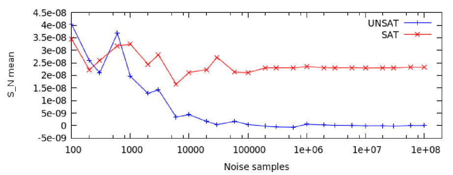
Figure 1: $S_{N}$ mean for UNSAT and SAT instances

V Realizing an NBL-based SAT Engine

The NBL-based SAT algorithm is easily realized using existing hardware and software based approaches. We devote this section to a discussion on possible realizations.

A first observation we make in this regard is that instead of using uncorrelated noise sources as the basis vectors, we could utilize sinusoidal signals as the basis vectors [14, 16]. Assuming that the highest frequency sinusoid realizable in today’s technology has a frequency $F$, (typically in the 10s of GHz), and that all the basis sinusoids are equi-spaced with a frequency difference of $f$ between adjacent sinusoids, we could realize $F/f$ variables for the Sinusoid-based Logic (SBL) SAT engine. Minimizing $f$ would be a key design criterion, allowing us to implement a large number of variables. A small value of $f$ would require the low-pass filters of high order, yielding a more complex circuit. The tradeoff of circuit complexity versus number of variables remains an open exercise.

Using the above ideas, a hardware based NBL-based SAT field-programmable engine can be envisioned as well. Such an engine would have a plurality of adders (implementing configurable clauses), multipliers (implementing the conjunction operation among the clauses), and noise sources (which could potentially be made up of wideband amplifiers which amplify a resistor’s thermal noise, or realized using pseudorandom number generator). In an SBL based engine, on-chip sinusoidal oscillators of different frequencies [24, 25, 26] could be utilized. Such an engine would have an on-chip correlator block as well. Having such a reconfigurable engine would allow the user to load their specific SAT instance on this engine, and run it using the algorithms described in Section III.

A natural extension to the hardware based NBL-based SAT engine is a hybrid approach using both CPU and a NBL-based SAT coprocessor as in [27, 28], where in the primary (exact) SAT solver is implemented on the CPU, but the assignment of variables is guided through the NBL-SAT coprocessor. For example, we could iterate over all variables where each variable is bound to 1 and 0, and check in the NBL-SAT coprocessor if the reduced $S_{N}$ is satisfiable. As the $S_{N}$ mean is directly proportional to the number of satisfying minterms, we choose the binding that results in the highest $S_{N}$ mean, thus potentially improving the efficiency of the CPU SAT solver to find an assignment.

Both the NBL-based SAT engine and the SBL based SAT engine could be simulated in software. In both cases, the addition, multiplication and autocorrelation operations would be performed in software. The adders, multipliers and correlators could be implemented as analog blocks or digital blocks in such a simulation based approach.

VI Conclusions

Noise-based Logic (NBL) is a recently proposed approach to realize logic circuits. NBL is actually a deterministic logic system, contrary to what its name may suggest. Among its most powerful features is the ability to apply all $2^{n}$ input minterms to a $n$-input circuit, simultaneously. Using NBL, we have presented a novel approach to solve the Boolean Satisfiability (SAT) problem. By exploiting the superposition and correlation properties of noise basis sources in NBL, our approach circumvents a key assumption (and restriction) in the traditional approach to solving SAT. In our NBL-based SAT approach, we show that the decision about whether an instance is SAT or not can be made in a single operation, and a satisfying solution can be found in linear number of such operations. A key advantage of NBL-SAT algorithm is that an NBL-based SAT engine can be easily implemented using existing hardware and software. This paper also discusses the scalability of NBL-SAT, and for NBL in general. Additionally, NBL-SAT is not limited to noise and can be realized using sinusoidal signals, pulse-based logic, and RTW-based logic. Although no NBL style circuits have been developed to date, we hope that the power of NBL will encourage work in the realization of such circuits.

References

- [1] S. Cook, “The complexity of theorem-proving procedures,” in Proceedings, Third ACM Symp. Theory of Computing, pp. 151–158, 1971.
- [2] J. Gu, P. Purdom, J. Franco, and B. Wah, “Algorithms for the satisfiability (SAT) problem : A survey,” DIMACS Series in Discrete Math. and Theoretical Computer Science, vol. 35, pp. 19–151, 1997.
- [3] M. Silva and J. Sakallah, “GRASP-a new search algorithm for satisfiability,” in Proceedings of the International Conference on Computer-Aided Design (ICCAD), pp. 220–7, November 1996.
- [4] M. Moskewicz, C. Madigan, Y. Zhao, L. Zhang, and S. Malik, “Chaff: Engineering an efficient SAT solver,” in Proceedings of the Design Automation Conference, July 2001.
- [5] E. Goldberg and Y. Novikov, “BerkMin: A fast and robust SAT solver,” in Proc., Design, Automation and Test in Europe (DATE) Conference, pp. 142–149, 2002.
- [6] H. Jin, M. Awedh, and F. Somenzi, “CirCUs: A satisfiability solver geared towards bounded model checking,” in Computer Aided Verification, pp. 519–522, 2004.
- [7] “http://www.cs.chalmers.se/cs/research/formalmethods/minisat/main.html.” The MiniSAT Page.
- [8] “http://www.cs.rochester.edu/u/kautz/walksat.” Walksat homepage.
- [9] “http://www.cs.rochester.edu/u/kautz/papers/gsat.” GSAT-USERS-GUIDE.
- [10] Y. Shang, “A discrete Lagrangian-based global-search method for solving satisfiability problems,” Journal of Global Optimization, vol. 12, pp. 61–99, 1998.
- [11] A. Braunstein, M. Mezard, and R. Zecchin, “Survey propagation: an algorithm for satisfiability,” Random Structures and Algorithms, vol. 27, pp. 201–226, 2005.
- [12] J. Chavas, C. Furtlehner, M. Mezard, and R. Zecchina, “Survey-propagation decimation through distributed local computations,” J. Stat. Mech, p. P11016, 2005.
- [13] L. B. Kish, “Thermal noise driven computing,” Applied Physics Letters, vol. 89, no. 144104, 2006.
- [14] L. B. Kish, “Noise-based logic: Binary, multi-valued, or fuzzy, with optional superposition of logic states,” Physics Letters A, vol. 373, pp. 911–918, 2009.
- [15] L. B. Kish, S. Khatri, and S. Sethuraman, “Noise-based logic hyperspace with the superposition of states in a single wire,” Physics Letters A, pp. 1928–1934, 2009.
- [16] K. C. Bollapalli, S. P. Khatri, and L. B. Kish, “Implementing digital logic with sinusoidal supplies,” in Proceedings of the Conference on Design, Automation, and Test in Europe, DATE ’10, (3001 Leuven, Belgium, Belgium), pp. 315–318, European Design and Automation Association, 2010.
- [17] L. Kish, S. Khatri, and F. Peper, “Instantaneous noise-based logic,” Fluctuation and Noise Letters, vol. 9, no. 4, pp. 323–330, 2010.
- [18] S. Bezrukov and L. Kish, “Deterministic multivalued logic scheme for information processing and routing in the brain,” Physics Letters A, vol. 373, no. 27–28, pp. 2338–2342, 2009.
- [19] Z. Gingl, L. Kish, and S. Khatri, “Towards brain-inspired computing,” Fluctuation and Noise Letters, vol. 9, no. 4, pp. 403–412, 2010.
- [20] M. Ohya, “Quantum algorithm for SAT problem and quantum mutal entropy,” Reports on Mathematical Physics, vol. 55, no. 1, pp. 109 – 125, 2005.
- [21] M. Ohya and N. Masuda, “NP problem in quantum algorithm,” Open Systems & Information Dynamics, vol. 7, pp. 33–39.
- [22] M. Ohya and I. V. Volovich, “New quantum algorithm for studying np-complete problems,” Reports on Mathematical Physics, vol. 52, no. 1, pp. 25 – 33, 2003.
- [23] C. P. Dettmann and O. Georgiou, “Product of independent uniform random variables,” Statistics & Probability Letters, vol. 79, no. 24, pp. 2501 – 2503.
- [24] A. Mandal, V. Karkala, S. Khatri, and R. Mahapatra, “Interconnected tile standing wave resonant oscillator based clock distribution circuits,” in 2011 24th International Conference on VLSI Design, pp. 82–87, jan. 2011.
- [25] V. H. Cordero and S. P. Khatri, “Clock distribution scheme using coplanar transmission lines,” in Design Automation, and Test in Europe (DATE) Conference, pp. 985–990, March 2008.
- [26] V. Karkala, K. C. Bollapalli, R. Garg, and S. P. Khatri, “A PLL design based on a standing wave resonant oscillator,” in International Conference on Computer Design, 2009.
- [27] K. Gulati, M. Waghmode, S. Khatri, and W. Shi, “Efficient, scalable hardware engine for boolean satisfiability and unsatisfiable core extraction,” Computers Digital Techniques, IET, vol. 2, pp. 214 – 229, may 2008.
- [28] K. Gulati and S. Khatri, “Boolean satisfiability on a graphics processor,” in Proceedings of the 20th symposium on Great lakes symposium on VLSI, GLSVLSI ’10, (New York, NY, USA), pp. 123 – 126, ACM, 2010.