Inter-layer Superconducting Pairing Induced $c$-axis Nodal Lines in Iron-based Superconductors

Abstract

A layered superconductor with a full pairing energy gap can be driven into a nodal superconducting (SC) state by inter-layer pairing when the SC state becomes more quasi-3D. We propose that this mechanism is responsible for the observed nodal behavior in a class of iron-based SCs. We show that the intra- and inter-layer pairings generally compete and the gap nodes develop on one of the hole Fermi surface pockets as they become larger in the iron-pnictides. Our results provide a natural explanation of the c-axis gap modulations and gap nodes observed by angle resolved photoemission spectroscopy. Moreover, we predict that an anti-correlated $c$-axis gap modulations on the hole and electron pockets should be observable in the $S^{\pm}$-wave pairing state.

For the iron-based superconductorsLa ; johnston with a complicated band structure, the symmetry of the order parameter in the superconducting (SC) state hirsch remains elusive. The $S^{\pm}$-wave pairing symmetry, predicted by both strong seo2008 ; Fang2011 ; huj ; Yu2011 and weak coupling theories mazin ; Kuroki ; WangF based on the magnetic origin, is a promising candidate and has been supported by many experimental results hanaguri ; nodeless1 ; huj ; ZhangY2010 . However, it has also been seriously challenged by the existence of gapless excitations or nodal behavior observed in some iron-based superconductors linenode1 ; linenode2 ; linenode3 ; linenode4 ; hhwen ; syli , in particular, $BaFe_{2}As_{2-x}P_{x}$ iso5 ; isovalent3 ; isovalent5 ; isovalent9 ; dlfeng2010 where some of the As atoms are replaced by the P atoms. A possible explanation of the nodal behavior has been suggested by the weak coupling approaches, such as the functional renormalization group (FRG) technique dxy4 ; dxy3 and random phase approximations (RPA) dxy5 . These calculations suggest that gap nodes can develop on the electron pockets when the detailed nesting properties vary among the hole pockets located at the $\Gamma$ and $M$ points, and the electron pockets located at the $X$ point of the unfolded Brillouin zone. When the size of the hole pocket at M point decreases, the SC gap on the electron pockets becomes increasingly anisotropic and eventually gap nodes emerge. The reduction of the M hole pocket can be achieved by either increasing electron doping or by tuning the pnictogen height through replacing As by Pisovalent9 ; dxz .

Recently, nodes in the gap function dispersion along in the $c$-axis ($c$-axis nodal lines) have been observed directly by ARPES in $BaFe_{2}As_{1.7}P_{0.3}$ dlfeng2011 . However, the weak coupling theories cannot explain the observed nodal behavior for the following reasons. First, the observed nodes are on the hole pockets, not on the electron pockets. Second, in contrast to LDA calculations dxy5 , the P substitution in these materials does not push the hole-like band near M to sink below the Fermi surface dlfeng2010 ; isovalent3 . Instead, as the substitution increases, the M hole pocket and the X electron pockets barely change while the hole pockets near the $\Gamma$ point at the zone center ($k_{z}=0$), which have large c-axis dispersions, accommodate the additional holes. As a result, with increasing P substitution, one of the two $\Gamma$ hole pockets grows increasingly larger. The size of this hole pocket at the $Z$ point ($k_{z}=\pi$) can even be larger than the size of the largest hole pocket in $KFe_{2}As_{2}$, the most hole-doped iron-based superconductors known today. These properties point to a non-rigid band picture under the“iso-valent” doping and completely violate the assumption of the band structure taken in the above weak coupling theories.

In this Letter, we suggest that the observed nodal behavior originates from the inter-layer pairing and the reduction of the intra-layer SC pairing gap due to the increase of the size of the hole pockets. This proposal consistently explains the $c$-axis modulation of the SC gaps observed in optimally hole-doped $Ba_{1-x}K_{x}Fe_{2}As_{2}$ZhangBK ; hding and the nodal behaviors in $BaFe_{2}As_{2-x}P_{x}$dlfeng2011 . It suggests that the gap modulations along the $c$-axis are directly related to the $c$-axis band dispersion. Our calculation also reveals that the inter-layer SC pairing, in general, competes with the intra-layer SC pairing in these quasi-two dimensional materials, a possible reason why the highest $T_{c}$ is not achieved in the 122-family ($AFe_{2}As_{2}$) but in the 1111-family ($AOFeAs$) of the iron pnictidesren ; xchen since the former is more three dimensional schi ; huiqiu ; johnston . Moreover, we predict that the $S^{\pm}$-wave pairing symmetry should result in an anti-correlation of the SC gap values between the hole and electron pockets along the $c$-axis as a function of $c$-axis momentum. This property, if observed, can serve as a direct experimental evidence for the $S^{\pm}$-wave pairing symmetry.

Model We construct a three-orbital model which includes the $d_{xz},d_{yz}$ and $d_{z^{2}}$ orbitals to study the physics. Experimentally, the large $c$-axis dispersion is only observed in one of the hole pockets near the $\Gamma$ point which is mainly composed of $d_{xz,yz}$ orbitals YZhang . The increase of the $c$-axis dispersion upon P doping is mainly due to the increase of the mixture of the $d_{z^{2}}$ orbital into this hole pocket dlfeng2010 . This has been shown by both polarized ARPES experiments dlfeng2010 and numerical calculations dxz ; xdai . The ARPES experiments dlfeng2010 ; dlfeng2011 show that the hole pocket with the large $c$-axis dispersion has even symmetry with respect to the reflection of the $\Gamma-M$ mirror plane and, with increasing $P$ doping, the band mainly attributed to the $d_{z^{2}}$ orbital moves closer and closer to the Fermi energy so that the weight of $d_{z^{2}}$ on the Fermi surface increases. This picture is consistent with the symmetry analysis since the $d_{z^{2}}$ orbital is also symmetric with respect to the reflection of the $\Gamma-M$ mirror plane. The model we construct captures all the above essential experimental results and can still achieve high analytical tractability. We will also show that the results for the $c$-axis properties derived from this model are rather generic.

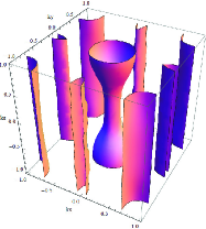
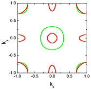
Figure 1: 3-D Fermi surfaces and Contour plot of Fermi surfaces in the extended three-band model Eq.(Inter-layer Superconducting Pairing Induced $c$-axis Nodal Lines in Iron-based Superconductors) ($k_{z}=0$ for the read line and $k_{z}=\pi$ for the green line).

The Hamiltonian of our model includes two parts $H=H_{t}+H_{I},$ where $H_{t}$ is the kinetic energy and $H_{I}$ is the pairing interaction. $H_{t}$ is given by

$$H_{t}=\sum_{\mathbf{k},\alpha\beta\sigma}\varepsilon_{\mathbf{k}\alpha\beta}d_{\mathbf{k}\alpha\sigma}^{{\dagger}}d_{\mathbf{k}\beta\sigma},$$

where $\alpha,\beta=1,2,3$ label the 3d electrons in the $d_{xz}$, $d_{yz}$ and $d_{z^{2}}$ orbital respectively. The form of the kinetic energy and the hopping parameters are constructed by extending the two-orbital model raghu to achieve the $c$-axis dispersion that matches well the experimental results. Their explicit forms are

$$\varepsilon_{\mathbf{k},11}=-2t_{1}\cos k_{x}-2t_{2}\cos k_{y}-4t_{3}\cos k_{x}\cos k_{y}-\mu,$$

$$\varepsilon_{\mathbf{k},22}=-2t_{2}\cos k_{x}-2t_{1}\cos k_{y}-4t_{3}\cos k_{x}\cos k_{y}-\mu,$$

$$\varepsilon_{\mathbf{k},33}=2t_{z}\left(\cos k_{x}+\cos k_{y}\right)-\mu_{3},$$

$$\varepsilon_{\mathbf{k},12}=-4t_{4}\sin k_{x}\sin k_{y},$$

$$\varepsilon_{\mathbf{k},13}=-t_{xz}\left(1-\cos k_{z}\right)\left(\cos k_{x}+\cos k_{y}\right)\sin k_{x},$$

$$\varepsilon_{\mathbf{k},23}=t_{xz}\left(1-\cos k_{z}\right)\left(\cos k_{x}+\cos k_{y}\right)\sin k_{y}.$$

The c-axis dispersion is induced by the coupling between the $d_{xz,yz}$ and $d_{z^{2}}$ orbitals. The later is taken to be below the Fermi level. In the explicit form of the coupling between these orbitals, $\varepsilon_{\mathbf{k},13}$, we have taken into account both the lattice symmetry requirements and the experimental observations. By taking the following parameters $t_{1}=-1,t_{2}=1.55,t_{3}=t_{4}=-0.85,t_{z}=1,t_{xz}=0.8,\mu=1.77,\mu_{3}=5$, we find that the model describes well the 3-dimensional Fermi surfaces measured experimentally dlfeng2010 ; dlfeng2011 as shown in Fig. 1.

$H_{I}$, the SC pairing interaction, generally includes the following terms,

$$H_{intra,1} = -V_{1}\sum_{\mathbf{kk^{\prime}},\alpha=1,2}\phi^{(1)}_{\mathbf{k}}\phi^{(1)}_{\mathbf{k^{\prime}}}d_{\mathbf{k}\alpha\uparrow}^{{\dagger}}d_{\mathbf{-k}\alpha\downarrow}^{{\dagger}}d_{\mathbf{-k^{\prime}}\alpha\downarrow}d_{\mathbf{k^{\prime}}\alpha\uparrow}$$

$$H_{inter,2} = -V_{2}\sum_{\mathbf{kk^{\prime}},\alpha=1,2}\phi^{(2)}_{\mathbf{k}}\phi^{(2)}_{\mathbf{k^{\prime}}}d_{\mathbf{k}\alpha\uparrow}^{{\dagger}}d_{\mathbf{-k}\alpha\downarrow}^{{\dagger}}d_{\mathbf{-k^{\prime}}\alpha\downarrow}d_{\mathbf{k^{\prime}}\alpha\uparrow}$$

$$H_{inter,3} = -V_{3}\sum_{\mathbf{kk^{\prime}}}\phi^{(3)}_{\mathbf{k}}\phi^{(3)}_{\mathbf{k^{\prime}}}d_{\mathbf{k},3\uparrow}^{{\dagger}}d_{\mathbf{-k},3\downarrow}^{{\dagger}}d_{\mathbf{-k^{\prime}},3\downarrow}d_{\mathbf{k^{\prime}},3\uparrow}$$

$$H_{inter,4} = -V_{4}\sum_{\mathbf{kk^{\prime}}}\phi^{(4)}_{\mathbf{k}}\phi^{(4)}_{\mathbf{k^{\prime}}}(d_{\mathbf{k},1\uparrow}^{{\dagger}}d_{\mathbf{-k},1\downarrow}^{{\dagger}}d_{\mathbf{-k^{\prime}},3\downarrow}d_{\mathbf{k^{\prime}},3\uparrow}$$

$$+d_{\mathbf{k},2\uparrow}^{{\dagger}}d_{\mathbf{-k},2\downarrow}^{{\dagger}}d_{\mathbf{-k^{\prime}},3\downarrow}d_{\mathbf{k^{\prime}},3\uparrow}+h.c.).$$

The first term $H_{intra,1}$ describes the intra-layer pairing while the rest three terms describe the different inter-layer pairing interactions. $H_{inter,2}$ accounts for the inter-layer pairing interaction between the $d_{xz}$ and $d_{yz}$ orbitals, as does $H_{inter,3}$ for the $d_{z^{2}}$ orbital. The last term describes the inter-layer interaction between the $d_{z^{2}}$ and $d_{xz,yz}$ pairs. We take $\phi^{(1)}_{\mathbf{k}}$ to be the intra-layer $S^{\pm}$-wave paring function $\phi^{(1)}_{\mathbf{k}}=\cos k_{x}\cos k_{y}$ and $\phi^{(2)}_{\mathbf{k}}=(\cos k_{x}+\cos k_{y})\cos k_{z}$, and $\phi^{(3,4)}_{\mathbf{k}}=\cos k_{z}$. These choices rely on the assumption that the SC pairing in iron-based superconductors is rather short-ranged. The form of $\phi^{(1)}$ has been proposed in the models based on local magnetic exchange couplings seo2008 ; Fang2011 ; huj ; Yu2011 and it has been shown that the form factor is consistent with current experimental results nodeless1 . The form of $\phi^{(2)}$ has been proposed in hding , which can be obtained from the existence of AFM exchange couplings between the layers daipc ; daipc2 . The form of $\phi^{(3,4)}$ and the corresponding $V_{3,4}$ pairing interactions can be understood as the inter-layer pairing is between two adjacent layers and the pairing symmetry is s-wave. $V_{3}$ describes the inter-layer pairing for the $d_{z^{2}}$ orbital. The $V_{4}$ term, which describes the coupling between two inter-layer pairings of two different orbitals, can be understood in the following way. Since the c-axis hopping term in $H_{t}$ describes the hopping between two adjacent layers and the $d_{z^{2}}$ is below the Fermi level, the second order perturbation through such hopping would generically produce $V_{4}\propto\frac{t_{xz}^{2}}{\mu_{3}}$.

In the self-consistent mean-field theory for the SC state, $H_{I}$ becomes

$$H_{BCS}=-\sum_{\mathbf{k}\alpha}\Delta_{\alpha}(\mathbf{k})d_{\mathbf{k}\alpha\uparrow}^{{\dagger}}d_{\mathbf{-k}\alpha\downarrow}^{{\dagger}}+h.c.,$$ (1)

where $\Delta_{1}(\mathbf{k})=\Delta^{(1)}_{1}\phi^{(1)}_{\mathbf{k}}+\Delta^{(2)}_{1}\phi^{(2)}_{\mathbf{k}}+\Delta^{(4)}_{3}\phi^{(4)}_{\mathbf{k}}$, $\Delta_{2}(\mathbf{k})=\Delta^{(1)}_{2}\phi^{(1)}_{\mathbf{k}}+\Delta^{(2)}_{2}\phi^{(2)}_{\mathbf{k}}+\Delta^{(4)}_{3}\phi^{(4)}_{\mathbf{k}}$ and $\Delta_{3}(\mathbf{k})=\Delta^{(3)}_{3}\phi^{(3)}_{\mathbf{k}}+(\Delta^{(4)}_{1}+\Delta^{(4)}_{2})\phi^{(4)}_{\mathbf{k}}$. Here $\Delta^{(n)}_{\alpha}$ is defined by

$$\Delta^{(n)}_{\alpha}=V_{n}\sum_{\mathbf{k}}\phi^{(n)}_{\mathbf{k}}\langle d_{\mathbf{-k}\alpha\downarrow}d_{\mathbf{k}\alpha\uparrow}\rangle.$$ (2)

Results Before we present a full numerical solution for the above Hamiltonian, we first discuss the simple physical picture for the generation of the nodal points in the gap function on the hole pocket. In the above model, if we consider the general intra-orbital pairing form of the $d_{xz,yz}$ orbitals, the $k_{z}$-dependent SC gap can be written as

$$\Delta(\mathbf{k})=\Delta_{0}\left[\cos k_{x}\cos k_{y}+\delta_{z}\left(\lambda+\cos k_{x}+\cos k_{y}\right)\cos k_{z}\right],$$ (3)

where the first term represents the $S^{\pm}$ pairing and the second term represents the inter-layer pairing with the $S$-wave pairing symmetry. In the first order approximation, this intra-orbital pairing roughly determines the SC gap since it dominates as we will show later. This form indicates that the inter-layer pairing is between the two neighboring layers. The gap zero points develop as $\delta_{z}$ increases. As shown in Fig. 2, when $\delta_{z}$ reaches a certain value, the contour of the gap zeroes will cross the Fermi surface at the points near $k_{z}=\pm\pi$, which leads to the nodal behavior.

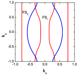
Figure 2: A cartoon plot for the gap nodal picture in the momentum space $(k_{x},0,k_{z})$. The blue lines are the contour lines for zero gap value of Eq. (3) with $\delta_{z}=0.4$ and $\lambda=0$. FS₁ and FS₂ are defined in Fig. 1. The intercept between the blue and the red lines produce the nodes in the hole pocket.

Second, we discuss two important, general results obtained from our model, which are independent of the detailed pairing interaction parameters $V_{i}$ in $H_{I}$. One of these is that the inter-layer pairing always competes with the intra-layer pairing. To demonstrate this more clearly, we switch off $V_{3}$ and $V_{4}$ and perform a self-consistent solution with $V_{1}$ and $V_{2}$. The SC pairing gaps as a function of the interacting parameters are shown in Fig.3. It is very clear that the intra-layer pairing reduces while the inter-layer pairing increases and vice versa. If we turn on all of the inter-layer pairing interactions, the results are rather similar: while the different inter-layer pairings can increase simultaneously, the intra-layer pairing gaps always decrease as the inter-layer ones increase. A typical result is presented in Fig.4. This result qualitatively suggests that a more quasi two-dimensional SC state is likely better for achieving a higher $T_{c}$ since the intra-layer pairing would dominate. So far the highest $T_{c}$ in the iron-based superconductors is achieved in the 1111-family. The highest $T_{c}$ in the 122 family is about 8 degrees lower than the one in the 1111-family johnston . Comparing to the 122 family, the 1111 family is much more two-dimensional with much less dispersion along the c-axis.

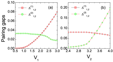
Figure 3: Gaps versus pairing interactions. Interaction parameters in (a) are defined as $V_{2}=3,V_{3}=V_{4}=0$ and (b) $V_{1}=3,V_{3}=V_{4}=0$. $\Delta^{(n)}_{\alpha}$ is defined in Eq. (2).

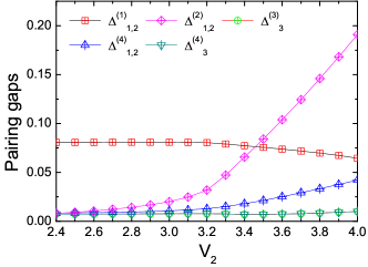
Figure 4: Gaps versus pairing interaction $V_{2}$ with $V_{1}=V_{3}=V_{4}=3$.

In a multi-orbital model, the relation between the SC pairing parameters and the energy gap in the low energy single particle excitations can be complicated. In order to show that the SC state truly develops nodes, we have to calculate the energy dispersion of the Bogoliubov quasiparticles at the Fermi surfaces. In Fig.5, we plot the dispersion of Bogoliubov quasiparticles along the c-axis with the parameters given by $V_{1}=3,V_{2}=3.35,V_{3}=V_{4}=3$. There are two important results. One is that the true nodes can easily develop on the hole pocket. The other is that the gap values of the quasiparticles on the hole pocket and electron pocket are anti-correlated along the c-axis: the gap value on the hole pocket is larger at $k_{z}=0$ than at $k_{z}=\pi$ while on the electron pocket, it is smaller at $k_{z}=0$ than at $k_{z}=\pi$. This anti-correlation is a combined result of the inter-layer pairing and the $S^{\pm}$-wave symmetry for the intra-layer SC pairing order parameter which is proportional to $cosk_{x}cosk_{y}$ and changes sign between the hole and the electron pocket. This result holds for most of the parameter regions we have investigated. Therefore, this inter-layer pairing induced anti-correlation suggests that ARPES can provide a direct test of the possible $S^{\pm}$-wave pairing gap functions in the iron-pnicitide superconductors. Of course, to detect it, a high energy-resolution in the ARPES experiments has to be achieved since the c-axis dispersion and the gap modulation on the electron pockets are not large.

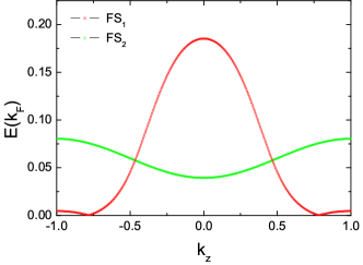
Figure 5: The energy dispersion of the Bogoliubov quasiparticles at the Fermi surfaces shown in Fig. 1. Here $V_{1}=3,V_{2}=3.35,V_{3}=V_{4}=3$ with $\Delta^{(1)}_{1,2}=0.078,\Delta^{(2)}_{1,2}=0.057,\Delta^{(3)}_{3}=0.007,\Delta^{(4)}_{1,2}=0.016,\Delta^{(4)}_{3}=0.007$.

Finally, we note that several previous thermal conductivity measurements have suggested that the nodes should be on the electron pockets linenode2 . A key argument given in linenode2 is that the quaisparticles on the hole pockets have much lower velocity and heavier mass than those on the electron pockets so that the in-plane Fermi velocity $V_{F}$ of the hole pockets is too small to explain the observed residual thermal conductivity. However, this statement is only partially true. There are three hole pockets centered around the folded Brillouin zone center. The Fermi velocity on one of the hole pockets is in fact comparable to that on the electron pockets. ARPES results hdingtwo show that the former is even slightly larger than the later. This hole pocket, whose orbital character is even with respect to the $\Gamma-M$ mirror plane, is exactly the pocket that carries the large c-axis dispersion. Therefore, the previous thermal conductivity measurements are consistent with our results for the existence of gap nodes on the hole pocket.

Conclusion We have constructed a model to show how nodes in the single-particle excitations can emerge in iron-based superconductors. The development of the nodes are due to the combined effects of the increase in the hole pocket size which reduces the SC gap from intra-layer pairing and the presence of the inter-layer SC pairing. This study consistently explains the experimental observations of the c-axis gap variation in optimally hole-doped $Ba_{1-x}K_{x}Fe_{2}As_{2}$ ZhangBK ; hding and the nodal behaviors in $BaFe_{2}As_{2-x}P_{x}$ dlfeng2011 . We also demonstrated that the inter-layer and intra-layer pairing generally competes with each other, and suggested a direct experimental test of the $S^{\pm}$-wave pairing symmetry through the anti-correlation of the gap modulations on the hole and electron pockets that can be measured by ARPES. We believe that our results can also explain the observed nodal behaviors in other materials such as $KFe_{2}As_{2}$ and $AFe_{2-x}Ru_{x}As_{2}$. A concrete test of our model will be whether the gap functions observed in these materials obey Eq. (3) as the leading contribution to the quasi-3D SC pairing gap function.

Acknowledgement: We thank H. Ding, D. L. Feng, P. C. Dai, N. L. Wang, H. H. Wen and C. Fang for useful discussions. Y.H. is supported by the NSFC (No. 10974167). ZW is supported by DOE DE-FG02-99ER45747.

References

- (1) Kamihara, Y., Watanabe, T., Hirano, M. & Hosono, H. J. Am. Chem. Soc. 130, 3296, (2008).
- (2) For a review, Johnston D. Adv. Phys. 59, 803, 2010.
- (3) For a review, Hirschfeld, P. J., Korshunov M. M. and Mazin I. I. Arxiv:1106.3712 (2011).
- (4) Seo, K., Bernevig B. A., and Hu J., Phys. Rev. Lett. 101, 206404 (2008).
- (5) Fang C., et al, Phys. Rev. X 1, (2011).
- (6) Hu, J. and Ding, H. arXiv:1107.1334 (2011)
- (7) Yu R., et al. arXiv:1103.3259 (2011).
- (8) Mazin, I. I. et al. Phys. Rev. Lett. 101, 057003 (2008).
- (9) Kuroki, K. et al. Phys. Rev. Lett. 101, 087004 (2008).
- (10) Wang, F. et al. Phys. Rev. Lett. 102, 047005 (2009).
- (11) Ding, H. et al. Europhys. Lett. 83, 47001 (2008).
- (12) Zhang Y., et al, Nature Materials (2010).
- (13) Hanaguri, T. et al. Science, 328 474 (2010).
- (14) Hashimoto, K. et al. Phys. Rev. B 81, 220501 (2010).
- (15) Yamashita, M. et al., arXiv:1103.0885 (2011).
- (16) Nakai, Y. et al. Phys. Rev. B 81, 020503 (2010).
- (17) Cheng B. et al. Phys. Rev. B 83, 144522 (2011).
- (18) Zeng B., et al, Nature Communications 1, 112 (2010).
- (19) Qiu, X, et al, arXiv:1106.5417 (2011).
- (20) Shuai, J. et al. J. Phys.: Condens. Matter 21, 382203 (2009).
- (21) Shishido, H. et al. Phys. Rev. Lett. 104, 057008 (2010).
- (22) Shuai, J. et al. J. Phys.: Condens. Matter 21, 382203 (2009).
- (23) Wang, C. et al. Europhys. Lett. 86 47002 (2009).
- (24) Zhang, Y. et al. arXiv:1109.0229 (2011).
- (25) Ye Z.R. et al. arXiv:1105.5242 (2011).
- (26) Kuroki, K., et al. Phys. Rev. B 79, 224511 (2009).
- (27) Wang, F., Zhai, H. & Lee, D.-H. Phys. Rev. B 81, 184512 (2010).
- (28) Thomale, R.,et al. Phys. Rev. Lett. 106, 187003 (2011).
- (29) Suzuki, K., Usui, H. & Kuroki, K. J. Phys. Soc. Jpn. 80 (2011).
- (30) Zhang, Y. et al. arXiv:1109.0229 (2011).
- (31) Zhang, Y. et al. Phys. Rev. Lett. 105, 117003 (2010).
- (32) Xu, Y.M., et al, Nature Physics, 7, 198 (2011).
- (33) Yuan, H. Q. et al, Nature, 457, 565 (2009).
- (34) Ren Z. et al, Chin. Phys. Lett 25, 2215 (2008).
- (35) Chen X.H. et al, Nature 453, 761 (2008).
- (36) Zhang Y. et al, Phys. Rev. B 83, 054510 (2011).
- (37) Chi S. et al, Phys. Rev. Lett 102, 107006 (2009).
- (38) Wang G. et al, Phys. Rev. Lett 104, 047002 (2010).
- (39) Zhao J. et al, Nature Physics 5, 555 (2009).
- (40) Zhao J. et al, Phys. Rev. Lett. 101, 167203 (2008).
- (41) Zhang Y. et al, Phys. Rev. B 83, 054510 (2011).
- (42) Raghu S. et al, Phys. Rev. B 77, 220503 (2008).
- (43) Ding H. et al, J. Phys. Cond. Matt. 23, 135701 (2011).