Interplay between hydrodynamics and the free energy surface in the assembly of nanoscale hydrophobes

Abstract

Solvent plays an important role in the relative motion of nanoscopic bodies, and the study of such phenomena can help elucidate the mechanism of hydrophobic assembly, as well as the influence of solvent-mediated effects on in vivo motion in crowded cellular environments. Here we study important aspects of this problem within the framework of Brownian dynamics. We compute the free energy surface that the Brownian particles experience and their hydrodynamic interactions from molecular dynamics simulations in explicit solvent. We find that molecular scale effects dominate at short distances, thus giving rise to deviations from the predictions of continuum hydrodynamic theory. Drying phenomena, solvent layering, and fluctuations engender distinct signatures of the molecular scale. The rate of assembly in the diffusion-controlled limit is found to decrease from molecular scale hydrodynamic interactions, in opposition to the free energy driving force for hydrophobic assembly, and act to reinforce the influence of the free energy surface on the association of more hydrophilic bodies.

I Introduction

The hydrophobic effect plays a fundamental role in biology and nanoscale engineering. Great strides have been made in our understanding of the mechanism of hydrophobic assembly by elucidating the behavior of solvent near interfaces of variable length scale. Pangali et al. (1979); Chandler (2005); Berne et al. (2009); Jamadagni et al. (2011); Wallqvist and Berne (1995); Hummer et al. (1996); Lum et al. (1999); Huang and Chandler (2002); Ten Wolde and Chandler (2002); Huang et al. (2003); Zhou et al. (2004); Huang et al. (2005); Giovambattista et al. (2007); Mittal and Hummer (2008); Willard and Chandler (2008); Sarupria and Garde (2009); Godawat et al. (2009); Patel et al. (2010) In addition, the hydrophobic effect is crucial to understanding the nature of surface friction in nanoscale fluid transport. Huang et al. (2008); Sendner et al. (2009); Thomas and McGaughey (2009); Kalra et al. (2010); Falk et al. (2010); Bocquet and Charlaix (2010) Surface friction characterizes the boundary condition in the continuum description for fluid flow across interfaces of varying hydrophobicity.

Despite recent efforts to improve our understanding of the hydrophobic effect, to our knowledge the role of hydrodynamic interactions in hydrophobic assembly has not been considered. Within the framework of Brownian dynamics, hydrodynamic interactions are incorporated in the frictional force by means of a resistance (friction) tensor that is dependent upon the degrees of freedom of the Brownian bodies. Ermak and McCammon (1978) Hydrodynamic interactions are typically treated in the simulation of colloidal suspensions within the continuum description of low Reynolds number flow. Brady et al. (1988); Brady (1988); Chatterji and Horbach (2005); Padding and Louis (2006) Recently, polydisperse colloidal simulations intended to mimic cytoplasm reported that hydrodynamic interactions give rise to the slow diffusion of macromolecules observed in crowded cellular environments. Ando and Skolnick (2010)

For small separations, the continuum description is dominated by lubrication effects, which yields a friction constant that diverges as two bodies come into contact. Such frictional forces arise from the assumption that there is a fluid element present even as the spacing approaches zero. Naturally, this description breaks down when molecular scale effects become important at small length scales. The continuum description of the Navier-Stokes equation is expected be valid down to length scales of approximately $1-2$ nm. Thomas and McGaughey (2009); Bocquet and Charlaix (2010) Therefore, molecular-scale effects should be considered when only a few solvent layers separate the solute.

The spatially dependent friction tensor can be extracted from explicit molecular dynamics simulations where all bath degrees of freedom are included. This may be achieved in either the Brownian limit or when memory effects are included. Berne and Harp (1970); Straub et al. (1987, 1990); Español and Zúñiga (1993); Bocquet et al. (1994, 1997) To our knowledge, the friction tensor between two bodies has only been previously computed in Lennard-Jones fluids. Straub et al. (1990); Bocquet et al. (1997); Lee (2010) Presently we consider the spatial dependence of the friction constant as function of the distance between two non-polar spherical bodies in explicit water. The spatial friction, in concert with the (non-hydrodynamic) potential of mean force along the relative direction, facilitates the modeling of two-body assembly in the Brownian limit and an assessment of the importance of hydrodynamic and non-hydrodynamic forces.

This work aims to elucidate the role that hydrodynamics plays in hydrophobic assembly. We take as our model solute two fullerenes, either two C60s or two C240s. Unsubstituted fullerenes are insoluble in water, Bezmel’nitsyn et al. (1998) and thus, to our knowledge there are no experimental data on their transport in water. Nevertheless they are a useful model for theoretically probing the transport of nanoscale bodies. The hydrophobic collapse of two bodies in explicit water Huang et al. (2003, 2005) and pathways for self-assembly of hydrophobic spheres in a coarse grained solvent model Willard and Chandler (2008); Ten Wolde and Chandler (2002) have been previously studied. The potential of mean force of two C60 molecules in water has also been computed. Hotta et al. (2005); Makowski et al. (2009) However, the interplay between the free energy surface and hydrodynamic interactions has not yet been considered. As we will show, solvent fluctuations and drying phenomena manifest themselves as hydrodynamic interactions within the Brownian framework. We find that because slow relaxation times are associated with the solvent at the drying transition the separation of solute and solvent time scales required by a Brownian description of hydrophobic assembly may not always be satisfied.

The solute-solvent interactions are described by both attractive and purely repulsive potentials. For the purely repulsive model of the fullerene we observe a drying transition, Wallqvist and Berne (1995) one which is more pronounced for C240 than C60, a finding which is in agreement with the known length-scale dependence of drying phenomena. Lum et al. (1999); Huang et al. (2003) The attractive spheres do not dry as they approach each other and water is expelled from the inter-solute region by means of steric repulsion. We find that the spatial dependence of the friction constant is quite different in each of these cases. In particular, drying phenomena and solvent layering engendered by attractive potentials are shown to possess distinct signatures in their respective friction tensor. Hydrodynamic interactions at the molecular scale are related to the variability of solvent density, fluctuations, and relaxation times in the inter-solute region as two bodies approach.

The rate constant for assembly is computed via a Smoluchowski Analysis. Emeis and Fehder (1970); Deutch and Felderhof (1973); Wolynes and Deutch (1976); Northrup and Hynes (1979); Calef and Deutch (1983); Straub et al. (1990) We find that for two body assembly, the inclusion of hydrodynamic interactions decreases the rate of reaction in the diffusion controlled limit by approximately $30-40\%$. In the case of ideal hydrophobic assembly (that is when no solute-solvent attraction is present) the frictional and mean force can be said to have opposite effects. When solute-solvent attraction is included, they tend to reinforce each ether’s impact on the rate of assembly.

This paper is organized as follows. Sec. II reviews the formalism of hydrodynamic interactions and Brownian motion. Simulation details are given in Sec. III. Results are given for the friction coefficient on a single body in Sec. IV and are compared with the Stokes-Einstein relation with periodic boundary corrections. In Sec. V an analysis of the assembly of two non-polar solutes within the framework of Brownian motion is presented. Discussions and conclusions are given in Sec. VI.

II Langevin dynamics and hydrodynamic interactions

In this work we seek to characterize solvent-mediated effects on two spherical bodies. The Brownian limit is considered such that the bodies evolve on a much slower time scale than the solvent bath. The dynamics of such a system can be described by an equation of motion that includes contributions from three forces, a frictional force, a mean force, and an uncorrelated, Gaussian random force. Due to the symmetry of the problem, the relative distance $r=\left|\vec{r}_{2}-\vec{r}_{1}\right|$ between the spheres is the only coordinate necessary to characterize the approach of the two solute bodies. In the present study we concentrate on this direction, and will consider the friction along other degrees of freedom in future work. When hydrodynamic interactions are included in the frictional force, the Langevin equation for the motion of the relative coordinate is given by, Ermak and McCammon (1978)

$$\mu\ddot{r} =-\nabla\mathcal{W}(r)-\zeta(r)\dot{r}+R(r,t)\;,$$ (1)

where $\mu$ is the reduced mass and $\mathcal{W}(r)$ is the potential of mean force. In the Brownian limit the solvent (hydrodynamic) time scale is separable from the motion of the solute and so the friction tensor may be computed at fixed solute positions. Dhont (1996) This is analogous to the Born-Oppenheimer approximation, which assumes a similar separation of time scales between nuclear and electronic degrees of freedom. The (non-hydrodynamic) free energy profile contains contributions from both direct solute-solute interactions and induced solvent-mediated forces. In the limit of large friction the term on the left-hand side of Eqn. 1 may be neglected. The friction coefficient $\zeta(r)$ can be determined from the full two-body tensor as reviewed in the Appendix. The random force, $R(r,t)$, is Gaussian, uncorrelated noise with zero mean and a variance that is related to the friction coefficient via the fluctuation-dissipation theorem,

$$\left<R(r,t)R(r,0)\right> =2k_{b}T\zeta(r)\delta(t)\;.$$ (2)

As indicated by Eqn. 1, when hydrodynamic interactions are included the friction coefficient depends on the distance between spheres. If hydrodynamic interactions are ignored then $\zeta(r)\rightarrow\zeta_{0}$, where $\zeta_{0}$ is taken to be the friction coefficient on the relative coordinate at infinite separation where no spatial dependence is assumed.

Hydrodynamic interactions that yield the spatial dependence of the friction coefficient are typically computed by means of approximate solutions of the linearized Navier-Stokes equation valid for incompressible flow at low Reynolds number. A ubiquitous formulation of hydrodynamics frequently utilized in colloidal simulations is Stokesian dynamics. Brady et al. (1988); Brady (1988) Stokesian dynamics interpolates between an exact two-body solution for short range interactions Jeffrey and Onishi (1984) and the long range many-body result derived from the Rotne-Prager tensor as applied to systems with periodic boundary conditions. Beenakker (1986). Other techniques may also be utilized to compute continuum hydrodynamic interactions Chen (1998); Chatterji and Horbach (2005); Padding and Louis (2006); Nakayama et al. (2008) and the continuum formulation has been recently employed as a framework for coarse-grained solvent models. Voulgarakis and Chu (2009) In this work we will compare our molecular scale results to both the expression of Ref. Jeffrey and Onishi, 1984 and the Oseen tensor computed with periodic boundary conditions. Hasimoto (1959); Lindbo and Tornberg (2010) The Oseen tensor is the leading order term of the Rotne-Prager expression Dhont (1996).

The continuum approach breaks down for small particle separations, and in this work we seek to determine hydrodynamic interactions at the molecular scale. The solvent bath is treated by explicit Newtonian (microcanonical) molecular dynamics simulation. All bath degrees of freedom and microscopic details are present in our simulation. The friction coefficient is related to the microscopic fluctuations in the linear response regime by means of a Green-Kubo relation. This equates the friction tensor to the correlation function of the fluctuations of the total force on each Brownian body, $\delta F_{i}=F_{i}-\left<F_{i}\right>$. Berne and Pecora (1990).

$$\mathrm{\underline{\underline{\zeta}}}_{ij}=\frac{1}{k_{b}T}\int\limits_{0}^{\infty}\mathrm{d}t\;\lim\limits_{N\rightarrow\infty}\left<\delta\vec{F}_{i}(t)\delta\vec{F}_{j}(0)\right>$$ (3)

Where $\zeta_{ij}$ is a component of the friction tensor (see Appendix). Unfortunately, this formula may only be directly applied in both the Brownian limit ($M_{\mathrm{solute}}\rightarrow\infty$) and in the thermodynamic limit where the number of solvent molecules, $N$, approaches infinity. Berne and Pecora (1990); Bocquet et al. (1994, 1997). Although the former requirement may be satisfied by fixing the positions of the Brownian particles, the latter requirement gives rise to subtle complications in a finite simulation. Utilizing the techniques developed by Bocquet et Ab. Eqn. 3 may be employed to indirectly compute the two-body friction coefficient, that is the MD estimate of $\mathrm{\underline{\underline{\zeta}}}_{ij}$ can be related to linear combinations of the submatricies of the friction tensor. Bocquet et al. (1997) Similar complications are present in the computation of the friction on a single body. Bocquet et al. (1994) Further details are provided in the Appendix.

III System setup and simulation details

In order to gauge the impact of size effects, we utilize two fullerenes, C60 and C240, as our model non-polar bodies. The two molecules and their relative sizes are depicted in panel (b) of Fig. 1. The solute-solvent interactions are described by two forms, a Lennard-Jones (LJ) interaction with parameters $\sigma_{\text{SS}}=0.332\text{ nm}$ and $\epsilon_{\text{SS}}=0.423\text{ kJ/mol}$, and a Weeks-Chandler-Andersen (WCA) truncation of this potential Weeks et al. (1971). As will be shown below, there is vastly different behavior when the potential is attractive or purely repulsive. For the purpose of the friction analysis the fullerenes are treated as spheres and the friction coefficient is computed on their respective centers of mass. Based on the choice of repulsive core, the estimated Van der Waals diameters for C60 and C240 are $\sigma=1.0$ nm and $\sigma=1.7$ nm, respectively.

The friction is sensitive to periodic boundary conditions (see Sec. IV), and we utilize as large a system as is computationally feasible. For runs containing C60 the base box length prior to equilibration is 5.0 nm and for C240 it is 6.0 nm. In systems containing two fullerenes, a set of calculations was run with the bodies frozen and set at a fixed distance apart from each other. The box length is extended by the separation between solute centers of mass in the axial direction of the starting configuration of each computation. The number of water molecules utilized to represent the solvent varies between approximately $5000-11000$ depending on the size of the fullerene and the size of the separation. Water is modeled with the TIP4P potential Jorgensen and Madura (1985). Snapshots Humphrey et al. (1996) of two C240 molecules fixed at three different separations are shown in Fig. 2. Each system was equilibrated under NPT conditions for 2 ns and NVT conditions for 1 ns. The barostat of Berendsen Berendsen et al. (1984) and a stochastic velocity rescaling thermostat Bussi et al. (2007) were employed during equilibration runs to maintain a temperature of 300 K and a pressure of 1 bar. In order to compute the friction coefficient, data was collected from $10-18$ NVE runs of 4 ns in length at each fixed distance. All calculations were performed using GROMACS version 4.5.3. Hess et al. (2008) As the friction is a probe of the solvent momentum relaxation in the presence of the solute bodies, its computation requires strict energy conservation in the microcanonical ensemble. NVE runs were performed in double precision.

The computation of the spatially dependent friction coefficient requires constant energy simulations and three dimensional periodic boundary conditions are necessary for comparison with long range periodic continuum hydrodynamics. Therefore, behavior at the drying transition must be studied at constant volume and in the absence of an interface. The number of solvent molecules we choose is large enough to accommodate the study of a dewetting transition and although the behavior is modestly perturbed by this choice of ensemble, the qualitative features of the friction at the critical distance for dewetting are not expected to suffer. As the two solutes are fixed throughout all computations, direct solute-solute interactions are not a component of the simulations described above. Direct interactions between fullerenes are included in the computation of the rate constant in Sec. V.3 and the solute-solute potential has the parameters $\sigma=0.35\;\text{nm}$ and $\epsilon=0.276\;\text{kJ/mol}$.

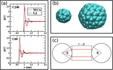
Figure 1: (a) The pair-correlation function from the center of C240 (top panel) or C60 (bottom panel) to the oxygen site on the water molecule is depicted for the cases when the solute-solvent potential is purely repulsive (dashed black curve) or includes attraction (solid red curve). (b) The two fullerenes utilized to model non-polar spherical bodies, C60 (left) and C240 (right) are visualized with VMD. Humphrey et al. (1996) The estimated diameter for each species is 1.0 nm and 1.7 nm, respectively. (c) Two spherical bodies of diameter $\sigma$ are placed a distance $r$ from each center. A cylindrical probe volume (blue lines) is chosen such that its length is $r-\sigma$ and its diameter determined by the angle $\phi=90^{\circ}$. This volume can be further partitioned into an inner-tube (red lines) whose diameter is determined by the angle $\theta=60^{\circ}$ and an outer shell that is the difference between the two probe volumes.

IV Friction on a fullerene in solvent

The strength of non-polar attractions play an important role in the degree of particle hydrophobicity (see e.g. Ref. Huang and Chandler, 2002). This is readily seen in panel (a) of Fig. 1, where the pair correlation function of the solvent with respect to the center of mass of the fullerene is plotted. Whereas the attractive fullerenes exhibit significant structuring of the first solvation shell, the water density is depleted near the surface of the repulsive bodies. The pair correlation function for C60 is in good agreement with previous studies of hydration around fullerenes. Weiss et al. (2008) Furthermore, depletion becomes more prominent with increasing solute size, a finding that is in agreement with prior theoretical predictions and simulation. Lum et al. (1999); Mittal and Hummer (2008)

The friction coefficient of a single C60 and C240 molecule is computed utilizing both the LJ and WCA solute-solvent potentials. These values may be related to the Stokes radius via the Stokes-Einstein relation corrected for periodic boundary conditions (PBC). Hasimoto (1959); Yeh and Hummer (2004) As noted in the cited works, PBC have a large impact on the measured friction. To leading order this correction, as formulated in Ref. Yeh and Hummer, 2004, is given by the following expression,

$$\frac{1}{\zeta_{\text{iso}}}=\frac{1}{\zeta_{\text{PBC}}}+\frac{\xi}{6\pi\eta L}\;\;,$$ (4)

where $\xi=2.837297$, $L$ is the periodic box length, and $\eta$ is the shear viscosity. The value of the viscosity of the TIP4P model used in this work has been taken from the literature. Gonzalez and Abascale (2010)

Once the friction coefficient of the isolated sphere, $\zeta_{\text{iso}}$, has been computed, it can be related to the Stokes radius, which is given by,

$$r_{\text{stokes}} =\frac{\zeta_{\text{iso}}}{c\pi\eta}\;\;,$$ (5)

where $c$ is equal to $4$ or $6$ for slip or stick boundaries, respectively. Studies relating Eqn. 5 to the results of molecular dynamics simulation have appeared in the literature Schmidt and Skinner (2003, 2004); Li (2009) and subtleties associated with the appropriate hydrodynamic radius and boundary choice should be addressed for a complete understanding of how this continuum expression applies at the molecular scale. Furthermore, we note that if our model solutes were perfect spheres (which they are not), then the slip boundary condition holds unless solute-solvent attractions are so large that solvent molecules become entrenched on the surface. Schmidt and Skinner (2004) Presently, we simply assume either a stick or slip boundary condition and compute the stokes radii of the fullerenes with the LJ and WCA solute-solvent potentials. The results are presented in Table 1 and compared with the estimated van der Waals radii. One can see that the stokes radii of the purely repulsive spheres with slip boundary conditions are in very good correspondence with the van der Waals radii. As the molecules become more attractive, the friction coefficient increases as does in this sense the “stickiness” of the surface. This is in agreement with studies of water at interfaces, which have shown that there is a correlation between hydrophobicity and the friction tangential to the surface. Huang et al. (2008); Sendner et al. (2009) Furthermore, studies of particle diffusion in a Lennard-Jones fluid have exhibited similar trends as a function of solute-solvent attraction. Schmidt and Skinner (2004); Li (2009)

In the following analysis, we determine the friction coefficient along the relative coordinate in units of $\zeta_{0}=\zeta_{\text{PBC}}/2$ for each respective fullerene and solute-solvent potential. The two body simulations utilize a periodic box of dimensions $(L+d)\times L\times L$ and therefore this choice accounts for the impact of periodic conditions. Changes relative to $\zeta_{0}$ are a result of hydrodynamic interactions and not PBC artifacts.

		Stokes radius (slip)	Stokes radius (stick)	Estimated vdW radius
C60	WCA	0.53 nm	0.35 nm	0.50 nm
C60	LJ	0.66 nm	0.44 nm	0.50 nm
C240	WCA	0.84 nm	0.56 nm	0.85 nm
C240	LJ	1.06 nm	0.70 nm	0.85 nm

Table 1: Table of computed Stokes radii for C60 and C240 with differing solute-solvent interactions.

V Two-body relative friction

The friction coefficient on the relative coordinate has been computed as a function of the distance between two spherical bodies where the solute-solvent interaction is either attractive or purely repulsive. We find starkly different behavior in each case, as will be discussed below. In both cases, there is significant deviation from continuum hydrodynamic predictions at small separations. In Fig. 2 we plot the relative friction coefficient as a function of the sphere separation $r-\sigma$ for C240 where solute-solvent interactions are purely repulsive or include attraction. Two expressions from continuum hydrodynamics, the two-body result valid at small separations and the result of the Oseen tensor corrected for periodic boundary conditions that is valid at long range, are also plotted. Jeffrey and Onishi (1984); Hasimoto (1959); Lindbo and Tornberg (2010); Nakayama et al. (2008) One can see that although the friction coefficient for $r-\sigma>1\text{ nm}$, approaches the long-range continuum result, the short-range value does not diverge at the point of contact as predicted by the expression of Ref. Jeffrey and Onishi, 1984. Instead, the frictional profile exhibits distinctive features of molecular-scale effects. For purely repulsive bodies, the friction coefficient peaks at a distance that corresponds to the critical distance for drying (see Sec. V.1). This distance increases with solute length scale Huang et al. (2003) and such drying phenomena is not encompassed by continuum hydrodynamics. In the case of bodies that strongly attract solvent, drying does not occur, and water is expelled by steric repulsion. This result is dependent upon the chosen value of $\epsilon_{SS}$. More weakly attractive spheres can exhibit dewetting. As discussed in Sec. V.2, distinctive molecular-scale behavior in which the friction coefficient exhibits signatures of solvent layering is observed as solvent is expelled from the inter-solute region. Furthermore, we note that the value of the long-range molecular scale results plotted in Fig. 2 appear to approach the description given by the periodic Oseen tensor. However, data points at larger separations would be necessary to make more definitive comparisons.

The occupancy and fluctuations of solvent molecules in a particular region of space may be monitored in a probe volume. This technique is a standard tool to study the hydrophobic effect (see e.g. Ref. Jamadagni et al., 2011). Nested cylindrical probe volumes are presently employed to study the water density and fluctuations in the inter-solute region. The probe cylinder is partitioned into an outer shell and an inner-tube. Due to the curvature of the hydrophobic surfaces, the density may be significantly different in the two shells, a finding that is particularly true in the case of the fullerenes which attract solvent. A diagram of the boundaries of the probe volume is sketched out in panel (c) of Fig. 1. The length of the cylinder is determined by the separation of the surfaces of bodies. The diameter of the cylinder is formed by a line tangent to the effective spherical surface of the fullerene and opposite an angle of $90^{\circ}$. The inner-tube is bounded in the same fashion except the angle opposite the tangent segment is $60^{\circ}$.

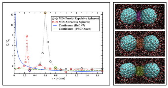
Figure 2: The friction coefficient is plotted as a function of the distance between two C240 molecules when the WCA potential and LJ potential is utilized to model solvent-solute interactions (black dotted line with circles and red dashed line with squares, respectively). The two-body (continuum) hydrodynamics result of Ref. Jeffrey and Onishi, 1984 (solid blue line) and the periodic Oseen tensor (dashed green line) are plotted against the molecular-scale computation. The three right-hand panels depict snapshots at separations (increasing from top to bottom) where, in the case of the WCA spheres, the inter-solute region is dry and the friction coefficient is low (violet circle), at the dewetting transition where the friction peaks coefficient (orange circle), and for large distances where the friction coefficient decays towards the baseline result (green circle). Water molecules within $0.6$ nm of the fullerene surface are depicted by a ball-and-stick representation. All others are represented as lines. The snapshots were visualized with VMD. Humphrey et al. (1996)

V.1 Purely repulsive solute-solvent interactions

In this section the results when only repulsive interactions with the solvent are present is discussed. The frictional profiles for C60 and C240 are given alongside their respective solvent-induced potentials of mean force (PMF) in panels (a) and (b) of Fig. 3. It can be seen that the hydrophobic collapse along the relative coordinate is essentially barrierless. This finding is in agreement with previous simulations of the assembly of two hydrophobic bodies in both coarse-grained and explicit solvent models. Huang et al. (2003, 2005); Willard and Chandler (2008) The density and fluctuations of water in the inter-solute regions are depicted in Fig. 4. The onset of drying is at larger distances with increasing solute size, an observation which is in agreement with prior work. Huang et al. (2003) The drying transition for the approach of two C240 molecules occurs when approximately two layers of water would be present in the inter-solute region if only steric effects were considered. Upon inspection of Fig. 4, it is apparent that the ratio of density of solvent to its bulk value is less than unity even at large separations when the region is wet, an indication that water is depleted near the surface of the hydrophobe, a result in agreement with the pair-correlation function shown in Sec. IV.

The fluctuations of water in the probe volume are plotted in the lower panels of Fig. 4. The chosen metric of fluctuations $\left<\delta N^{2}\right>/\left<N\right>$ for a bulk fluid is proportional to the isothermal compressibility in the limit of large probe volumes, which naturally does not presently apply. The fluctuations peak as the drying transition occurs. These findings are consistent with the understanding of dewetting phenomena that have been put forth in previous studies. Huang et al. (2003)

In order to gain an understanding of how molecular-scale effects manifest themselves in the spatially dependent friction coefficient, we now show how the value of the friction coefficient relates to drying phenomena. The frictional profile is depicted in panel (a) of Fig. 3 and is strongly peaked at the dewetting transition. For larger solutes such as C240, this may be defined as the separation where the inter-solute region fluctuates between “wet” and “dry” states. Huang et al. (2003) The histogram of the number of waters in the probe volume at $r_{c}$ is shown in the top panel of Fig. 5. There is a bimodal distribution where the difference between maxima is $\approx 10$ water molecules. The distributions at $r=r_{c}\pm 0.1$ nm are also shown, and at these separations the inter-solute region is predominantly wet or dry. Although drying occurs as two C60 fullerenes approach each other, a bimodal distribution as exhibited in Fig. 5 is less apparent. In addition, the critical separation is near the inflection point of the density curve and the maximum of the solvent fluctuations as determined by the chosen metric. The point at which the friction coefficient peaks is marked in the graphs plotted in Fig. 4.

In addition to large static fluctuations (see Fig. 4), slow relaxation times are also indicative of the drying transition. The autocorrelation function of the fluctuations in the number of water molecules in the probe volume,$\left<\delta N(t)\delta N(0)\right>$, may be decomposed into a product of the variance $\left<\delta N^{2}\right>$ and some time dependent function $h(t)$ that characterizes the relaxation,

$$\left<\delta N(t)\delta N(0)\right> =\left<\delta N^{2}\right>h(t)\;.$$ (6)

The normalized time correlation function $h(t)$ and the variance are plotted in the bottom panel of Fig. 5. One can see that, in addition to a large variance, slow relaxation times are associated with collective water dynamics at the critical distance for drying. In this way both static and dynamic terms contribute to the solvent behavior that engenders a large friction coefficient. The relaxation of the correlation function is markedly faster when $r=r_{c}\pm 0.1$ nm, and the friction coefficient at these separations is lower by a factor of $\approx 4$. The computation of the hydrodynamic interactions is a probe of the momentum relaxation of the solvent (see Appendix) and slow collective motion of water molecules exiting and entering the inter-solute region gives rise to, in part, the large friction that is observed. However, as the time scale of solvent relaxation approaches that of the solute, the separation of time scales essential to the (Markovian) Langevin description will not hold. Such possibilities will be discussed in Sec. VI.

The distribution of water molecules in the same size probe volume used at $r=r_{c}$ is given near the surface of a single C240 and in the bulk in Fig. 6. The depletion of water density at the surface is indicated by the differences in the bulk and single surface distributions. Furthermore, the enhancement in fluctuations near the surface is indicated by the broader distribution. These findings are in broad agreement with prior work. Godawat et al. (2009); Patel et al. (2010) The faster relaxation of the number correlation function is seen in the bulk and near the surface. This indicates not only the slow collective motions associated with the bi-stability of the drying transition, but also the more general effect of confinement between the two solutes lengthens the relaxation times in the probe volume.

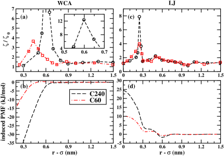
Figure 3: The spatial friction coefficient (panel a) and solvent-induced potential of mean force (panel b) as two C60 (red curve) and two C240 (black curve) approach each other when the solute-solvent interactions are purely repulsive. As expected, there is a greater driving force for assembly with increasing solute length-scale. Panels (c) and (d) depict, respectively, the spatial friction and solvent-induced potential of mean force as two C60 (red curve) and two C240 (black curve) approach each other when the solute-solvent interactions include attraction. In this case, no drying is observed and there is a barrier for desolvation of two water layers as the two bodies approach each other. The friction coefficient is not given at the point of contact for the WCA spheres due to the substantial uncertainty in the correlations of the force fluctuations when the mean force is large.

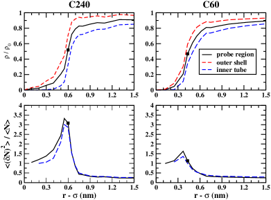
Figure 4: The relative density of water (top row) and the ratio of the variance to the average of the number of water molecules (bottom row) in the probe volume is plotted for C240 (right column) and C60 (left column) when the solute-solvent interaction is purely repulsive. The probe region is divided into an outer shell (red dashed line) and an inter-tube (blue dashed line). The squares indicate the separation at which the friction coefficient is maximum.

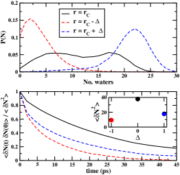
Figure 5: (Top panel) The distribution of number of water molecules present in the probe volume at the critical distance for drying, $r_{c}-\sigma=0.6$ nm (black curve) and at $r=r_{c}\pm\Delta$ where $\Delta=0.1$ nm (red and blue dashed lines). (Bottom panel) At the critical distance there is a slow relaxation observed in the autocorrelation function of the number of molecules in the probe volume as compared to states that are primarily dry or wet. The inset depicts the variance of the number of waters in the probe volume as a function of $\Delta$. All data in this figure pertains to the C240 system when solute-solvent interactions are purely repulsive.

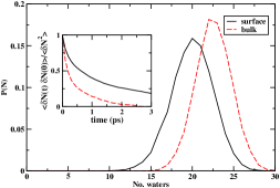
Figure 6: The distribution of water molecules in a probe volume of length $r_{c}-\sigma$ near the surface of a single C240 molecule (solid black curve) and in the bulk (dashed red curve) when the solute-solvent potential is purely repulsive. The inset depicts the autocorrelation function of the number of waters in the probe volume in the respective environments.

V.2 Attractive solute-solvent interactions

Given the high density of carbon sites and the value of $\epsilon_{\text{SS}}$ chosen for the Lennard-Jones potential, the solutes possess a sizable affinity for water when attractive interactions are included. The solvent density is plotted in Fig. 7. The curvature of the surface has a significant impact on water density and fluctuations. For small separations where solvent in the inter-solute region can experience attraction from two bodies, the density is enhanced in areas in the outer probe region where steric repulsion does not dominate. High densities are accompanied by large fluctuations of the number of water molecules in the outer shell. Due to surface curvature, water is first squeezed out from the inner probe volume as the density decreases in this region as the second layer is vacated, and subsequently, the density falls to zero as the final layer of water is removed. In analyzing the trends in the friction coefficient and potential of mean force, the inner probe volume is more indicative of solvent layering.

The induced potential of mean force depicted in the panel (d) of Fig. 3 exhibits minima at separations where one and two water layers are stable at the narrowest portions of the inter-solute region, as indicated by monitoring the inner probe volume. As the spheres come into contact there is a maximum in the solvent induced PMF. Prior calculations of the PMF for a pair of C60 molecules are in qualitative agreement. Makowski et al. (2009) Prior computations of the PMF as two graphene plates approach exhibit barriers for the removal of each solvent layer, Zangi (2011) although the curvature of the spheres gives rise to different behavior than plates at small separations. Namely, as the spheres are curved, the inter-solute region never fully desolvates and the induced mean force opposes assembly until the point of contact.

Upon examination of the spatial dependence of the friction coefficient (panel (c) of Fig. 3), evidence of layering is exhibited by the non-monotonic behavior of the friction coefficient for small separations $r-\sigma<0.5$ nm. The friction coefficient peaks as the PMF rises and the second layer of solvent is removed. At smaller separations, the friction coefficient falls at the minimum of both the induced PMF and solvent fluctuations ($r-\sigma=0.3$ nm), and then as the final water layer vacates the inter-solute region both the PMF and friction coefficient rise sharply, with the size of the latter abating rapidly as solvent density in the inner region decreases. These trends are also witnessed in the water statistics. The point at which the friction coefficient is maximum corresponds to a point where the density is near a maximum, and the fluctuations are large and increasing. The values of the density and fluctuation at the separation of maximum friction coefficient are marked on the curves presented in Fig. 7. In the case of C240, these trends are more clearly observed upon study of the smaller probe volume. It stands to reason that in the case of attractive spheres, the friction exhibits some direct relation to both the density and fluctuations of solvent in the inter-solute region.

The spatial dependence of the friction coefficient is in stark contrast to the predictions of continuum hydrodynamics in the short-range limit, where the friction coefficient is predicted to monotonically increase and diverge as the bodies are brought into contact. This discrepancy is engendered by the layering and granularity of liquids over small length scales. The increase in friction coefficient may have its molecular origins in the confined rattling in the inter-solute region as the water is squeezed out, Bocquet et al. (1997) as is indicated by the large fluctuations in the probe volume (Fig. 7). It is also observed that the spatial friction coefficient plotted in panel (c) of Fig. 3 scales with particle size, that is the curves for C60 and C240 nearly superimpose upon each other when the difference in effective molecular radius is taken into account.

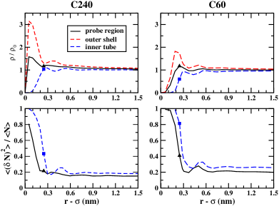
Figure 7: The relative density of water (top row) and the ratio of the variance to the average of the number of water molecules (bottom row) in the probe volume is plotted for C240 (left column) and C60 (right column) when the solute-solvent interaction includes attraction. The probe region is divided into an outer shell (red dashed line) and an inner-tube (blue dashed line). Triangles and squares denote the separation at which the friction coefficient is maximum.

V.3 Diffusion controlled rate

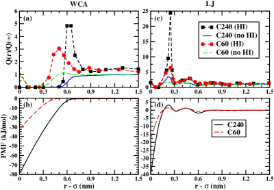
Figure 8: The ratio of the friction coefficient to pair-correlation function, $Q(r)$ is plotted with and without the inclusion of hydrodynamic interactions (HI) as two C240 (black curves that are dotted with squares and dashed, respectively) and two C60 (red curves that are dotted with circles and dashed, respectively) molecules approach when the solute-solvent interactions include attraction (panel a) and for the case when the solute-solvent interaction are purely repulsive (panel c). $Q(\infty)=\zeta_{0}$ is defined as the value of $Q$ for large separations when the potential of mean force and hydrodynamic interactions are negligible. The potential of mean force including the direct interactions between a pair of C240 and C60 molecules with solute-solvent interactions that are purely repulsive (panel b) and include attraction (panel d) is also depicted.

In the high friction limit, a radial Smoluchowski equation describes the motion along the relative coordinate, $r$. The diffusion-controlled rate of reaction can be computed from the following expression Emeis and Fehder (1970); Deutch and Felderhof (1973); Wolynes and Deutch (1976); Northrup and Hynes (1979); Calef and Deutch (1983); Straub et al. (1990):

$$k^{-1}=\frac{1}{4\pi k_{b}T}\int\limits_{\sigma}^{\infty}\mathrm{d}r\;\frac{Q(r)}{r^{2}}$$ (7)

where $\sigma$ is the contact diameter of the Brownian bodies and,

$$Q(r)=\frac{\zeta(r)}{g(r)}\;,$$ (8)

is the ratio of the friction coefficient to the pair-correlation function $g(r)=e^{-\mathcal{W}(r)/k_{b}T}$, where $\mathcal{W}(r)$ is the total potential of mean force that includes contributions from both direct and (induced) solvent-mediated interactions. The full PMF is plotted in panels (b) and (d) of Fig. 8 and for C60 is in good agreement with prior work. Makowski et al. (2009) The function Q(r) is plotted in panels (a) and (c) of Fig. 8 for all combinations of fullerene sizes and interaction potentials presently considered. It is compared with its value if hydrodynamic interactions are neglected, that is when $\zeta(r)=\zeta_{0}$, where $\zeta_{0}$ is one half the friction coefficient on the single body under periodic conditions (see Sec. IV).

In the case of purely repulsive solute-solvent interaction, Q(r) has a markedly different form that depends on whether or not hydrodynamic interactions are included. In particular, due to the fact that the PMF is virtually barrierless when solute-solvent interactions are purely repulsive, hydrodynamic interactions give rise to a maximum in Q(r), as exhibited in panel (a) of Fig. 8. In the case of bodies that attract solvent, Q(r) is also larger when hydrodynamic interactions are included. However in contrast to ideal hydrophobes, the inclusion of spatially dependent friction coefficient tends to “reinforce” the extrema engendered by the PMF. Consistent with the frictional profiles presented in Fig. 3, the impact of hydrodynamic interactions is greatest at separations where drying or desolvation occurs. The function $Q(r)$ is found to increase at small separations, $r-\sigma<0.1\;\text{nm}$, as direct repulsive interactions dominate in this region.

In order to evaluate Eqn. 7, the spatial friction coefficient is approximated for large separations via a switching function Morrone et al. (2010) that smoothly reduces its value to a plateau of $\zeta_{0}$ at a distance $0.5$ nm further than the farthest separation for which the friction coefficient was computed. Although the computed rate constant exhibits weak dependence on the choice of cutoff, this does not alter the observed trends. We note that $\zeta_{0}$ depends on the periodic boundary conditions adopted (see Sec. IV), and, moreover, due to the small relative separations studied in our work, our calculations do not capture the long-range decay of the hydrodynamic interactions. Thus the rate constant for association presently computed accurately reflects the short-range hydrodynamic interaction at the molecular scale but not the contribution of the long range hydrodynamic interactions.

If both the potential of mean force and hydrodynamic interactions are neglected the diffusion controlled rate constant reduces to the familiar expression,

$$k_{0} =\frac{4\pi k_{b}T\sigma}{\zeta_{0}}\;.$$ (9)

The ratio of the rates to $k_{0}$ computed by means of Eqn. 7 with and without the inclusion of hydrodynamic interactions or the potential of mean force are given in Table 2. The values of $k_{0}$ are nearly independent of molecular diameter, which is a consequence of the Stokes-Einstein relation and the direct proportionality of friction coefficient to solute diameter. It can be seen that if the potential of mean force is considered and hydrodynamic interactions are not included (that is $\zeta(r)=\zeta_{0}$), then the rate of “ideal” hydrophobic assembly (when the solute only excludes volume) is increased. In the case of the attractive solutes, there are barriers to assembly and an attractive basin at short range that serve to only modestly impact the rate. The inclusion of hydrodynamic interactions reduces the diffusion controlled rate by approximately $30-40\%$ from its respective value across all systems presently considered. If the potential of mean force (both direct and solvent-induced) is not included in the computation of the rate constant, then one can clearly see that hydrodynamic interactions reduce the rate of association almost uniformly across the four systems studied, this despite the different physics in their separate behaviors (see Fig. 8). This is probably due to the fact that the main quantitative impact of molecular-scale hydrodynamics is to increase the value of $Q(r)$ at separations slightly larger than required for desolvation of the inter-solute region.

Continuum hydrodynamic theory has been utilized to compute the rate of assembly of two bodies. Deutch and Felderhof (1973); Wolynes and Deutch (1976); Sun and Weinstein (2007); Frembgen-Kesner and Elcock (2010) As is well known, the strong divergence of the friction coefficient exhibited by the short-range lubrication expression utilized in Stokesian dynamics and plotted in Fig. 2 prohibits contact and thus the computed rate constant from Eqn. 7 would be zero. Jeffrey and Onishi (1984); Brady et al. (1988); Brady (1988) The lubrication limit for the case of slip boundary conditions as derived by Wolynes and Deutch Wolynes and Deutch (1976) is integrable and hydrodynamic interactions were found to decrease the rate constant by $\approx 30\%$. Recently, hydrodynamics were included by means of the Rotne-Prager tensor in the evaluation of protein-protein association rates and found to decrease the rate of association by $\approx 35-80\%$. Frembgen-Kesner and Elcock (2010) Although these results generally appear in agreement with our work, as noted above, the present estimates only adequately gauge the impact of short-range hydrodynamic interactions and therefore do not readily lend themselves to detailed comparisons.

As stated above, if the spatial dependence of the friction coefficient is neglected, the rate constant for reaction is larger than $k_{0}$ for ideal hydrophobes, as the solvent induced potential of mean force is attractive. This rate constant is reduced by hydrodynamic interactions which, in some sense, capture the timescale associated with dewetting fluctuations (see Sec. V.1). As drying fluctuations are relatively slow (see Fig. 5) this raises the question of whether or not the separation of timescales within the Brownian limit is good description of systems near a drying transition.

		$k/k_{0}$ (HI)	$k/k_{0}$ (No HI)	$k/k_{0}$ (No PMF)	$k_{0}$ ( $10^{10}$ M-1 s-1 )
C60	LJ	0.66	1.02	0.68	1.16
C240	LJ	0.60	0.95	0.74	1.10
C60	WCA	0.93	1.27	0.72	1.54
C240	WCA	0.99	1.37	0.64	1.51

Table 2: Table of the ratio of the diffusion controlled rate constants with and without the inclusion of hydrodynamic interactions or the potential of mean force to the quantity $k_{0}=4\pi k_{b}T\sigma/\zeta_{0}$

VI Discussion and conclusions

The spatial dependence of the friction coefficient in the Brownian limit has been computed as two non-polar bodies come into contact. The system is analyzed within the framework of Brownian dynamics and hydrodynamic interactions are included via explicit molecular dynamics simulation. We find the friction coefficient deviates from continuum hydrodynamic predictions at small separations and dramatically depends on the nature of solute-solvent interactions. For purely repulsive spheres, we find that the friction coefficient peaks at the critical distance for dewetting and decreases as the inter-solute region dries. For attractive solutes water is expelled by steric repulsion and the effects of solvent layering are apparent in the non-monotonic dependence of the friction coefficient on separation. The variation of friction coefficient with separation is due solvent occupation and fluctuations in the inter-solute region. Large solvent fluctuations and slow relaxation times are associated with increasing friction coefficient, and in this way both static and dynamical solvent-mediated effects contribute to the frictional force. Under certain circumstance slow solvent fluctuations in the near drying regime may give rise to non-Markovian effects.

In their study of hydrophobic assembly, Willard and Chandler found that not only the relative separation, but also solvent degrees of freedom, namely the occupancy of the inter-solute region, are necessary to characterize the process. Willard and Chandler (2008) Such behavior has also been observed in the assembly of hydrophobic plates. Huang et al. (2003, 2005) As our analysis is in the framework of Brownian dynamics, only solute degrees of freedom are explicitly treated in the rate calculation presented in Sec. V.3. However, solvent fluctuations engender the peak in the spatially dependent friction coefficient observed at the dewetting transition. In this way, drying phenomena manifests itself when molecular-scale hydrodynamic interactions are included in the Brownian limit.

The Brownian description is valid if the motion of the solute occurs on a much slower time scale than the solvent dynamics. We find that relatively slow solvent motions are present at the critical separation for dewetting, which raises questions about the validity of the Markovian assumption. We found the correlation time for water fluctuations in the inter-solute region at the critical separation to be $\approx 25$ ps for C240. (see Fig. 5). Prior work has shown that the timescale for hydrophobic assembly depends on not only the size of the solutes but also on the nature of the interactions, Huang et al. (2003, 2005) and the time scale for solvent fluctuations can be much longer than 25 ps. In the case where solvent fluctuations cannot be considered fast with respect to solute diffusion, one may consider alternative formulations that include dynamical disorder Zwanzig (1990), and the use of techniques for extracting the spatially dependent memory kernel within the framework of the generalized Langevin equation. Berne and Harp (1970); Straub et al. (1987, 1990) Naturally, the time scales will depend upon the size of the solute, and future studies may be designed to more fully probe this observation.

Recently, hydrodynamic interactions have been shown to significantly decrease in vivo diffusion in cellular environments. Ando and Skolnick (2010) As the present computation is limited to two bodies in a solvent bath, one can only draw limited parallels to behavior in crowded systems. With this caveat in mind, we find some correspondence in our study where we find that inclusion of hydrodynamic interactions leads to a decrease of the diffusion controlled rate constant for assembly by approximately $30-40\%$. For barrierless “ideal” hydrophobic assembly along the relative coordinate, hydrodynamic interactions introduce a frictional “barrier” that retards the rate of assembly (see Fig. 8), whereas in the case of attractive solvents the main effect is to enhance the maxima engendered by the potential of mean force. In this way, the interplay between hydrodynamic interactions and the free energy surface strongly depends on solvent-solute coupling. Future work will be aimed at exploring these insights and applying them to study diffusive phenomena in nanoscopic systems.

Appendix A Calculation of the spatially dependent friction coefficient

A.1 Two-body friction tensor

In this work, we study the spatially dependent friction coefficient along the relative distance between two bodies, $r=\left|\vec{r}_{2}-\vec{r}_{1}\right|$. The complete friction coefficient tensor is related to the motion of all $3N$ degrees of freedom. The tensor relates the frictional force to the particle velocities. For $N=2$ this can be expressed as,

$$\left(\begin{array}[]{c}\delta\vec{F}_{1}\\ \delta\vec{F}_{2}\end{array}\right) =\left(\begin{array}[]{cc}\mathrm{\underline{\underline{\zeta}}}_{11}(r)&\mathrm{\underline{\underline{\zeta}}}_{12}(r)\\ \mathrm{\underline{\underline{\zeta}}}_{21}(r)&\mathrm{\underline{\underline{\zeta}}}_{22}(r)\end{array}\right)\left(\begin{array}[]{c}\vec{v}_{1}\\ \vec{v}_{2}\end{array}\right)\;,$$ (16)

where $\delta\vec{F}$ is the deviation of the force on the sphere from its mean value. The friction coefficient tensor $\mathrm{\underline{\underline{\zeta}}}(r)$ has dimension of $6\times 6$ and may be decomposed into four blocks that correspond to self and cross interactions between the bodies. Each submatrix is a diagonal $3\times 3$ matrix,

$$\mathrm{\underline{\underline{\zeta}}}=\left(\begin{array}[]{ccc}\zeta_{\|}&0&0\\ 0&\zeta_{\bot}&0\\ 0&0&\zeta_{\bot}\end{array}\right),$$ (20)

if the coordinate system is defined such that one direction is parallel and two directions are perpendicular to the line of centers. The two spheres are identical so by symmetry $\mathrm{\underline{\underline{\zeta}}}_{11}(r)=\mathrm{\underline{\underline{\zeta}}}_{22}(r)$ and $\mathrm{\underline{\underline{\zeta}}}_{12}(r)=\mathrm{\underline{\underline{\zeta}}}_{21}(r)$. The friction coefficient along the relative coordinate, $r=r_{2,\|}-r_{1,\|}$, may be obtained from manipulation of Eqn. 16. The following relation can then be extracted,

$$\zeta_{\text{rel}}(r)=\frac{1}{2}\left(\zeta_{11,\|}(r)-\zeta_{12,\|}(r)\right)\;,$$ (21)

and associated to the Langevin equation given by Eqn. 1.

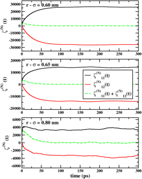
Figure 9: The time integral of the self (black curve) and cross (red curve) force-force autocorrelation functions and the sum of these two functions (green curve) is plotted as two C240 molecules approach each other and interact with the solvent purely by means of repulsion. The top panel, center, and bottom panel depict this quantity at different separations. One can see that the self and cross autocorrelation functions plateau at a non-zero value, though their sum decays to zero, in agreement with the finding of Bocquet et al. Bocquet et al. (1997) The friction coefficient is plotted in units of (kj/mol) $\cdot$ (ps/nm²).

A.2 Review of techniques relating the friction coefficient to molecular dynamics simulation

Here we review the techniques developed in Refs. Bocquet et al., 1994 and Bocquet et al., 1997 for the extraction of the Brownian friction coefficient from molecular dynamics simulations. First consider a single Brownian sphere of mass, $M$, in a bath of $N$ solvent molecules of mass, $m$. This comprises an isolated system. Next we consider the limit, $M\rightarrow\infty$, in which the solute particles are fixed. In this case, the total solvent momentum is not a conserved quantity. As shown below, the computation of the friction coefficient is essentially a probe of the total momentum relaxation.

We begin by relating the rate of change of the total solvent momentum $P(t)$ to the force acting on the solute $\mathcal{F}(t)$ by means of Newton’s third law.

$$\mathcal{F}(t) =-\dot{P}(t)$$ (22)

To simplify the notation we only consider one dimension, although the expressions for three-dimensions are readily obtainable. Next, consider the integral that in the $t\rightarrow\infty$ and $N\rightarrow\infty$ limit yields the Green Kubo relation for the friction coefficient. This can be expressed in terms of the total solvent momentum:

$$\zeta(t) =\frac{1}{k_{b}T}\int\limits_{0}^{t}\mathrm{d}\tau\left<\mathcal{F}(0)\mathcal{F}(-\tau)\right>$$ (23)

$$=-\frac{1}{k_{b}T}\left<\dot{P}(t)P(0)\right>$$ (24)

Onsager’s principle linearly relates the force acting on the solute to the total solvent momentum in the long time limit:

$$\mathcal{F}(t) =\frac{\zeta}{Nm}P(t)$$ (25)

$$\dot{P}(t) =-\frac{\zeta}{Nm}P(t)$$ (26)

Where Eqn. 26 arises from combining Eqn. 22 and Eqn. 25. Utilizing Eqn. 24, it can readily shown that $\zeta(t)$ has the simple form:

$$\zeta(t) =\zeta e^{-\zeta t/Nm}.$$ (27)

Both the $t\rightarrow\infty$ and $N\rightarrow\infty$ limits must be applied in order calculate the friction coefficient in the linear response regime (See Eqn. 3). If the time limit is taken first, as is necessarily the case when computing the property in a simulation of finite size, then $\zeta(\infty)\rightarrow 0$. However, if the thermodynamic limit is taken first ($N\rightarrow\infty$), then a finite and correct value for the friction coefficient may be recovered. Prior work has shown that instead of directly applying the Green-Kubo relation, the friction coefficient may be recovered by probing the relaxation of $\zeta(t)$. Presently this was achieved by an analysis of the Laplace transform of Eqn. 27 developed in Ref. Bocquet et al., 1994.

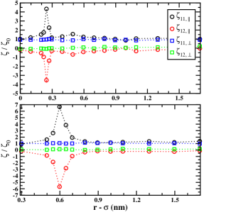
Figure 10: The unique components of the friction coefficient tensor as two C240 molecules approach each other and interact with the solvent with attractive (top panel) or purely repulsively (bottom panel) forces. The self term parallel (black circles) and perpendicular (blue squares) to the line of solute centers is plotted alongside the cross friction coefficient in the parallel (red circles) and perpendicular (green squares) direction.

In the case of the two body friction coefficient we begin by defining the integral of the naive MD estimate for each submatrix of the friction coefficient tensor that one arrives at from the direct application of the Green-Kubo relation:

$$\zeta_{11}^{(N)}(t) =\frac{1}{k_{b}T}\int\limits_{0}^{t}\mathrm{d}\tau\;\left<\delta F_{1}(t)\delta F_{1}(0)\right>$$ (28)

$$\zeta_{12}^{(N)}(t) =\frac{1}{k_{b}T}\int\limits_{0}^{t}\mathrm{d}\tau\;\left<\delta F_{1}(t)\delta F_{2}(0)\right>$$ (29)

The superscript $N$ denotes the number of solvent molecules present in the simulation. When two Brownian bodies are present, the solvent momentum relaxation is related to the sum of the fluctuations of forces on the two spheres, $\dot{P}(t)=-(\delta F_{1}(t)+\delta F_{2}(t))$. Analogous to case of a single body in a bath reviewed above, when the long time limit is taken for finite $N$, it was shown in Ref. Bocquet et al., 1997 that

$$\zeta_{11}^{(N)}(\infty)+\zeta_{12}^{(N)}(\infty) =-\int\limits_{0}^{\infty}\mathrm{d}\tau\left<\dot{P}(t)\delta F_{1}(0)\right>$$

$$=0$$ (30)

This spurious result is due to finite size effects and is demonstrated numerically in Fig. 9. Although the measured force-force correlation functions of Eqn. 28 and Eqn. 29 plateau to non-zero values, their sum does indeed decay to zero. Bocquet et al. proceed to relate the integrals of the force-force autocorrelation functions with their proper $N\rightarrow\infty$ limits. Details are given in Ref. Bocquet et al., 1997. This analysis yields relations of the plateaus of the components of $\mathrm{\underline{\underline{\zeta}}}^{(N)}(t)$ to a linear combination of components of the friction coefficient tensor $\mathrm{\underline{\underline{\zeta}}}$ that correctly approach the thermodynamic limit.

$$\frac{1}{2}\left(\mathrm{\underline{\underline{\zeta}}}_{11}-\mathrm{\underline{\underline{\zeta}}}_{12}\right)=\mathrm{\underline{\underline{\zeta}}}_{11}^{(N)}(\infty)=-\mathrm{\underline{\underline{\zeta}}}_{12}^{(N)}(\infty).$$ (31)

It can be readily seen that the component of the linear combination parallel to axis of centers can be identified with the friction coefficient in the relative directions that is reported in Fig. 3. In order to obtain the full friction coefficient tensor, one more relation must be identified,

$$-\frac{2}{Nmk_{b}T}\left(\mathrm{\underline{\underline{\zeta}}}_{11}+\mathrm{\underline{\underline{\zeta}}}_{12}\right)t =\ln\left(\frac{\mathrm{\underline{\underline{\zeta}}}_{11}^{(N)}(t)+\mathrm{\underline{\underline{\zeta}}}_{12}^{(N)}(t)}{\mathrm{\underline{\underline{\zeta}}}_{11}^{(N)}(0)+\mathrm{\underline{\underline{\zeta}}}_{12}^{(N)}(0)}\right)\;,$$ (32)

which characterizes the relaxation of the sum of the force-force correlation functions plotted in Fig. 9 to zero. The resulting friction coefficient tensor for the C240 fullerene model with purely repulsive and attractive solute-solvent interactions is plotted in Fig. 10. It can be seen that the friction coefficient is primarily perturbed in the direction of the relative coordinate, and the perpendicular components of the self sub-matrix ($\zeta_{11,\|}$) have limited spatial dependence and their values are closer to the single body result. Concurrently, the value of $\zeta_{12,\bot}$ remains near zero.

There is less than a 10% error in the estimation of the friction coefficient provided by Ref. Bocquet et al., 1997. Estimates of error have been obtained from the variance of the measured plateau or from the difference between elements of the full friction coefficient tensor that are equivalent by symmetry.

References

- Pangali et al. (1979) C. Pangali, M. Rao, and B. J. Berne, J. Chem. Phys. 71, 2982 (1979).
- Chandler (2005) D. Chandler, Nature 437, 640 (2005).
- Berne et al. (2009) B. J. Berne, J. D. Weeks, and R. Zhou, Annu. Rev. Phys. Chem. 60, 85 (2009).
- Jamadagni et al. (2011) S. N. Jamadagni, R. Godawat, and S. Garde, Annu. Rev. Chem. and Biomol. Eng. 2, 147 (2011).
- Wallqvist and Berne (1995) A. Wallqvist and B. J. Berne, J. Phys. Chem. 99, 2893 (1995).
- Hummer et al. (1996) G. Hummer, S. Garde, A. E. García, A. Pohorille, and L. R. Pratt, Proc. Natl. Acad. Sci. 93, 8951 (1996).
- Lum et al. (1999) K. Lum, D. Chandler, and J. Weeks, J. Phys. Chem. B 103, 4570 (1999).
- Huang and Chandler (2002) D. M. Huang and D. Chandler, J. Phys. Chem. B 106, 2047 (2002).
- Ten Wolde and Chandler (2002) P. R. Ten Wolde and D. Chandler, Proc. Natl. Acad. Sci. 99, 6539 (2002).
- Huang et al. (2003) X. Huang, C. J. Margulis, and B. J. Berne, Proc. Natl. Acad. Sci. 100, 11953 (2003).
- Zhou et al. (2004) R. Zhou, X. Huang, C. J. Margulis, and B. J. Berne, Science 305, 1605 (2004).
- Huang et al. (2005) X. Huang, R. Zhou, and B. J. Berne, J. Phys. Chem. B 109, 3546 (2005).
- Giovambattista et al. (2007) N. Giovambattista, P. G. Debenedetti, and P. J. Rossky, J. Phys. Chem. B 111, 9581 (2007).
- Mittal and Hummer (2008) J. Mittal and G. Hummer, Proc. Natl. Acad. Sci. 105, 20130 (2008).
- Willard and Chandler (2008) A. P. Willard and D. Chandler, J. Phys. Chem. B 112, 6187 (2008).
- Sarupria and Garde (2009) S. Sarupria and S. Garde, Phys. Rev. Lett. 103, 037803 (2009).
- Godawat et al. (2009) R. Godawat, S. N. Jamadagni, and S. Garde, Proc. Natl. Acad. Sci. 106, 15119 (2009).
- Patel et al. (2010) A. J. Patel, P. Varilly, and D. Chandler, J. Phys. Chem. B 114, 1632 (2010).
- Huang et al. (2008) D. M. Huang, C. Sendner, D. Horinek, R. R. Netz, and L. Bocquet, Phys. Rev. Lett. 101, 226101 (2008).
- Sendner et al. (2009) C. Sendner, D. Horinek, L. Bocquet, and R. R. Netz, Langmuir 25, 10768 (2009).
- Thomas and McGaughey (2009) J. A. Thomas and A. J. H. McGaughey, Phys. Rev. Lett. 102, 184502 (2009).
- Kalra et al. (2010) A. Kalra, S. Garde, and G. Hummer, Euro. Phys. J. Special Topics 189, 147 (2010).
- Falk et al. (2010) K. Falk, F. Sedlmeier, L. Joly, R. R. Netz, and L. Bocquet, Nano Lett. 10, 4067 (2010).
- Bocquet and Charlaix (2010) L. Bocquet and E. Charlaix, Chem. Soc. Rev. 39, 1073 (2010).
- Ermak and McCammon (1978) D. L. Ermak and J. A. McCammon, J. Chem. Phys. 69, 1352 (1978).
- Brady et al. (1988) J. F. Brady, R. J. Philips, J. C. Lester, and G. Bossis, J. Fluid Mech. 195, 257 (1988).
- Brady (1988) J. Brady, Annu. Rev. Fluid Mech 20, 111 (1988).
- Chatterji and Horbach (2005) A. Chatterji and J. Horbach, J. Chem. Phys. 122, 184903 (2005).
- Padding and Louis (2006) J. T. Padding and A. A. Louis, Phys. Rev. E 74, 031402 (2006).
- Ando and Skolnick (2010) T. Ando and J. Skolnick, Proc. Natl. Acad. Sci. 107, 18457 (2010).
- Berne and Harp (1970) B. J. Berne and G. D. Harp, Adv. Chem . Phys. 17, 1 (1970).
- Straub et al. (1987) J. E. Straub, M. Borkovec, and B. J. Berne, J. Phys. Chem. 91, 4995 (1987).
- Straub et al. (1990) J. E. Straub, B. J. Berne, and B. Roux, J. Chem. Phys. 93, 6804 (1990).
- Español and Zúñiga (1993) P. Español and I. Zúñiga, J. Chem. Phys. 98, 574 (1993).
- Bocquet et al. (1994) L. Bocquet, J. Hansen, and J. Piasecki, J. Stat. Phys. 76, 527 (1994).
- Bocquet et al. (1997) L. Bocquet, J. Hansen, and J. Piasecki, J. Stat. Phys. 89, 321 (1997).
- Lee (2010) S. H. Lee, Bull. Korean Chem. Soc. 31, 2402 (2010).
- Bezmel’nitsyn et al. (1998) V. N. Bezmel’nitsyn, A. V. Eletskii, and M. V. Okun, Physics - Uspekhi 41, 1091 (1998).
- Hotta et al. (2005) T. Hotta, A. Kimura, and M. Sasai, J. Phys. Chem. B 109, 18600 (2005).
- Makowski et al. (2009) M. Makowski, C. Czaplewski, A. Liwo, and H. A. Scheraga, J. Phys. Chem. B 114, 993 (2009).
- Emeis and Fehder (1970) C. A. Emeis and P. L. Fehder, J. Am. Chem. Soc. 92, 2246 (1970).
- Deutch and Felderhof (1973) J. M. Deutch and B. U. Felderhof, J. Chem. Phys. 59, 1669 (1973).
- Wolynes and Deutch (1976) P. G. Wolynes and J. M. Deutch, J. Chem. Phys. 65, 450 (1976).
- Northrup and Hynes (1979) S. H. Northrup and J. T. Hynes, J. Chem. Phys. 71, 871 (1979).
- Calef and Deutch (1983) D. F. Calef and J. M. Deutch, Annu. Rev. Phys. Chem. 34, 493 (1983).
- Dhont (1996) J. K. G. Dhont, An Introduction to Dynamics of Colloids, edited by D. Mobius and R. Miller, Studies in Interface Science, Vol. 2 (Elsevier, Amsterdam, 1996).
- Jeffrey and Onishi (1984) D. J. Jeffrey and Y. Onishi, J. Fluid Mech. 139, 261 (1984).
- Beenakker (1986) C. Beenakker, J. Chem. Phys. 85, 1581 (1986).
- Chen (1998) S. Chen, Annu. Rev. Fluid Mech. 30, 329 (1998).
- Nakayama et al. (2008) Y. Nakayama, K. Kim, and R. Yamamoto, Euro. Phys. J. E 26, 361 (2008).
- Voulgarakis and Chu (2009) N. K. Voulgarakis and J. Chu, J. Chem. Phys. 130, 134111 (2009).
- Hasimoto (1959) H. Hasimoto, J. Fluid Mech. 5, 317 (1959).
- Lindbo and Tornberg (2010) D. Lindbo and A. K. Tornberg, J. Comput. Phys. 229, 8994 (2010).
- Berne and Pecora (1990) B. J. Berne and R. Pecora, Dynamic Light Scattering: with applications to Chemistry, Biology and Physics (Dover, 1990).
- Weeks et al. (1971) J. D. Weeks, D. Chandler, and H. C. Andersen, J. Chem. Phys. 54, 5237 (1971).
- Jorgensen and Madura (1985) W. L. Jorgensen and J. D. Madura, J. Chem. Phys. 56, 1381 (1985).
- Humphrey et al. (1996) W. Humphrey, A. Dalke, and K. Schulten, J. Molec. Graphics 14, 33 (1996).
- Berendsen et al. (1984) H. J. C. Berendsen, J. P. M. Postma, W. F. van Gunsteren, A. DiNola, and J. R. Haak, J. Chem. Phys. 81, 3684 (1984).
- Bussi et al. (2007) G. Bussi, D. Donadio, and M. Parrinello, J. Chem. Phys. 126, 014101 (2007).
- Hess et al. (2008) B. Hess, C. Kutzner, and D. van der Spoel, J. Chem. Theor. Comput. 4, 435 (2008).
- Weiss et al. (2008) D. R. Weiss, T. M. Raschke, and M. Levitt, J. Phys. Chem. B 112, 2981 (2008).
- Yeh and Hummer (2004) I. C. Yeh and G. Hummer, J. Phys. Chem. B 108, 15873 (2004).
- Gonzalez and Abascale (2010) M. A. Gonzalez and J. F. Abascale, J. Chem. Phys. 132, 096101 (2010).
- Schmidt and Skinner (2003) J. R. Schmidt and J. L. Skinner, J. Chem. Phys. 119, 8062 (2003).
- Schmidt and Skinner (2004) J. R. Schmidt and J. L. Skinner, J. Phys. Chem. B 108, 6767 (2004).
- Li (2009) Z. Li, Phys. Rev. E 80, 061204 (2009).
- Zangi (2011) R. Zangi, J. Phys. Chem. B 115, 2303 (2011).
- Morrone et al. (2010) J. A. Morrone, R. Zhou, and B. J. Berne, J. Chem. Theor. Comput. 6, 1798 (2010).
- Sun and Weinstein (2007) J. Sun and H. Weinstein, J. Chem. Phys. 127, 155105 (2007).
- Frembgen-Kesner and Elcock (2010) T. Frembgen-Kesner and A. H. Elcock, Biophys. J. 99, L75 (2010).
- Zwanzig (1990) R. Zwanzig, Acc. Chem. Res. 23, 148 (1990).