Engineering Benchmarks for Planning: the Domains Used in the Deterministic Part of IPC-4

Abstract

In a field of research about general reasoning mechanisms, it is essential to have appropriate benchmarks. Ideally, the benchmarks should reflect possible applications of the developed technology. In AI Planning, researchers more and more tend to draw their testing examples from the benchmark collections used in the International Planning Competition (IPC). In the organization of (the deterministic part of) the fourth IPC, IPC-4, the authors therefore invested significant effort to create a useful set of benchmarks. They come from five different (potential) real-world applications of planning: airport ground traffic control, oil derivative transportation in pipeline networks, model-checking safety properties, power supply restoration, and UMTS call setup. Adapting and preparing such an application for use as a benchmark in the IPC involves, at the time, inevitable (often drastic) simplifications, as well as careful choice between, and engineering of, domain encodings. For the first time in the IPC, we used compilations to formulate complex domain features in simple languages such as STRIPS, rather than just dropping the more interesting problem constraints in the simpler language subsets. The article explains and discusses the five application domains and their adaptation to form the PDDL test suites used in IPC-4. We summarize known theoretical results on structural properties of the domains, regarding their computational complexity and provable properties of their topology under the $h^{+}$ function (an idealized version of the relaxed plan heuristic). We present new (empirical) results illuminating properties such as the quality of the most wide-spread heuristic functions (planning graph, serial planning graph, and relaxed plan), the growth of propositional representations over instance size, and the number of actions available to achieve each fact; we discuss these data in conjunction with the best results achieved by the different kinds of planners participating in IPC-4.

1 Introduction

Today, to a large extent the research discipline of AI planning is concerned with improving the performance of domain independent generative planning systems. A domain independent generative planning system (planner) must be able to fully automatically find plans: solution sequences in declaratively specified transition systems. The simplest planning formalism is deterministic planning. There, a planner is given as input a set of state variables (often just Booleans, called facts), an initial state (a value assignment to the variables), a goal (a formula), and a set of actions (with a precondition formula describing applicability, and with an effect specifying how the action changes the state). A plan is a time-stamped sequence of actions that maps the initial state into a state that satisfies the goal. This sort of formalism is called deterministic since the initial state is fully specified and the effects of the actions are non-ambiguous. Both restrictions may be weakened to obtain non-deterministic and probabilistic planning.

Performance of planners is measured by testing them on benchmark example instances of the planning problem. The “best” algorithm at any point in time is, generally, considered to be the one that solves these examples most efficiently. In particular, this is the idea in the International Planning Competition (IPC), a biennial event aimed at showcasing the capabilities of current planning systems.

The first IPC took place in 1998, so at the time of writing there were four such events. Providing details about the IPC is beyond the scope of this paper, and we refer the reader to the overview articles written by the organizers of the respective IPC editions (?, ?, ?, ?). In particular, ? (?) provide details about the 4th IPC, such as overall organization, different tracks, evaluation, participating planners, and results. Basic information is included in this paper, so the reader should be able to follow the main discussion without a detailed background. The language used to describe planning problems in the IPC is called PDDL: Planning Domain Definition Language. It was introduced by ? (?) for the first IPC, IPC-1, in 1998. A subset of the language was selected by ? (?) for IPC-2 in 2000. The language was extended with temporal and numerical constructs by ? (?) to form the language PDDL2.1 for IPC-3 in 2002. It was further extended with two additional constructs, “timed initial literals” and “derived predicates”, by ? (?) to form the language PDDL2.2 for IPC-4 in 2004.

Since, even in its simplest forms, AI planning is a computationally hard problem, no system can work efficiently in all problem instances (?, ?). Thus, it is of crucial importance what kinds of examples are used for testing. Today, more and more, AI Planning researchers draw their testing examples from the collections used in the IPC. This makes the IPC benchmarks a very important instrument for the field. In the organization of the deterministic part of the 4th IPC (there was also a probabilistic part, see ?), the authors therefore invested considerable effort into creating a set of “useful” benchmarks for planning.

The very first question to answer is what precisely is meant here by the word “useful”. This is not an easy question. There is no widely accepted mathematical definition for deciding whether a set of benchmarks should be considered useful. There are, however, widely accepted intuitions of when this is the case. Benchmarks should be:

1. Oriented at applications – a benchmark should reflect an application of the technology developed in the field.

2. Diverse in structure – a set of benchmarks should cover different kinds of structure, rather than re-state very similar tasks.

The first of these is usually considered particularly important – indeed, AI planning has frequently been criticized for its “obsession with toy examples”. In recent years, the performance of state-of-the-art systems has improved dramatically, and with that more realistic examples have come within reach. We made another step in this direction by orienting most of the IPC-4 benchmarks at application domains. While traditionally planning benchmarks were more or less fantasy products created having some “real” scenario in mind, we took actual (possible) applications of planning technology, and turned them into something suitable for the competition. We considered five different application domains: airport ground traffic control (Airport), oil derivative transportation in pipeline networks (Pipesworld), model checking safety properties (Promela), power supply restoration (PSR), and setup of mobile communication in UMTS (UMTS). Of course, in the adaptation of an application for use in the IPC, simplifications need to be made. We will get back to this below.

Diverse structure of benchmarks has traditionally been given less attention than realism, but we believe that it is no less important. The structure underlying a testing example determines the performance of the applied solving mechanism. This is particularly true for solving mechanisms whose performance rises and falls with the quality of a heuristic they use. Hoffmann’s (?, ?, ?) results suggest that much of the spectacular performance of modern heuristic search planners is due to structural similarities between most of the traditional planning benchmarks. While this does not imply that modern heuristic search planners aren’t useful, it certainly shows that in the creation of benchmarks there is a risk of introducing a bias towards one specific way of solving them. In selecting the benchmark domains for IPC-4, we tried to cover a range of intuitively very different kinds of problem structure. We will get back to this below.

On the one hand, a creator of planning benchmarks has the noble goal of realistic, and structurally diverse, benchmark domains. On the other hand, he/she has the more pragmatic goal to come up with a version/representation of the benchmarks that can be attacked with existing planning systems. Given the still quite restricted capabilities of systems, obviously the two goals are in conflict. To make matters worse, there isn’t an arbitrarily large supply of planning applications that are publicly available, and/or whose developers agree to have their application used as the basis of a benchmark. For the IPC organizer, on top of all this, the final benchmarks must be accessible for a large enough number of competing systems, which means they must be formulated in a language understood by those systems. Further, the benchmarks must show differences between the scalability of planners, i.e., they must not be too easy or too hard, thus straddling the boundary of current system capabilities.

The solution to the above difficulties, at least our solution in the organization of IPC-4, involved a slow tedious interleaved process of contacting application developers, choosing domains, exploring domain versions, and engineering domain version representations. This article presents, motivates, and discusses our choice of benchmark domains for IPC-4; it explains the engineering processes that led to the finally used domain versions and instances. Further, we report about, and present some new data determining certain structural properties of the resulting benchmarks (more details below). The main contribution of the work is the set of benchmarks, provided in IPC-4. The contributions of this article are: first, providing the necessary documentation of these benchmarks; second, describing the technical processes used in their creation; third, providing an extensive discussion of the structural properties of the benchmarks. Apart from these more technical contributions, we believe that our work has value as an example of a large-scale attempt at engineering a useful set of benchmarks for classical planning.

It is difficult to make any formal claim about our created set of benchmarks, such as that they are in some way better than the previous benchmarks. When working on this, our intent was to overcome certain shortcomings of many benchmarks, though one would be hard pressed to come up with a formal proof that such improvements were indeed made. After all, judging the quality of a set of benchmarks is a rather complex matter guided mostly by intuitions, and, worse, personal opinions. What we did was, do our best to create as realistic, structurally diverse, and accessible benchmarks as possible for IPC-4. Our belief is that we succeeded in doing so. The benchmarks definitely differ in certain ways from most of the previous benchmarks. We think that most of these differences are advantageous; we will discuss this at the places where we point out the differences.

Regarding realism of the benchmarks, as pointed out above, the main step we took was to design benchmarks “top-down”, i.e., start from actual possible applications of planning technology, and turn them into something suitable for the competition – rather than the more traditional “bottom-up” approach of just artificially creating a domain with some “real” scenario in mind. Of course, for modelling an application in PDDL, particularly for modelling it in a way making it suitable for use in the IPC, simplifications need to be made. In some cases, e.g., airport ground traffic control, the simplifications were not overly drastic, and preserved the overall properties and intuitive structure of the domain. But in other cases, e.g., oil derivative transportation in pipeline networks, the simplifications we needed to make were so drastic that these domains could just as well have been created in the traditional bottom-up way. Still, even if greatly simplified, a domain generated top-down has a better chance to capture some structure relevant in a real application. Moreover, a top-down domain has the advantage that since it is derived from a real application, it provides a clear guideline towards more realism; the future challenge is to make planners work on more realistic encodings of the application. In the previous competitions, the only domains generated top-down in the above sense were the Elevator domain used in IPC-2 (?, ?), and the Satellite and Rovers domains used in IPC-3 (?).

Regarding diverse structure of the benchmarks, in contrast to the previous competitions, in the IPC-4 domains there is no common “theme” underlying many of the benchmarks. In IPC-1, 5 out of 7 domains were variants of transportation; in IPC-2, 4 out of 7 domains were variants of transportation; in IPC-3, 3 out of 6 domains were variants of transportation, and 2 were about gathering data in space. Some of the “variants” are in fact very interesting in their use of constructs such as locked locations, fuel units, road map graphs, stackable objects, and complex side constraints. However, there is certainly an intuitive similarity in the structure and relationships in the domains. To some extent this similarity is even automatically detectable (?). Not so in IPC-4: airport ground traffic control, oil derivative transportation in pipeline networks, model checking safety properties, power supply restoration, and UMTS call setup are rather different topics. At most one could claim that airport ground traffic control and UMTS call setup both have a scheduling nature. We will see, however, that the IPC-4 version of airport ground traffic control allows considerably more freedom than classical scheduling formulations, making it a PSPACE-complete decision problem. The particulars of the domains will be overviewed in Section 3.

Approaching “structure” from a more formal point of view is more difficult. It is largely unclear what, precisely, the relevant structure in a planning domain/instance is, in a general sense. While ? (?, ?, ?) provides one possible definition – search space surface topology under a certain heuristic function – there are many other possible options. In particular, Hoffmann’s results are relevant only for heuristic search planners that generate their heuristic functions based on the “ignoring delete lists” relaxation (?, ?, ?, ?, ?). For lack of a better formal handle, we used Hoffmann’s definitions to qualify the structure of the domains. The selected domains cover different regions of Hoffmann’s “planning domain taxonomy”, in particular they lie in regions that have less coverage in the traditional benchmarks. Because they are interesting in the context of the paper at hand, we summarize Hoffmann’s (?) results for 30 domains including all domains used in the previous competitions. We also summarize Helmert’s (?) results on the computational complexity of satisficing and optimal planning in the IPC-4 domains. It turns out that their complexity covers a wide range – the widest possible range, for propositional planning formalisms – from PSPACE-hard to polynomial. We finally provide some new data to analyze the structural relationships and differences between the domains. Amongst other things, for each instance, we measure: the number of (parallel and sequential) steps needed to achieve the goal, estimated by the smallest plan found by any IPC-4 participant; the same number as estimated by planning graphs and relaxed plans; and the distribution of the number of possible achieving actions for each fact. The results are examined in a comparison between the different domains, taking into account the runtime performance exhibited by the different kinds of planners in IPC-4.

Apart from realism and diverse structure, our main quest in the creation of the IPC-4 benchmarks was to promote their accessibility. Applications are, typically, if they can be modelled at all in PDDL, most naturally modelled using rather complex language constructs such as time, numeric variables, logical formulas, and conditional effects. Most existing systems handle only subsets of this, in fact more than half of the systems entered into IPC-4 (precisely, 11 out of 19) could handle only the simple STRIPS language, or slight extensions of it. In the previous competitions, as done for example in the Elevator, Satellite, and Rovers domains, this was handled simply by dropping the more interesting domain constraints in the simpler languages, i.e., by removing the respective language constructs from the domain/instance descriptions. In contrast, for the first time in the IPC, we compiled as much of the domain semantics as possible down into the simpler language formats. Such a compilation is hard, sometimes impossible, to do. It can be done for ADL constructs, as well as for the two new constructs introduced for the IPC-4 language PDDL2.2, derived predicates and timed initial literals. We implemented, and applied, compilation methods for all these cases. The compilations serve to preserve more of the original domain structure, in the simpler language classes. For example, the STRIPS version of the Elevator domain in IPC-2 is so simplified from the original ADL version that it bears only marginal similarity to real elevator control – in particular, the planner can explicitly tell passengers to get into or out of the lift. In contrast, our STRIPS formulation of the airport ground traffic domain is, semantically, identical to our ADL formulation – it expresses the same things, but in a more awkward fashion.

The compiled domain “versions” were offered to the competitors as alternative domain version “formulations”, yielding a 2-step hierarchy for each domain. That is, each domain in IPC-4 could contain several different domain versions, differing in terms of the number of domain constraints/properties considered. Within each domain version, there could be several domain version formulations, differing in terms of the language used to formulate the (same) semantics. The competitors could choose, within each version, whichever formulation their planners could handle best/handle at all, and the results within the domain version were then evaluated together. This way, we intended to make the competition as accessible as possible while at the same time keeping the number of separation lines in the data – the number of distinctions that need to be made when evaluating the data – at an acceptable level.

We are, of course, aware that encoding details can have a significant impact on system performance. Particularly, when compiling ADL to STRIPS, in most cases we had to revert to fully grounded encodings. While this certainly isn’t desirable, we believe it to be an acceptable price to pay for the benefit of accessibility. Most current systems ground the operators out as a pre-process anyway. In cases where we considered the compiled domain formulations too different from the original ones to allow for a fair comparison – typically because plan length increased significantly due to the compilation – the compiled formulation was posed to the competitors as a separate domain version.

The article is organized as follows. The main body of text contains general information. In Section 2, we give a detailed explanation of the compilation methods we used. In Section 3, we give a summary of the domains, each with a short application description, our motivation for including the domain, a brief explanation of the main simplifications made, and a brief explanation of the different domain versions and formulations. In Section 4, we summarize Hoffmann’s (?) and Helmert’s (?) theoretical results on the structure of the IPC-4 domains. Section 5, we provide our own empirical analysis of structural properties. Section 6 discusses what was achieved, and provides a summary of the main issues left open. For each of the IPC-4 domains, we include a separate section in Appendix A, providing detailed information on the application, its adaptation for IPC-4, its domain versions, the example instances used, and future directions. Although these details are in an appendix, we emphasize that this is not because they are of secondary importance. On the contrary, they describe the main body of work we did. The presentation in an appendix seems more suitable since we expect the reader to, typically, examine the domains in detail in a selective and non-chronological manner.

2 PDDL Compilations

We used three kinds of compilation methods:

• ADL to SIMPLE-ADL (STRIPS with conditional effects) or STRIPS;

• PDDL with derived predicates to PDDL without them;

• PDDL with timed initial literals to PDDL without them.

We consider these compilation methods in this order, explaining, for each, how the compilation works, what the main difficulties and their possible solutions are, and giving an outline of how we used the compilation in the competition. Note that ADL, SIMPLE-ADL, and STRIPS are subsets of PDDL. Each of the compilation methods was published elsewhere already (see the citations in the text). This section serves as an overview article, since a coherent summary of the techniques, and their behavior in practice, has not appeared elsewhere in the literature.

2.1 Compilations of ADL to SIMPLE-ADL and STRIPS

ADL constructs can be compiled away with methods first proposed by ? (?). Suppose we are given a planning instance with constant (object) set $C$, initial state $I$, goal $G$, and operator set $O$. Each operator $o$ has a precondition $pre(o)$, and conditional effects $e$, taking the form $con(e)$, $add(e)$, $del(e)$ where $add(e)$ and $del(e)$ are lists of atoms. Preconditions, effect conditions, and $G$ are first order logic formulas (effect conditions are $TRUE$ for unconditional effects). Since the domain of discourse – the set of constants – is finite, the formulas can be equivalently transformed into propositional logic.

1. Quantifiers are turned into conjunctions and disjunctions, simply by expanding them with the available objects: $\forall x:\phi(x)$ turns into $\bigwedge_{c\in C}\phi(c)$ and $\exists x:\phi(x)$ turns into $\bigvee_{c\in C}\phi(c)$. Iterate until no more quantifiers are left.

Since STRIPS allows only conjunctions of positive atoms, some further transformations are necessary.

1. Formulas are brought into negation normal form: $\neg(\phi\wedge\psi)$ turns into $\neg\phi\vee\neg\psi$ and $\neg(\phi\vee\psi)$ turns into $\neg\phi\wedge\neg\psi$. Iterate until negation is in front of atoms only.

2. For each $\neg x$ that occurs in a formula: introduce a new predicate $not\mbox{-}x$; set $not\mbox{-}x\in I$ iff $x\not\in I$; for all effects $e$: set $not\mbox{-}x\in add(e)$ iff $x\in del(e)$ and $not\mbox{-}x\in del(e)$ iff $x\in add(e)$; in all formulas, replace $\neg x$ with $not\mbox{-}x$. Iterate until no more negations are left.

3. Transform all formulas into DNF: $(\phi_{1}\vee\phi_{2})\wedge(\psi_{1}\vee\psi_{2})$ turns into $(\phi_{1}\wedge\psi_{1})\vee(\phi_{1}\wedge\psi_{2})\vee(\phi_{2}\wedge\psi_{1})\vee(\phi_{2}\wedge\psi_{2})$. Iterate until no more conjunctions occur above disjunctions. If an operator precondition $pre(o)$ has $n>1$ disjuncts, then create $n$ copies of $o$ each with one disjunct as precondition. If an effect condition $con(e)$ has $n>1$ disjuncts, then create $n$ copies of $e$ each with one disjunct as condition. If $G$ has $n>1$ disjuncts, then introduce a new fact $goal\mbox{-}reached$, set $G:=goal\mbox{-}reached$, and create $n$ new operators each with one disjunct as precondition and a single unconditional effect adding $goal\mbox{-}reached$.

(	:action move
	:parameters
	(?a - airplane ?t - airplanetype ?d1 - direction ?s1 ?s2 - segment ?d2 - direction)
	:precondition
	(and	(has-type ?a ?t) (is-moving ?a) (not (= ?s1 ?s2)) (facing ?a ?d1) (can-move ?s1 ?s2 ?d1)
		(move-dir ?s1 ?s2 ?d2) (at-segment ?a ?s1)
		(not (exists (?a1 - airplane) (and (not (= ?a1 ?a)) (blocked ?s2 ?a1))))
		(forall (?s - segment) (imply (and (is-blocked ?s ?t ?s2 ?d2) (not (= ?s ?s1))) (not (occupied ?s)))))
	:effect
	(and	(occupied ?s2) (blocked ?s2 ?a) (not (occupied ?s1)) (not (at-segment ?a ?s1)) (at-segment ?a ?s2)
		(when (not (is-blocked ?s1 ?t ?s2 ?d2)) (not (blocked ?s1 ?a)))
		(when (not (= ?d1 ?d2)) (and (not (facing ?a ?d1)) (facing ?a ?d2)))
		(forall (?s - segment) (when (is-blocked ?s ?t ?s2 ?d2) (blocked ?s ?a)))
		(forall	(?s - segment) (when
			(and (is-blocked ?s ?t ?s1 ?d1) (not (= ?s ?s2)) (not (is-blocked ?s ?t ?s2 ?d2)))
			(not (blocked ?s ?a))))))

Figure 1: An operator from airport ground traffic control.

As an illustrative example, consider the operator description in Figure 1, taken from our domain encoding airport ground traffic control. This operator moves an airplane from one airport segment to another. Consider specifically the precondition formula (not (exists (?a1 - airplane) (and (not (= ?a1 ?a)) (blocked ?s2 ?a1)))), saying that no airplane different from “?a” is allowed to block segment “?s2”, the segment we are moving into. Say the set of airplanes is $a_{1},\dots,a_{n}$. Then step (1) will turn the formula into (not (or (and (not (= a₁ ?a)) (blocked ?s2 a₁)) …(and (not (= a_n ?a)) (blocked ?s2 a_n)))). Step (2) yields (and (or (= a₁ ?a) (not (blocked ?s2 a₁))) …(or (= a_n ?a) (not (blocked ?s2 a_n)))). Step (3) yields (and (or (= a₁ ?a) (not-blocked ?s2 a₁)) …(or (= a_n ?a) (not-blocked ?s2 a_n))). Step (4), finally, will (naively) transform this into (or (and (= a₁ ?a) …(= a_n ?a)) …(and (not-blocked ?s2 a₁) …(not-blocked ?s2 a_n))), i.e., more mathematically notated:

$$\bigvee_{\overline{x}\in\{\mbox{\small(= a${}_{1}$ ?a)},\mbox{\small(not-blocked ?s2 a${}_{1}$)}\}\times\dots\times\{\mbox{\small(= a${}_{n}$ ?a)},\mbox{\small(not-blocked ?s2 a${}_{n}$)}\}}\bigwedge\overline{x}.$$

In words, transforming the formula into a DNF requires enumerating all $n$-vectors of atoms where each vector position $i$ is selected from one of the two possible atoms regarding airplane $a_{i}$. This yields an exponential blow-up to a DNF with $2^{n}$ disjuncts. The DNF is then split up into its single disjuncts, each one yielding a new copy of the operator.

The reader will have noticed that an exponential blow-up is also inherent in compilation step (1), where each quantifier may be expanded to $|C|$ sub-formulas, and $k$ nested quantifiers will be expanded to $|C|^{k}$ sub-formulas. Obviously, in general there is no way around either of the blow-ups, other than to deal with more complex formulas than allowed in STRIPS. In practice, however, these blow-ups can typically be dealt with reasonably well, thanks to the relative simplicity of operator descriptions, and the frequent occurrence of static predicates, explained shortly. If quantifiers aren’t deeply nested, like in Figure 1, then the blow-up inherent in step (1) does not matter. Transformation to DNF is more often a problem – like in our example here. The key to successful application of the compilation in practice, at least as far as our personal experience goes, is the exploitation of static predicates. This idea is described, for example, by ? (?). Static predicates aren’t affected by any operator effect. Such predicates can be easily found, and their truth value is fully determined by the initial state as soon as they are fully instantiated. In the above transformation through step (4), the operator parameters are still variables, and even if we knew that “=” is (of course) a static predicate, this would not help us because we wouldn’t know what “?a” is. If we instantiate “?a”, however, then, in each such instantiation of the operator, the “(= ?a1 ?a)” atoms trivialize to TRUE or FALSE, and the large DNF collapses to the single conjunction $\bigwedge_{\mbox{\small$a\neq$ ?a1 airplane}}$ (not-blocked ?s2 ?a1), where “$a$” is our instantiation of “?a”. Similarly, the expansion of quantifiers is often made much easier by first instantiating the operator parameters, and then inserting TRUE or FALSE for any static predicate as soon as its parameters are grounded. Inserting TRUE or FALSE often simplifies the formulas significantly once this information is propagated upwards (e.g., a disjunction with a TRUE element becomes TRUE itself).

Assuming our compilation succeeded thus far, after steps (1) to (4) are processed we are down to a STRIPS description with conditional effects, i.e., the actions still have conditional effects $con(e)$, $add(e)$, $del(e)$ where $con(e)$ is a conjunction of atoms. This subset of ADL has been termed “SIMPLE-ADL” by Fahiem Bacchus, who used it for the encoding of one of the versions of the “Elevator” domain used in IPC-2 (i.e. the 2000 competition). We can now choose to leave it in this language, necessitating a planning algorithm that can deal with conditional effects directly. Several existing planning systems, for example FF (?) and IPP (?), do this. It is a sensible approach since, as ? (?) proved, conditional effects cannot be compiled into STRIPS without either an exponential blow-up in the task description, or a linear increase in plan length. One might suspect here that, like with steps (1) and (4) above, the “exponential blow-up” can mostly be avoided in practice. The airport move operator in Figure 1 provides an example of this. All effect conditions are static and so the conditional effects disappear completely once we instantiate the parameters – which is another good reason for doing instantiation prior to the compilation. However, the conditional effects do not disappear in many other, even very simple, natural domains. Consider the following effect, taken from the classical Briefcaseworld domain:

(forall (?o) (when (in ?o) (and (at ?o ?to) (not (at ?o ?from)))))

The effect says that any object “?o” that is currently in the briefcase moves along with the briefcase. Obviously, the effect condition is not static, and the outcome of the operator will truly depend on the contents of the briefcase. Note that the “forall” here means that we actually have a set of (distinct) conditional effects, one for each object.

There are basically two known methods to compile conditional effects away, corresponding to the two options left open by Nebel’s (?) result. The first option is to enumerate all possible combinations of effect outcomes, which preserves plan length at the cost of an exponential blow-up in description size – exponential in the number of different conditional effects of any single action. Consider the above Briefcaseworld operator, and say that the object set is $o_{1},\dots,o_{n}$. For every subset $o_{1}^{\prime},\dots o_{k}^{\prime}$ of $o_{1},\dots,o_{n}$, $o_{k+1}^{\prime},\dots,o_{n}^{\prime}$ being the complement of the subset, we get a distinct operator with a precondition that contains all of:

(in $$o_{1}^{\prime} o_{k}^{\prime} o_{k+1}^{\prime} o_{n}^{\prime}$$) …(in ) (not-in ) …(not-in )

Where the effect on the objects is:

(at $$o_{1}^{\prime} o_{k}^{\prime} o_{1}^{\prime} o_{k}^{\prime}$$ ?to) …(at ?to) (not (at ?from)) …(not (at ?from))

In other words, the operator can be applied (only) if exactly $o_{1}^{\prime},\dots o_{k}^{\prime}$ are in the briefcase, and it moves exactly these objects. Since (in deterministic planning as considered here) there never is uncertainty about what objects are inside the briefcase and what are not, exactly one of the new operators can be applied whenever the original operator can be applied. So the compilation method preserves the size (nodes) and form (edges) of the state space. However, we won’t be able to do the transformation, or the planner won’t be able to deal with the resulting task, if $n$ grows beyond, say, maximally $10\dots 20$. Often, real-world operators contain more distinct conditional effects than that.

The alternative method, first proposed by ? (?), is to introduce artificial actions and facts that enforce, after each application of a “normal” action, an effect-evaluation phase during which all conditional effects of the action must be tried, and those whose condition is satisfied must be applied. For the above Briefcaseworld example, this would look as follows. First, the conditional effect gets removed, a new fact “evaluate-effects” is inserted into the add list, and a new fact “normal” is inserted into the precondition and delete list. Then we have $2n$ new operators, two for each object $o_{i}$. One means “move-along-$o_{i}$”, the other means “leave-$o_{i}$”. The former has “in($o_{i}$)” in its precondition, the latter “not-in($o_{i}$)”. The former has “(at $o_{i}$ ?to)” and “(not (at $o_{i}$ ?from)” in its effect. Both have “evaluate-effects” in their precondition, and a new fact “tried-$o_{i}$” as an add effect. There is a final new operator that stops the evaluation, whose precondition is the conjunction of “evaluate-effects” and “tried-$o_{1}$”, …, “tried-$o_{n}$”, whose add effect is “normal”, and whose delete effect is “evaluate-effects”. If the conditional effects of several operators are compiled away with this method, then the “evaluate-effects” and “tried-$o_{i}$” facts are made specific to each operator; “normal” can remain a single fact used by all the operators. If an effect has $k>1$ facts in its condition, then $k$ “leave-$o_{i}$” actions must be created, each having the negation of one of the facts in its precondition.

Nebel’s (?) method increases plan length by the number of distinct conditional effects of the operators. Note that this is not benign if there are, say, more than $20$ such effects. To a search procedure that recognizes what the new constructs do, the search space essentially remains the same as before the compilation. But, while the artificial constructs can easily be deciphered for what they are by a human, this is not necessarily true (is likely to not be the case) for a computer that searches with some general-purpose search procedure. Just as an example, in a naive forward search space there is now a choice of how to order the application of the conditional effects (which could be avoided by enforcing some order with yet more artificial constructs). Probably more importantly, standard search heuristics are unlikely to recognize the nature of the constructs. For example, without delete lists it suffices to achieve all of “tried-$o_{1}$”, …, “tried-$o_{n}$” just once, and later on apply only those conditional effects that are needed.

We conclude that if it is necessary to eliminate conditional effects, whenever feasible, one should compile conditional effects away with the first method, enumerating effect outcomes. We did so in IPC-4. We took FF’s pre-processor, that implements the transformation steps (1) to (4) above, and extended it with code that compiles conditional effects away, optionally by either of the two described methods. We call the resulting tool “adl2strips”. In most cases where we had a domain version formulated in ADL, we used adl2strips to generate a STRIPS formulation of that domain version. In one case, a version of power supply restoration, we also generated a SIMPLE-ADL formulation. In all cases but one, enumerating effect outcomes was feasible. The single exception was another version of power supply restoration where we were forced to use Nebel’s (?) method. Details of this process, and exceptions where we did not use adl2strips but some more domain-specific method, are described in the sections on the individual domains in Appendix A.

2.2 Compilations of Derived Predicates

There are several proposals in the literature as to how to compile derived predicates away, under certain restrictions on their form or their use in the rest of the domain description (?, ?). A compilation scheme that works in general has been proposed by ? (?, ?). Thiébaux et al. also proved that there is no compilation scheme that works in general and that does not, in the worst case, involve an exponential blow-up in either the domain description size or in the length of the plans. Note here that “exponential” refers also to the increase in plan length, not just to the description blow-up, unlike the compilation of conditional effects discussed above. This makes the compilation of derived predicates a rather difficult task. In IPC-4, compilation schemes oriented at the approaches taken by ? (?), and ? (?, ?), were used. We detail this below. First, let us explain what derived predicates are, and how the compilations work.

Derived predicates are predicates that are not affected by any of the operators, but whose truth value can be derived by a set of derivation rules. These rules take the form $\phi(\overline{x})\Rightarrow P(\overline{x})$. The basic intuition is that, if $\phi(\overline{x})$ is satisfied for an instantiation $\overline{c}$ of the variable vector $\overline{x}$, then $P(\overline{c})$ can be concluded. More formally, the semantics of the derivation rules are defined by negation as failure: starting with the empty extension, instances of $P(\overline{c})$ are derived until a fixpoint is reached; the instances that lie outside the fixpoint are assumed to be FALSE. Consider the following example:

(:derived (trans ?x ?y) (or (edge ?x ?y ) (exists (?z) (and (edge ?x ?z) (trans ?z ?y)))))

This derivation rule defines the transitive closure over the edges in a graph. This is a very typical application of derived predicates. For example, “above” in the Blocksworld is naturally formalized by such a predicate; in our power supply restoration domain, transitive closure models the power flow over the paths in a network of electric lines. Obviously, the pairs “?x” and “?y” that are not transitively connected are those that do not appear in the fixpoint – negation as failure.

Matters become interesting when we think about how derived predicates are allowed to refer to each other, and how they may be used in the rest of the task description. Some important distinctions are: Can a derived predicate appear in the antecedent of a derivation rule? Can a derived predicate appear negated in the antecedent of a derivation rule? Can a derived predicate appear negated in an action precondition or the goal?

If derived predicates do not appear in the antecedents of derivation rules, then they are merely non-recursive macros, serving as syntactic sugar. One can simply replace the derived predicates with their definitions. If a derived predicate $P$ appears negated in the (negation normal form of the) antecedent of a derivation rule for predicate $Q$, then the fixpoints of $P$ and $Q$ can not be computed in an interleaved way: the extension of $Q$ may differ depending on the order in which the individual instances are derived. Say the rule for $P$ is $A(\overline{x})\Rightarrow P(\overline{x})$, where $A$ is a basic predicate, and the rule for $Q$ is $\neg P(\overline{x})\Rightarrow Q(\overline{x})$. Say we have objects $a$ and $b$, and our current state satisfies (only) $A(a)$. Computing the derived predicates in an interleaved way, we may derive $A(a)\Rightarrow P(a),\neg A(b)\Rightarrow Q(b)$, and stop; we may also derive $\neg P(a)\Rightarrow Q(a),\neg A(b)\Rightarrow Q(b),A(a)\Rightarrow P(a)$. There is a non-monotonic behavior, making it non-trivial to define what the extension of $B$ is. To keep things simple – after all the extensions of the derived predicates must be computed in every new world state – ? (?, ?) propose to simply order $Q$ after $P$. That is, we compute $P$’s extension first and then compute $Q$ based on that. Generalized, one ends up with a semantics corresponding to that of stratified logic programs (?). In the context of IPC-4, i.e., in PDDL2.2 (?), for the sake of simplicity the use of negated derived predicates in the antecedents of derivation rules was not allowed.

Whether or not derived predicates appear negated in action preconditions or the goal makes a difference for Gazen and Knoblock’s (?) compilation scheme. The idea in that scheme is to simply replace derivation rules with actions. Each rule $\phi(\overline{x})\Rightarrow P(\overline{x})$ is replaced with a new operator with parameters $\overline{x}$, precondition $\phi(\overline{x})$ and (add) effect $P(\overline{x})$. Actions that can influence the truth value of $\phi$ – that affect any of the atoms mentioned in $\phi$ – delete all instances of $P$. In words, the new actions allow the derivation of $P$, and if a normal action is applied that may influence the value of $P$, then the extension of $P$ is re-initialized.

If derived predicates are not used negated, then Gazen and Knoblock’s (?) compilation scheme works. However, say $\neg P(\overline{c})$ is contained in some action precondition. In the compiled version, the planner can achieve this precondition simply by not applying the “derivation rule” – the action – that adds $P(\overline{c})$. That is, the planner now has a choice of what predicate instances to derive, which of course is not the same as the negation as failure semantics. The reader may at this point wonder why we do not compile the negations away first, and thereafter use Gazen and Knoblock’s (?) compilation. The problem there would be the need for inverse derivation rules that work with the negation as failure semantics. It is not clear how this should be done. Say, for example, we want to define the negated version of the “(trans ?x ?y)” predicate above. One would be tempted to just take the negation of the derivation rule antecedent:

(:derived (not-trans ?x ?y) (and (not-edge ?x ?y) (forall (?z) (or (not-edge ?x ?z) (not-trans ?z ?y)))))

This does not work, however. Say every node in the graph has at least one adjacent edge. Starting with an empty extension of “(not-trans ?x ?y)”, not a single instantiation can be derived: given any x and y between which there is no edge, for those z that have an edge to x we would have to have (not-trans z y) in the first place.

One possible solution to the above difficulties is to extend Gazen and Knoblock’s (?) compilation with constructs that force the planner to compute the entire extension of the derived predicates before resuming normal planning. A full description of this, dealing with arbitrary derivation rules, is described by ? (?, ?). In a nutshell, the compilation works as follows. One introduces flags saying if one is in “normal” or in “fixpoint” mode. Normal actions invoke the fixpoint mode if they affect any predicates relevant to the derivation rules. In fixpoint mode, an action can be applied that has one conditional effect for each derivation rule: if the effect condition is true, and the respective derived predicate instance is false, then that predicate instance is added, plus a flag “changes-made”. Another action tests whether there has been a fixpoint: if “changes-made” is true, then the action just resets it to false; if “changes-made” is false, then the action switches back to normal mode. To reduce the domain to STRIPS, after this compilation of derived predicates, the negations and conditional effects must be compiled away with the techniques explained earlier.

One would imagine that Thiebaux et al.’s (?, ?) compilation, making use of rather complicated constructs, tends to confuse domain independent search techniques. Indeed, ? (?, ?) report that even a completely naive explicit treatment of derived predicates in FF performs a lot better, in some benchmark domains, than the standard version of FF applied to the compiled benchmarks. Gazen and Knoblock’s (?) compilation makes use of less artificial constructs, and is thus preferable whenever it can safely be applied. Note, however, that both compilations imply a potentially exponential blow-up in plan length: exponential in the arity of the derived predicates. The worst case is that every action affects the derivation rules, and every re-computation of the extension of the derived predicates has to go through all those predicates’ instantiations. In such a situation, between every pair of normal actions the planner has to apply on the order of $|C|^{a}$ actions, where $a$ is the maximum arity of any derived predicate. While $a$ is typically very small – power supply restoration is the only domain we are aware of that features a derived predicate with more than two (four, namely) arguments – even a plan length increase linear in the number of objects can mean a quite significant decrease in planner performance.

Of the IPC-4 benchmarks, derived predicates occur (only) in power supply restoration (Appendix A.4) and model checking safety properties (Appendix A.3). For the latter, where the derived predicates do not occur negated, Stefan Edelkamp encoded a domain version without derived predicates by hand, using a method along the lines of the one described by ? (?). For power supply restoration, where derived predicates do occur negated, we used a variation of the method described by ? (?, ?). In both cases, due to the increase in plan length we considered the resulting domain formulation too different from the original formulation to be directly compared with it, in terms of planner performance. So the compiled formulations were posed to the competitors as distinct domain versions, instead of alternative domain version formulations. Indeed, just as we expected, planner results in IPC-4 were much worse for the compiled encodings.

2.3 Compilations of Timed Initial Literals

Timed initial literals are literals that are known to become true at time points pre-specified in the initial state. Such literals can be compiled into durational PDDL relatively easily, at the cost of the plan length and the domain description size blowing up linearly in the number of timed initial literals. The compilation was proposed and brought to our attention by ? (?). The idea is to use a “wrapper” action that must be applied before any other action, and whose duration is the occurrence time of the last timed initial literal. The planner must also apply a sequence of “literal” actions that achieve all the timed initial literals by order of occurrence, the durations being the time intervals between the occurrences. When the “wrapper” action has terminated, the “literal” actions can no longer be applied. So the planner is forced to apply them all in direct sequence. This suffices to encode the desired semantics. Consider the following example:

(:init
	(at 9 (have-to-work))
	(at 19 (not (have-to-work)))
	(at 19 (bar-open))
	(at 23 (not (bar-open))))

To encode this in standard durational PDDL, the “wrapper” will be:

(	:action wrapper
	:parameters ()
	:duration (= ?duration 23)
	:condition
	(at start (no-wrapper))
	:effect
	(and	(at start (not (no-wrapper)))
		(at start (wrapper-started))
		(at start (wrapper-active))
		(at start (literal-1-started))
		(at end (not (wrapper-active)))))

Here, “no-wrapper” ensures only one wrapper action is executed; “wrapper-started” is inserted into the precondition of every normal action and thus ensures that the wrapper is started before any other action is executed; “wrapper-active” will be a precondition of the “literal” actions. Precisely, these will be:

(	:action literal-1
	:parameters ()
	:duration (= ?duration 9)
	:condition
	(and	(over all (wrapper-active))
		(over all (literal-1-started)))
	:effect
	(and	(at end (not (literal-1-started)))
		(at end (literal-2-started))
		(at end (have-to-work))))
(	:action literal-2
	:parameters ()
	:duration (= ?duration 10)
	:condition
	(and	(over all (wrapper-active))
		(over all (literal-2-started)))
	:effect
	(and	(at end (not (literal-2-started)))
		(at end (literal-3-started))
		(at end (not (have-to-work)))
		(at end (bar-open))))
(	:action literal-3
	:parameters ()
	:duration (= ?duration 4)
	:condition
	(and	(over all (wrapper-active))
		(over all (literal-3-started)))
	:effect
	(and	(at end (not (literal-3-started)))
		(at end (not (bar-open)))
		(at end (literals-done))))

The fact “literals-done” will be made a goal, so the planner must actually apply the “literal” actions. Note that we need only three of these actions here, since two of the timed initial literals – no longer having to work and the opening of the bar – are scheduled to occur at the same time. Note also that, as with Nebel’s (?) compilation of conditional effects and Thiebaux et al.’s (?, ?) compilation of derived predicates, the compiled encoding is likely to be confusing for domain independent search methods.

Many of the IPC-4 domains made use of timed initial literals (in some versions) to encode various kinds of time windows (see Appendix A). We compiled these domain versions into pure (durational) PDDL as above, and provided the resulting encodings as additional domain versions. Due to the increase in the number of actions needed for the plans, we figured that the compilation constructs were too much of a change for direct comparison. Indeed, as with the derived predicates, planner results in IPC-4 were much worse for the domain versions compiled in this way.

3 A Summary of the Domains

In this section we provide a brief summary of the IPC-4 domains. For each domain, we provide: a short description of the application; our motivation for inclusion of the domain; a brief explanation of the main simplifications made for IPC-4; and a brief explanation of the different domain versions and formulations used in IPC-4. We proceed in alphabetical order.

3.1 Airport

We had a contact person for this application domain, Wolfgang Hatzack, who has been working in this application area for several years. The domain was adapted for IPC-4 by Jörg Hoffmann and Sebastian Trüg

Application. The task here is to control the ground traffic at an airport. Timed travel routes must be assigned to the airplanes so that they reach their targets. There is inbound and outbound traffic; the former are airplanes that must take off, the latter are airplanes that have just landed and have to park. The main problem constraint is, of course, to ensure the safety of the airplanes. This means to avoid collisions, and also to prevent airplanes from entering the unsafe zones behind large airplanes that have their engines running. The optimization criterion is to minimize the summed up travel time (on the surface of the airport) of all airplanes. There usually are standard routes, i.e., routes that any airplane must take when outbound from a certain parking area, or inbound from a certain runway. The reason for introducing such routes is to reduce complexity for human ground controllers, since significant computer support is not yet available at real airports. Solving instances optimally (the corresponding decision problem) is PSPACE-hard without standard routes (?) and NP-complete if all routes are standardized (?). In the latter case, we have a pure scheduling problem. In the former case, complicated – but unrealistic – airport traffic situations can lead to exponentially long solutions, see Section 4.1.

Motivation. Our main motivation for including this domain was that we were able to model the application quite accurately, and, in particular, to generate quite realistic instances. In fact, we were able to generate instances based on a real airport. This was made possible by our contact to Wolfgang Hatzack, who completed a PhD about this application (?). Apart from developing domain-specific solutions (?), he developed a realistic simulation tool, which he kindly supplied to us for the purpose of generating the IPC-4 domain versions and test instances. Sebastian Trüg implemented options inside the simulator that allowed it, at any point in time during the simulation of traffic flow, to output the current traffic situation in PDDL format. The simulator included the real airports Frankfurt, Zurich, and Munich. Frankfurt and Zurich proved too large for our purposes, but we were able to devise competition instances based on Munich airport.

Simplifications. We had to make two simplifications. The first amounts to a discretization of space (location) on the airport, making the domain amenable to PDDL style discrete actions. With a continuous space representation, one would need actions with a continuous choice of how far to move. While the discretization loses precision, we believe that it does not distort the nature of the problem too much. Due to the amount of expected conflicting traffic at different points in the airport, which is high only at parking positions, it is relatively easy to choose a discretization – with segments of different length – that is precise and small enough at the same time. Our second simplification is more severe: we had to drop the original optimization criterion, which is very awkward to express in current PDDL. To model the travel times of the airplanes, one needs access to the times at which the plans wait, i.e., do nothing. We are not aware of a way to express this in current PDDL. The IPC-4 committee voted against the introduction of an additional language construct, a “look at the clock”, since that didn’t seem relevant anywhere else. Another option would be to introduce explicit waiting actions, which causes a lot of trouble because, similar to continuous space, there must be a continuous choice of how long to wait. In the end, we decided to just drop the criterion for now, and ask the planners to optimize standard makespan instead, corresponding to the arrival time of the last airplane (meaning, arrival at the destination in the airport). This is not ideal, but a reasonable optimization criterion. No planning system participating in IPC-4, with the single exception of LPG-td (?), was able to take account of general optimization criteria other than the built-in ones (like makespan). We did not use full standard routes, thus allowing the airplanes a choice of where to move. We did use standards for some routes, particularly the regions near runways in large airports. For one thing, this served to keep large airports manageable for the PDDL encoding and planners; for another thing, it seems a good compromise of exploiting the capabilities of computers while at the same time remaining close to existing practice.

Versions and Formulations. We generated four versions of the airport domain: a non-temporal one; a temporal one; a temporal one with time windows, where the fact that planes will land in the future and block certain runways is modeled using timed initial literals; and the latter version, but with timed initial literals compiled away. In all versions, the constraints ensuring airplane safety are modelled with ADL logical formulas. A compilation of these into partially grounded STRIPS provides, in each version, an alternative formulation: each domain version has one ADL formulation and one STRIPS formulation.

3.2 Pipesworld

Frederico Liporace has been working in this application area for several years; he submitted a paper on an early domain version to the workshop on the competition at ICAPS’03. The domain was adapted for IPC-4 by Frederico Liporace and Jörg Hoffmann.

Application. Here the task is to control the flow of different oil derivatives through a pipeline network, so that certain product amounts are transported to their destinations. Pipeline networks are graphs consisting of areas (nodes) and pipes (edges), where the pipes can differ in length. The available actions are to pump liquid into ends of pipes, with the effect that the liquid at the other end of the pipe gets ejected. The application is rich in additional constraints, like, constraints on what types of products may interface within a pipe, restricted tankage space in areas, and deadlines for arrival of products.

Motivation. Our main motivation for including this domain was its original structure. If one inserts something into a pipe at one end, something possibly completely different comes out of the pipe at its other end. In this way, changing the position of one object directly results in changing the position of several other objects – namely, all objects inside the affected pipeline. This is not the case in any other transportation domain we are aware of, in fact it is more reminiscent of complicated single-player games such as Rubik’s Cube. Indeed, the strong interaction between objects can lead to several subtle phenomena. For example, there are instances where any solution must pump liquid through a ring of pipeline segments in a cyclic fashion.

Simplifications. We had to severely simplify this domain in order to be able to solve reasonably complex instances with current planners. Most importantly, our encoding is heavily based on assuming a smallest indivisible unit of liquid, a batch. Every amount of liquid in the encoding is modelled in terms of a number of batches. To capture the continuous nature of the real application, this means that one has to choose batch size in a trade-off between encoding size and accuracy. The trade-off is less well-behaved than the one in Airport (choosing “segments” sizes) since the unit size cannot be made flexible: every batch may pass through every pipeline, and so the smallest batch governs the discretization of all pipelines. This is in contrast to Airport, where segments may vary in size. As another important simplification, we used “personalized” goals, i.e. the goals referred to specific batch objects rather than to product amounts. This serves to avoid large disjunctions enumerating all possible combinations of individual batches. The simplifications are quite severe and indeed it seems unlikely that a realistic representation of Pipesworld, in particular with real-valued product amounts instead of batches, could be solved efficiently by planners without introducing more specialized language constructs – a sort of “queue” data structure – into PDDL, see Appendix A.2.5.

Versions and Formulations. We created six different versions of Pipesworld: four versions with / without temporal actions, and with/without tankage restrictions, respectively; one temporal version without tankage restrictions but with arrival deadlines for the goal batches; one version identical to the last one except that timed initial literals were compiled away.

3.3 Promela

This domain was created for IPC-4 by Stefan Edelkamp.

Application. Here the task is to validate properties in systems of communicating processes (often communication protocols), encoded in the Promela language. Promela (PROcess MEta LAnguage) is the input language of the model checker SPIN (?). The language is loosely based on Dijkstra’s guarded command language, borrowing some notation from Hoare’s CSP language. One important property check is to detect deadlock states, where none of the processes can apply a transition. For example, a process may be blocked when trying to read data from an empty communication channel. ? (?) developed an automatic translation from Promela into PDDL, which was extended to generate the competition examples.

Motivation. Our main motivation for including this domain was to further promote and make visible the important connection between Planning and Model Checking. Model Checking (?) itself is an automated formal method that basically consists of three phases: modeling, specification and checking. In the first two phases both the system and the correctness specification are modeled using some formalism. The last step automatically checks if the model satisfies its specification. Roughly speaking, this step analyzes the state space of the model to check the validity of the specification. Especially in concurrent systems, where several components interact, state spaces grow exponentially in the size of the components of the system. There are two main research branches in model checking: explicit-state model checking, as implemented in SPIN, exploits automata theory and stores each explored state individually, while symbolic model checking describes sets of states and their properties using binary decision diagrams (BDDs) or other efficient representations for Boolean formulas.

Checking the validity of a reachability property, a property that asks if a system state with a certain property is reachable, is very similar to the question of plan existence. The use of model checking approaches to solve planning problems has been explored in some depth, e.g. by ? (?, ?, ?, ?, ?, ?, ?, ?, ?, ?). However, not much has been done in the inverse direction, applying planners to model checking problems. Running IPC-4 planners on planning encodings of Promela specifications is a first step in doing just that.

The Promela domain also contributes unusual structural properties to our domain set; the computational complexity and local search topology are quite different as will be discussed in Section 4.

Simplifications. The main simplification we had to make was to use very simple example classes of communicating processes. As PDDL models refer to fixed-length state vectors, we could not include process construction calls. We therefore only considered active processes, i.e., processes that are called only once at initialization time. PDDL also does not support temporally extended goals, so we had to consider reachability properties only. Moreover, by the prototypical nature of our language compiler, many features of Promela such as rendezvous communication were not supported. Although we have limited support of shared variables, during the competition we chose simple message passing protocols only; and while we experimented with other reachability properties, the PDDL goals in the competition event were on deadlock detection only. Concretely, the IPC-4 instances come from two toy examples used in the area of Model-Checking: the well-known “Dining Philosophers” problem, and an “Optical Telegraph” problem which can be viewed as a version of Dining Philosophers where the philosophers have a complex inner life, exchanging data between the two hands (each of which is a separate process). In both, the goal is to reach a deadlock state.

Versions and Formulations. We created eight different versions of the domain. They differ by the Promela example class encoded (two options), by whether or not they use numeric variables in the encoding, and by whether or not they use derived predicates in the encoding. The four encodings of each Promela example class are semantically equivalent in the sense that there is a 1-to-1 correspondence between plans. We decided to make them different versions, rather than formulations, because derived predicates make a large difference in plan length, and numeric variables make a large difference in applicability of planning algorithms/systems. The translation from Promela to PDDL makes use of ADL constructs, so each domain version contains one ADL formulation and one (fully grounded) compiled STRIPS formulation.

3.4 PSR

Sylvie Thiébaux and others have worked on this application domain. The domain was adapted for IPC-4 by Sylvie Thiébaux and Jörg Hoffmann.

Application. The task in PSR (power supply restoration) is to reconfigure a faulty power distribution network so as to resupply customers affected by the faults. The network consists of electric lines connected by switches and fed via a number of power sources that are equipped with circuit-breakers. When faults occur, the circuit-breakers of the sources feeding the faulty lines open to protect the network, leaving not only these lines but also many healthy ones un-supplied. The network needs to be reconfigured by opening and closing switches and circuit-breakers in such a way as to resupply the healthy portions. Unreliable fault sensors and switches lead to uncertainty about the state of the network. Furthermore, breakdown costs that depend on various parameters need to be optimized under constraints on the capacity of sources and lines. The application is a topic of ongoing interest in the field of power distribution, and has been investigated by the AI community for a long time, including from an AI planning standpoint (?, ?, ?, ?).

Motivation. Our motivation for including PSR was twofold. First, it is a well-researched interesting application domain. Second, it has an original structure rarely found in previous benchmarks. The most natural encoding models the power propagation using recursive derived predicates that compute the transitive closure of the connectivity relation in the network. In contrast with most other planning benchmarks, the number of actions needed in an optimal plan does not necessarily grow with instance size: the available actions are to alter the position of switches, and even in a large network altering the position of just a few switches may suffice for reconfiguration. The difficult question to answer is, which switches.

Simplifications. Three major simplifications had to be made. First, for deterministic planning we had to assume that the network state is fully observable, i.e., that the initial state description is complete, and that the actions always succeed. Second, we ignored all numerical and optimization aspects of PSR. Third, we used personalized goals in the sense that the lines to be supplied are named explicitly in the goal. Note that, even in this simplified form, the domain exhibits the structure explained above.

Versions and Formulations. We created four domain versions, differing primarily by size and available formulations. The most natural domain formulation is in ADL with derived predicates. Though we experimented with many combinations of PDDL encodings and compilation strategies, the size of the instances that we could compile into simpler languages was quite restricted. Precisely, the versions are: a “large” version in ADL plus derived predicates; a “middle” version that we could devise also in SIMPLE-ADL plus derived predicates and in STRIPS plus derived predicates; a “middle-compiled” version in ADL, identical to the “middle” version except that the derived predicates were compiled away; and a “small” version in pure STRIPS. The instances in the latter domain version had to be particularly small, since it was extremely difficult to come up with an encoding in pure STRIPS that did not either yield prohibitively long plans, or prohibitively large PDDL descriptions. In fact, to obtain the “small” version we applied a pre-computation step (?) that obviates the need for reasoning about power propagation and, consequently, the need for derived predicates. In the resulting tasks, opening or closing a switch directly – without the detour to power propagation – affects other parts of the network. Thus the planner no longer needs to compute the flow of power through the network, but is left with the issue of how to configure that flow.

3.5 Satellite

This domain was introduced by ? (?) for IPC-3; it was adapted for IPC-4 by Jörg Hoffmann. The domain comes from a NASA space application, where satellites have to take images of spatial phenomena. Our motivation for inclusion in IPC-4 was that the domain is application-oriented in a similar sense to the new domains. Also, we wanted to have some immediate comparison between the performance achieved at IPC-3, and that achieved at IPC-4. On top of the 5 domain versions used in IPC-3, we added 4 new versions, introducing additional time windows (formulated alternatively with timed initial literals or their compilation) for the sending of data to earth.

3.6 Settlers

This domain was also introduced by ? (?) for IPC-3. The task is to build up an infrastructure in an unsettled area, involving the building of housing, railway tracks, sawmills, etc. The distinguishing feature of the domain is that most of the domain semantics are encoded in numeric variables. This makes the domain an important benchmark for numeric planning. For that reason, and because at IPC-3 no participant could solve any but the smallest instances, we included the domain into IPC-4. No modification was made except that we compiled away some universally quantified preconditions in order to improve accessibility.

3.7 UMTS

Roman Englert has been working in this application area for several years. The domain was adapted for IPC-4 by Stefan Edelkamp and Roman Englert.

Application. The third generation of mobile communication, the so-called UMTS (?), makes available a broad variety of applications for mobile terminals. With that comes the challenge to maintain several applications on one terminal. First, due to limited resources, radio bearers have restrictions in the quality of service (QoS) for applications. Second, the cell setup for the execution of several mobile applications may lead to unacceptable waiting periods for the user. Third, the QoS may be insufficient during the call setup in which case the execution of the mobile application is shut down. Thus arises the call setup problem for several mobile applications. The main requirement is, of course, to do the setup in the minimum possible amount of time. This is a (pure) scheduling problem that necessitates ordering and optimizing the execution of the modules needed in the setup. As for many scheduling problems, finding some, not necessarily optimal, solution is trivial; the main challenge is to find good-quality solutions, optimal ones ideally.

Motivation. Our main motivation for modelling this pure scheduling problem as a planning domain was that there is a strong industrial need for flexible solution procedures for the UMTS call setup, due to the rapidly evolving nature of the domain, particularly of the sorts of mobile applications that are available. The ideal solution would be to just put an automatic planner on the mobile device, and let it compute the optimized schedules on-the-fly. In that sense, UMTS call setup is a very natural and promising field for real-world application of automatic planners. This is also interesting in the sense that scheduling problems have so far not been central to competitive AI planning, so our domain serves to advertise the usefulness of PDDL for addressing certain kinds of scheduling problems.

Simplifications. The setup model we chose only considers coarse parts of the network environment that are present when UMTS applications are invoked. Action duration is fixed rather than computed based on the network traffic. The inter-operational restrictions between different concurrent devices were also neglected. We considered plausible timings for the instances rather than real-application data from running certain applications on a UMTS device. We designed the domain for up to 10 applications on a single device. This is a challenge for optimal planners computing minimum makespan solutions, but not so much a challenge for satisficing planners.

Versions and Formulations. We created six domain versions; these arise from two groups with three versions each. The first group, the standard UMTS domain, comes with or without timing constraints. The latter can be represented either using timed initial literals, or their compilation; as before, we separated these two options into different domain versions (rather than domain version formulations) due to the increase in plan size. The second group of domain versions has a similar structure. The only difference is that each of the three domain versions includes an additional “flaw” action. With a single step, that action achieves one needed fact, where, normally, several steps are required. However, the action is useless in reality because it deletes another fact that is needed, and that cannot be re-achieved. The flaw action was added to see what happens when we intentionally stressed planners: beside increasing the branching factor, the flaw action does look useful from the perspective of a heuristic function that ignores the delete lists.

4 Known (Theoretical) Results on Domain Structure

In this section, we start our structural analysis of the IPC-4 domains by summarizing some known results from the literature. ? (?) analyzes the domains from a perspective of domain-specific computational complexity. ? (?) analyzes all domains used in the IPCs so far, plus some standard benchmarks from the literature, identifying topological properties of the search space surface under the “relaxed plan heuristic” that was introduced with the FF system (?), and variants of which are used in many modern planning systems. Both studies are exclusively concerned with purely propositional – non-temporal STRIPS and ADL – planning. In what follows, by the domain names we refer to the respective (non-temporal) domain versions.

4.1 Computational Complexity

Helmert (?) has studied the complexity of plan existence and bounded plan existence for the IPC-4 benchmark problems. Plan existence asks whether a given planning task is solvable. Bounded plan existence asks whether a given planning task is solvable with no more than a given number of actions. Helmert established the following results.

In Airport, both plan existence and bounded plan existence are PSPACE-complete, even when all aircraft are inbound and just need to taxi to and park at their goal location, the map is planar and symmetric, and the safety constraints simply prevent planes from occupying adjacent segments. The proof is by reduction from the Sliding Tokens puzzle, where a set of tokens must reach a goal assignment to the vertices of a graph, by moving to adjacent vertices while ensuring that no two tokens ever find themselves on adjacent vertices. The length of optimal sequential plans can be exponential in the number of tokens, and so likewise in the airport domain. Even parallel plans can only be shorter by a linear amount, since each plane can move at most once per time step. The proof for the Sliding Tokens puzzle is quite complicated because it involves construction of instances with exponentially long optimal plans. As one would expect, the constructions used are more than unlikely to occur on a real airport; this is in particular true for the necessary density of conflicting “traffic” on the graph structure. We consider this interesting since it makes Airport a benchmark with an extremely high worst-case complexity, but with a much more good-natured typical case behavior. Typically, there is ample space in an airport for (comparatively) few airplanes moving across it.

In Pipesworld, whether with or without tankage, both plan existence and bounded plan existence are NP-hard. It is unknown whether they are in NP, however. The NP-hardness proof is by reduction from SAT with at most four literals per clause and where each variable occurs in at most 3 clauses. Such a SAT instance is reduced to a network in a way so that parts of the network (variable subnetworks) represent the choice of an assignment for each of the variables, and other parts (clause subnetworks) represent the satisfaction of each of the clauses. The content of areas and pipes are initialized with batches in a way so that interface restrictions will guarantee that a goal area is reached by a certain batch in each clause subnetwork iff the clause is satisfied by the assignment.

For general Promela planning, as defined by Edelkamp (?), both plan existence and bounded plan existence are PSPACE-complete. The PSPACE-hardness proof is by reduction from the halting problem in space-restricted Turing Machines (TM). The cells of the machine’s tape are each mapped onto a process and a queue of unit capacity, the states of the TM form the set of Promela messages, the TM’s alphabet form the set of Promela states in all processes, and the Promela transitions encode the TM’s transitions. It can be shown that the TM halts iff the Promela task reaches a deadlock.

Dining Philosophers, on the other hand, has a particular structure where there is one process per philosopher, all with the same transition graph. Optimal plans can be generated in linear time in the number of philosophers by making a constant number of transitions to reach the same known state in each of the graphs. Similar considerations apply to Optical Telegraph.

PSR tasks can also be solved optimally in polynomial time, but this requires a rather complex algorithm. All plans start with the wait action which opens all circuit-breakers affected by a fault. In their simplest form, optimal plans will follow by prescribing a series of actions opening all switches connecting a feedable line to a faulty one. This is necessary but also sufficient to ensure that the network is in a safe state in which no faulty line can be re-supplied. Then a minimal set of devices (disjoint from the previous one) must be closed so as to resupply the rest of the network. This can be achieved by generating a minimal spanning tree for the healthy part of the network, which can be done in polynomial time.

Figure 2: An overview of Helmert’s results on the computational complexity of the benchmarks.

Figure 2 gives an overview of these results and summarizes Helmert’s (?) results for other standard benchmarks. The domain set displayed is the same set as investigated by ? (?), with a few minor differences explained shortly. Blocksworld-no-arm, Briefcaseworld, Ferry, Fridge, Simple-TSP, and Tireworld are traditional planning benchmarks that were never used in an IPC. The IPC-1 benchmarks are Assembly, Grid, Gripper, Logistics, Movie, Mprime, and Mystery. The IPC-2 benchmarks are Blocksworld-arm, Freecell, Logistics, Miconic-ADL, Miconic-SIMPLE, Miconic-STRIPS (“Miconic” is Schindler Lift’s name for the elevator domain), and Schedule. The IPC-3 benchmarks are Depots, Driverlog, Freecell, Rovers, Satellite, and Zenotravel. The IPC-4 benchmarks are displayed in bold face, including the (hypothetical) general Promela domain.

The table in Figure 2 is organized along two axes, where the $x$ axis shows the complexity of deciding bounded plan existence, and the $y$ axis shows the complexity of deciding (unbounded) plan existence. Membership in a table entry means, for the NP and PSPACE rows and columns, that the respective problem is complete for the respective complexity class. An exception is the Pipesworld domain, for which, as stated above, it is still unknown whether the two decision problems are also members of NP. The Assembly domain is not displayed since, there, ? (?) proved only the existence of exponentially long optimal plans, showing that plan generation can be quite hard in the domain. The table sectors above the diagonal are crossed out because unbounded plan existence can be polynomially reduced to bounded plan existence – just set the bound to $2^{n}$, where $n$ is the number of distinct actions, or, in ADL, the number of distinct conditional effects.

The most striking new feature of IPC-4 is the introduction of PSPACE-complete benchmark domains, filling in the top right corner of Figure 2. Thus, the benchmarks cover all four inhabited sectors of the table. Of the previous IPCs, each of IPC-1 and IPC-2 cover three sectors – all inhabited sectors except the top right corner – and the IPC-3 benchmarks cover only two sectors – namely, bounded plan existence is NP-complete for all these domains, and all the domains except Freecell have a polynomial time algorithm deciding unbounded plan existence.

The IPC-4 benchmarks are exceptional in further aspects not visible in Figure 2. Most particularly, as explained above, the polynomial decision algorithm for PSR is highly non-obvious. Such benchmarks are important since, on the one hand, they in principle allow planners to provide efficient solutions, while, on the other hand, necessitating that they employ interesting techniques for doing so. Schedule is the only other polynomial benchmark for which bounded plan generation requires a non-obvious algorithm. For all the other 20 domains in the left bottom and middle bottom sectors of the table, the polynomial algorithms – deciding bounded or unbounded plan existence – are completely trivial, mostly just addressing one subgoal at a time.

As was pointed out already, a final exception lies in the extraordinarily large difference between worst-case and typical-case behavior in Airport. As we will see in Section 5, even fully automated methods (the IPC-4 planners) are, at least for unbounded plan existence (generation), quite efficient in typical instances of this domain. While large differences between worst-case and typical-case behavior are not unusual, we believe that the extent of this phenomenon in Airport really is unusual. For example, planners tend to find PSR much harder than Airport.

4.2 The Topology of $h^{+}$

? (?) considers the state spaces (the forward search spaces) of STRIPS and ADL tasks taken from standard benchmark domains. He defines, given such a task and a world state $s$, $h^{+}(s)$ to be the length of a shortest possible relaxed plan, or $\infty$ if there is no relaxed plan. A relaxed plan is a plan that achieves the goal from $s$ if one assumes that the delete lists are all empty. Computing $h^{+}$ (the corresponding decision problem) is NP-hard (?). Many modern planners, e.g., HSP (?), FF (?), SGPlan (?, ?), YAHSP (?), and Fast-Diagonally-Downward (?, ?), can be interpreted as doing some sort of heuristic search with an approximation of $h^{+}$, plus further techniques like problem decomposition (?), lookahead techniques (?), and additional different heuristic functions (?). In this context, a question of great practical interest is the quality of the underlying heuristic function in the addressed domains. Heuristic quality can be measured in terms of topological properties of the search space surface: How many local minima are there? How large are they? What about flat regions? ? (?) investigates these questions for the $h^{+}$ function, for which topological properties of the search space surface can be proven.

Hoffmann defines topological phenomena following ? (?). He identifies several parameters that show particularly interesting behavior in planning benchmarks. A dead end is a world state that is reachable from the initial state but from which the goal state cannot be reached. An unrecognized dead end is a dead end $s$ for which $h^{+}(s)<\infty$. The exit distance from a state $s$ is the length of a shortest path in the state space leading from $s$ to some other state $s^{\prime}$, so that $h^{+}(s)=h^{+}(s^{\prime})$, and $s^{\prime}$ has a direct neighbor state $s^{\prime\prime}$ with $h^{+}(s^{\prime\prime})<h^{+}(s^{\prime})$. That is, the exit distance from $s$ is the number of steps we need to go from $s$ in order to find a better state ($s^{\prime\prime}$), minus $1$ since the distance to $s^{\prime}$ is measured. Here, $s^{\prime}$ plays the role of an “exit” state as used by ? (?). A state lies on a local minimum if all paths to an exit have a temporary increase in the heuristic value; otherwise the state lies on a bench. The maximal local minimum exit distance (mlmed), for a state space, is the maximum over the exit distances of all states lying on local minima in the state space. Similarly, the maximal bench exit distance (mbed) is the maximum over the exit distances of all states lying on benches. The core results of Hoffmann’s (?) investigation are displayed in Figure 3.

Figure 3: An overview of Hoffmann’s results on the topology of $h^{+}$ in the benchmarks.

The $x$-axis in Figure 3 corresponds to properties regarding dead ends. The $y$-axis corresponds to properties regarding the exit distance from local minima and benches. The domains are assigned to the appropriate table sectors – classes of domains – depending on the worst-case behavior possible in them. In more detail, the meaning of the table is the following. A state space is “undirected” if every transition (action) can be directly inverted; the state space is “harmless” if such an inversion is not possible, but there are no dead ends anyway; “recognized” means that there are dead ends, but $h^{+}$ is $\infty$ for all of them; “unrecognized” means that there is at least one unrecognized dead end. A domain falls into the class of its worst-case instance: for example, if there is a single instance whose state space contains a single unrecognized dead end, then the domain is considered “unrecognized”. The results are proved, i.e., if a domain is, for example, considered “harmless”, then this means that provably no instance of the domain contains any dead ends.

On the $y$-axis in Figure 3, the distinction lines correspond to the existence or non-existence of constant upper bounds on the maximal local minimum exit distance (upper line) and on the maximal bench exit distance (lower line). Note that constant upper bounds on the maximal local minimum exit distance exist in all domains below the upper line – in the domains below the lower line, both bounds exist. By “constant”, it is meant here that the bound is valid for every instance of the domain, regardless of its size. The actual bounds proved are displayed in brackets; local minimum bound precedes bench bound in the cases where there are both. The right bottom part of the table is crossed out since unrecognized dead ends have infinite exit distance and so these domain classes are empty.

The obvious intuition behind Figure 3 is that there is a transition from “easy” to “hard” – for planning systems based on heuristic search approximating $h^{+}$ – as one moves from the left bottom side to the top right side of the table. Indeed, the table does, in that sense, coincide very well with the empirical behavior of, at least, the FF system. Note how extreme the topological behavior is in many domains. If the upper bound on the local minimum exit distance is $0$ then this means that there are no local minima at all. This is the case in 13 of the 30 investigated domains. In several domains, such as the widely used Logistics benchmark, on top of that a single step suffices to reach an exit from benches. ? (?) shows that FF would be polynomial in the bottom classes of the table, provided with an oracle computing $h^{+}$.

Considering the table from a perspective of benchmark development, one notices that particularly the older benchmarks tend to lie on the left bottom side; consider for example Ferry, Briefcaseworld, Fridge, Simple-TSP, and Tireworld. The distribution of the IPC-1 benchmarks – Gripper, Logistics, Movie, Grid, Assembly, Mystery, and Mprime – is somewhat extreme: the first four in our list here belong to the most simple classes, the last three belong to the hardest class (until today, the Mystery and Mprime domains are amongst those causing planners the most trouble). In the IPC-2 benchmarks – Logistics, Blocksworld-arm, Miconic-STRIPS, Miconic-SIMPLE, Schedule, Freecell, and Miconic-ADL – again, we have many simple and a few very challenging domains. The most notable exceptions in that respect are Blocksworld-arm, on the left top side of the table, and Schedule, which does contain dead ends and local minima. In the IPC-3 benchmarks, the distribution starts to get more varied. The domains – Zenotravel, Satellite, Depots, Driverlog, Rovers, and Freecell – span three of the four top classes in the table, plus one of the bottom classes. The IPC-4 domains, shown in bold face, obviously continue this development. The only two of them sharing a class are Pipesworld and PSR. They continue the emphasis on spanning the top classes in the table; the only new domain in one of the bottom classes is Dining Philosophers, and that is highly exceptional in that is has an exceedingly large bound, making the bound practically useless for exploitation in planning. The Satellite domain adopted from the IPC-3 benchmarks serves to represent (a more interesting instance of) the easier classes. Note that Satellite is so simple here because we are talking about the STRIPS version, which drops the more challenging problem constraints formulated with numeric variables. The Airport domain is exceptional in the top right class in that, again, its worst-case – its place in Figure 3 – differs a lot from its typical case. A dead end in Airport is a situation where two airplanes completely block each other’s paths. Of course, practical airports are designed in a way so that this doesn’t usually happen. As mentioned earlier, there usually are – non-overlapping, as far as possible – standard routes, and the only place where blocking can occur is in densely populated areas near parking positions.

5 New (Empirical) Results on Domain Structure

We now provide an empirical analysis of various structural parameters of the IPC-4 domains. For the sake of readability and conciseness, we focus on the non-temporal domain versions only. For most types of data we measure, the results for the temporal domain versions are quite similar. To some extent, this is visible in the tables showing numbers of actions and facts, for all domain versions, in the individual domain descriptions in Appendix A.

Our empirical analysis is aimed at highlighting further characteristics of, and differences between, the IPC-4 domains. Apart from focussing on more practical parameters, the analysis has – compared to the theoretical results cited in the previous section – the big advantage that it tells us something about the actual instances run in the competition. Note that the choice of instances can make a huge difference – for example, as stated earlier, a real-world airport is not very likely to have exponentially long plans, and neither is it likely to provoke many dead-end situations. Where possible at all, the instances used in IPC-4 were chosen to be relatively realistic (details in Appendix A).

The analysis is structured into three sub-sections. Section 5.1 shows how, in the individual domains, the size of the grounded encoding grows over instance size. Section 5.2 assesses the correspondence between the quality of standard heuristic functions, and the runtime achieved in IPC-4. Section 5.3, finally, assesses the “fact connectivity” over instance size, meaning the number of choices one has to achieve each fact, and the number of actions a fact is required for.

5.1 Encoding Size

All current STRIPS and ADL planners, as far as the authors are aware, ground all parameters and variables in a pre-process, ending up with a task representation consisting of ground facts and ground actions. An obvious question to ask is how large these grounded encodings are. Figure 4 shows our data, numbers of facts and actions plotted over instance size for (selected versions of) the different domains. The numbers are measured using FF’s pre-processor. This filters out static facts – facts that are not added or deleted by any action – and “unreachable” actions, meaning actions that do not appear in a relaxed planning graph (a planning graph without mutex reasoning) for the initial state (?); formulas are compiled into simple STRIPS-like conjunctions of facts, along the lines of ? (?) as outlined in Section 2.

(a)	(b)

Figure 4: Numbers of (a) ground facts and (b) ground actions, plotted over instance number, in selected versions of the IPC-4 domains.

In all cases except UMTS (that has only temporal versions), the domain version selected for Figure 4 is non-temporal. Let us consider the domains one by one. In Airport, there is just one non-temporal version. The plots in Figure 4 (a) and (b) show us quite nicely how the instances are scaled, with sharp drops in the curves corresponding to steps to a new underlying airport. Precisely, instances 1 to 3, 4 to 9, 10 to 20, 21 to 35, and 36 to 50 are based on growing airports, respectively, and within each airport the number of travelling airplanes grows from just 1 or 2 until up to 15 (in instance 50). For example, from instance 35 to instance 36 we step from one half of Munich airport, with 12 airplanes, to the full Munich airport, with just 2 airplanes.

In Pipesworld, there are two non-temporal versions, with and without tankage restrictions. Figure 4 shows data for the former, which is the more challenging one (the IPC-4 planners fared much worse on it); without tankage restrictions, there are slightly fewer facts, and about a factor of 5-10 fewer actions. The Pipesworld instances are scaled in a similar way as the Airport ones: five growing pipeline networks each feature a growing number of travelling liquid “batches”. The networks underlie the instances 1 to 10, 11 to 20, 21 to 30, 31 to 40, and 41 to 50, respectively. Corresponding drops can be observed when stepping from instance 30 to 31, and, less significantly, when stepping from 20 to 21 or from 40 to 41. A major difference to Airport is visible in the much more crippled nature (featuring much more variance) of the curve for the number of actions. This is because, in Airport, few objects move on a big spacious structure, while, in Pipesworld, many objects move within a rather dense space. This fundamental difference between Airport and Pipesworld also manifests itself in that the order of curves is reversed for the numbers of facts and actions: in Airport, extraordinarily many facts are required to describe the huge airport structure, while in Pipesworld there are fewer facts for a smaller structure, but many more actions describing how things move along that structure. As stated earlier, in Pipesworld, different objects affect each other’s position when moving.

In the Promela domains, Dining Philosophers and Optical Telegraph, the data for the domain versions with and without derived predicates are identical, if a derivation rule deriving a fact is counted as an action achieving the fact. The main difference to what we have seen before lies in the extremely smooth scaling. Both domains have just a single size parameter, and the numbers of ground facts and actions grow as linear functions in that parameter – the functions for Optical Telegraph being about an order of magnitude higher than those for Dining Philosophers. The curves for Optical Telegraph stop at instance 17 because after that we were not able to compute the grounded representation – too much time and memory were needed in the simplification of precondition formulas. Note that this is not an artifact of our data presentation, but rather constitutes a serious limitation to any planner that tries to perform such pre-processing.

In PSR, the most interesting domain versions are “small”, since that could be formulated in STRIPS, and “large”, since that goes up to instances of a realistic size (in the largest instances, that is). As the name “small” suggests, the numbers are quite small – to be able to compile into STRIPS, as indicated earlier we had to make the instances very small. Essentially the same compilation problem is also visible in the curves for “large”, that have a huge number of ground facts and actions in relatively early instances already. The curves stop at instance 20 because beyond that, simplifying formulas becomes extremely costly. In both versions, we note a high degree of variance both in the numbers of facts and actions, which somewhat corresponds to the huge degree of variance to be observed for planner performance in this domain (see Figure 8). Part of this variance, at least the pace of the oscillations if not their amplitude, can be explained by the way the instances are scaled. For a given number of sources (the instance size), we generated instances with an increasing minimal number of switches originally fed by a given source, and for a given number of switches, we generated instances with an increasing percentage of faulty lines ranging from 10% to 70%. Intuitively, the larger the number of switches per source, the larger and harder we expect the instance to be. Furthermore, the percentage of faulty lines tends to induce an easy-hard-easy pattern. If most lines are faulty, only a small part of the network can be resupplied and only a few devices need to be switched. Similarly, if a very few faulty lines exist, most of the network can be resupplied with a few switching operations. With an intermediate percentage, the effects of the actions become more complex – they are conditioned on the positions of many other switches – and so the instances become critically constrained and harder to solve.

In Satellite, the main observation to be made is the extremely steep ascent of the curves after instance 20, particularly the growth to extremely high numbers of actions. There are two reasons for this. First, one action in Satellite (take-image) has 4 parameters and is “reachable” for almost any combination of objects with the correct types (most of the time, actions have only 2 or 3 parameters). Second, the size of the instances themselves grows very sharply beyond instance 20 – which, simply, is because instances 21 to 36, as used in IPC-4, correspond to the 16 instances posed in IPC-3 to challenge the hand-tailored planners.

We do not consider Settlers here to ease readability of the graphs, and since that domain is quite obviously exceptional anyway, in that it relies almost completely on numeric variables. For UMTS, Figure 4 shows data for the plain domain version without time windows and flaw action. The obvious characteristic is that the numbers of facts and actions are constants. This is true for all domain versions, the numbers vary only slightly. The reason is that, the way the UMTS instances are scaled, every instance describes the same applications and requirements; what changes is (only) the goal, specifying what applications actually need to be set up. Independent of this effect of the particular scaling method used, we can observe that the numbers of facts and actions are relatively low – around only 100 even in the largest instances, where all the applications must be set up, and the plans contain all the actions.

5.2 Quality of Heuristics, and Runtime

In this section, we measure the length of the best (sequential and parallel) plans found by any planner, the (sequential and parallel) plan length estimates returned by the most common heuristic functions, and the runtime taken by the planners. Precisely, for the optimal planners, we measure:

• The optimal makespan, as found by the IPC-4 parallel optimal planners (planners optimizing makespan).

• The length of a standard plan graph (?), i.e., the index of the first plan graph layer that contains the goals without mutexes.

• The best runtime taken by any parallel optimal planner in IPC-4.

• The optimal sequential plan length, as found by the IPC-4 sequential optimal planners.

• The length of a serialized plan graph, where any pair of non-NOOP actions is made mutex.

• The best runtime taken by any sequential optimal planner in IPC-4.

For the satisficing planners, we measure:

• The best (shortest) plan length, as found by any planner in IPC-4.

• The length of a relaxed plan for the initial state (an action sequence that solves the task if one assumes all delete lists are empty; computed with FF (?)).

• The best runtime taken by any satisficing planner in IPC-4.

Our main goal will be to identify characteristic behavior of domains, and to identify characteristic effects of heuristic quality on performance. The reader will note that, in our selection of measurements, we make several simplifying assumptions. Optimal planners are not exclusively based on plan graph estimates. Satisficing planners are not exclusively based on relaxed plan estimates. Further, some of the satisficing planners minimize makespan, not sequential plan length. We chose to not take account of the latter since there is no potentially over-estimating (non-admissible) heuristic specifically estimating parallel plan length; to the best of our knowledge, all satisficing planners minimizing makespan actually use a heuristic estimating the number of remaining actions, and employ some method to greedily arrange the chosen actions as a parallel plan. That said, we do not wish to imply that our simplifying assumptions are safe in the sense that we do not lose important information. The simplifying assumptions are necessary to make the analysis and its presentation feasible. The data we show definitely do capture many crucial aspects of IPC-4 heuristic quality and planner runtime. We show data for the individual domains, proceeding in alphabetical order. The (IPC-4) runtime results were obtained on a Linux machine running two Pentium-4 CPUs at 3GHz, with 6 GB main memory; time and memory cutoffs were 30 minutes and 1 GB, per instance.

(a)	(b)

(c)

Figure 5: Airport domain. Plots of (parallel) plan length, its heuristic estimation, and runtime, for (a) optimal parallel planners, (b) optimal sequential planners, and (c) satisficing planners.

Consider Figure 5, showing data for the Airport domain. Note that the $y$ axis has two different meanings, runtime on the left hand side, and number of (parallel or sequential) plan steps on the right hand side. The same applies to all figures below in this sub-section. For Airport, we observe a clear correlation between quality of plan length estimation, and runtime. For the optimal parallel planners, Figure 5 (a), this is best observed between instances nr. 15 and 20. There, the difference between makespan and its estimate by the plan graph grows, and with it grows the achieved runtime, on an exponential scale. It may look like a counter example that, for instance nr. 20, where the plan graph estimate is exact (coincides with the real makespan), the runtime does not get lower again. Note however, that instance 20 is based on a much larger airport than the previous instances. From instance 20 onwards, the only instances solved by any parallel planner have an exact plan graph estimate. For the optimal sequential planners, Figure 5 (b), we get a similar behavior between instances nr. 14 and 18. The behavior is also very strong in instances nr. 35 and 36: while the plan length grows a lot from 35 to 36, the serial plan graph becomes a little shorter; correspondingly, the runtime goes up by two orders of magnitude. The same is true for instances 20 and 21.

For the satisficing planners, in Figure 5 (c), the most striking observation is that the length of the real plan coincides, in all instances, exactly with the length of the relaxed plan (for the respective initial state). This is actually quite easy to explain: an optimal plan moves the airplanes in a way so that they never block their paths; the same plan is optimal even when ignoring the delete lists. Moving the airplanes without blocking is always possible at the start. The situation changes only when a wrong decision was made, so that additional moves have become necessary – in reality, but not without delete lists – to avoid a blocking situation. Apart from this, Figure 5 shows quite nicely that the runtime taken corresponds very closely to the length of the plan found. Note that the latter is huge, 694 in the largest instance.

(a)	(b)

(c)

Figure 6: Pipesworld domain without tankage restrictions. Plots of (parallel) plan length, its heuristic estimation, and runtime, for (a) optimal parallel planners, (b) optimal sequential planners, and (c) satisficing planners.

In the Pipesworld domain, there are two non-temporal domain versions: with/without tankage restrictions, i.e., restrictions on the amount of liquid that can be stored in any of the network areas. Figure 6 shows our data for the version without such restrictions; the observations to be made in the other domain version are similar, except that both sorts of planners scale much worse, thus providing us with less data. For the optimal planners, Figure 6 (a) and (b), the most striking difference with the Airport domain in Figure 5 (a) and (b) is that the quality of even the parallel plan graph heuristic is very bad: it underestimates the real makespan to a much larger extent than it does in Airport. The underestimation grows with instance size, and, naturally, the runtime grows as well. Note that the planners fail to scale much earlier than in Figure 5 (a) and (b). There is one slight exception to the rule that a poorer heuristic estimate leads to a longer runtime: from instance number 10 to 11, the optimal sequential plan length grows from 19 to 20, the length of the serial plan graph remains 9, and the runtime drops from 1400 to 150 secs.

Similarly to the situation for the optimal planners, for the satisficing planners, Figure 6 (c), the main difference from Figure 5 (c) is the much worse quality of the heuristic function: the relaxed plan length now differs greatly from the length of the real plans found, particularly for the larger instances. Very curiously, despite the worse quality of the heuristic, the runtimes are much lower. The longest time taken for any instance is below 10 seconds. This goes to show, first, the shortcomings of our analysis here: we give the heuristic quality only for the initial state, which may differ a lot from the situation in the rest of the state space. For example, in Airport a planner using relaxed plans may get lost in huge dead ends when a wrong decision was made early on. Second, of course, other techniques that the satisficing planners use are also relevant. The runtime data in Figure 5 (b) are exclusively due to SGPlan (?) and YAHSP (?), whose problem decomposition/greedy lookahead techniques appear to work extremely well in this domain. All other satisficing planners perform much worse, failing to solve the largest instances. We note that in Pipesworld, the overall runtime curves (for all planners) are characteristically very jagged and show considerable variance in comparison to, e.g., Airport. This information gets lost in the best-of presentation chosen for our figures here. It seems to be that hardness in this domain comes from interactions too subtle to be seen with the rather high-level parameters measured here. We re-iterate that the domain version with tankage restrictions is much more challenging to the planners, the only planner getting anywhere close to the largest instances being YAHSP.

(a)	(b)

Figure 7: Dining Philosophers domain without derived predicates. Plots of (parallel) plan length, its heuristic estimation, and runtime, for (a) optimal planners and (b) satisficing planners.

Figure 7 shows our data for Promela/Dining Philosophers without derived predicates. We do not show two separate figures for the optimal planners since the curves are quite easy to read. From even a quick glance, one sees that the domain has a very characteristic behavior different from the other domains. The optimal makespan, plan graph length, and serial plan graph length are all constant across instance size. In contrast, the optimal sequential plan length grows as a linear function of size; note the logarithmic scale of the right hand side $y$ axis in Figure 7 (a), which we had to use to make the figure (the values of the other plan step measures) readable. The best plans found by the satisficing planners are optimal, i.e., the NrActions data are identical on both sides of the figure. In Figure 7 (a), we once again see the effect of heuristic quality on search performance: the parallel planners scale as a linear function in instance size, while the sequential planners, for whom the heuristic function becomes worse and worse, scale highly exponentially. The latter might also be true for the satisficing planners; it is a bit hard to tell since the solved instances are solved extremely quickly. The reason why no instance with index higher than 29 is solved is that, for these instances, similarly to what we discussed above (Section 5.1), simplifying precondition formulas became prohibitively costly, so these instances were available in ADL only. The only two satisficing planners that scaled well in Dining Philosophers (without derived predicates) were SGPlan and YAHSP – neither of which could handle the ADL formulation of the domain. Similarly, from the optimal planners only SATPLAN’04 and Optiplan scaled well, and neither could handle the ADL formulation. Note that the inability of planners to handle formulas without pre-simplification techniques thus constitutes a serious limitation.

In Optical Telegraph without derived predicates (no figure shown) the observations are similar to the ones in Figure 7, except that the planners scale much worse. Most particularly, the optimal sequential planners solve only the single smallest instance, and the best satisficing runtime is clearly exponential in instance size, taking over 1500 seconds to solve instance number 25. In the Promela domain versions with derived predicates, there are no results for optimal planners since none of them could handle derived predicates. The observations for the satisficing planners are similar to the above: NrActions grows as a linear function of instance size, relaxed plan length grows as a linear function with significantly lower gradient. The planners are very fast in Dining Philosophers but need a lot of time ($>$ 1000 sec) to solve the largest Optical Telegraph instances (some of which remain unsolved). We omit the results for the Promela domain versions using numeric variables, since only two planners participated in these domain versions.

(a)	(b)
(c)	(d)

Figure 8: PSR domain. Plots of (parallel) plan length, its heuristic estimation, and runtime, for (a) parallel optimal planners in PSR “small” (STRIPS version), (b) sequential optimal planners in PSR “small”, (c) satisficing planners in PSR “small”, and (d) satisficing planners in PSR “large” (featuring ADL and derived predicates).

Figure 8 shows our results for the PSR domain. Figure 8 (a), (b) and (c) show plots for the domain version PSR “small”, which comes in pure STRIPS and was addressed by all IPC-4 planners; Figure 8 (d) shows plots for PSR “large”, which comes in ADL with derived predicates and was addressed by four satisficing planners only. We do not show data for PSR “middle-compiled” and PSR “middle”: in the former, just two satisficing planners participated; in the latter, six satisficing planners participated, but they all scaled quite well on these less challenging instances so the results are less interesting than those for PSR large.

First, note that all curves in PSR “small” show a large amount of zig-zagging, which is quite unusual and which cannot simply be accounted for by the way the instances are scaled. Consider Figure 8 (a). The main observation to be made is that the real optimal makespan is much larger than its estimation by a plan graph, particularly in the larger instances. Still, the optimal parallel planners are quite efficient, at least in that they can solve all the instances. The runtime data are entirely due to SATPLAN’04, whose search techniques are apparently quite efficient in this domain even with a bad plan graph lower bound. The other optimal planners are all at least one order of magnitude slower, and can’t solve some of the largest instances; for example, none can solve instances 48 and 49. As for the optimal sequential planners in Figure 8 (b), the results are pretty similar except that the runtime scaling is somewhat worse. For both kinds of optimal planners, the runtime is clearly correlated with the length of the optimal plans, which, since the plan graph bounds are almost constant, coincides with the difference between the real plan length and its estimate.

In Figure 8 (c), we observe that the relaxed plan is a very bad estimator of plan length in PSR “small” (at least for the respective initial states), but that the planners solve all instances quite efficiently anyway. The runtime data are entirely due to YAHSP and Fast Downward; particularly Fast Downward is extremely efficient, showing only a very slight increase of runtime over instance size, being the only satisficing planner capable of solving instances 48 and 49. Note that YAHSP (?) uses powerful techniques besides a relaxed plan heuristic, and that Fast Downward (?) uses a more involved (and apparently more powerful, in this case) heuristic function. Note also that, at least in terms of solved instances, optimal and satisficing planners are, unusually, equally good (or bad) in this domain: exactly one of each group solves all instances, all other planners cannot solve instances 48 and 49. The difficulty the planners are experiencing in this domain is also remarkable since the instances, or at least their grounded encodings, are actually very small when compared to the instances of the other domains, c.f. Figure 4. This indicates that the domain has some fundamental characteristic that is not yet captured very well by the search heuristics/techniques of (most of) the planners – which nicely complements what we said about the non-obvious polynomial algorithm for PSR in Section 4.1.

In Figure 8 (d), we see that the relaxed plan (computed with the version of FF handling derived predicates, see ?, ?) is a rather useless estimator in the PSR domain when expressed in the most natural way using ADL and derived predicates. The relaxed plan constantly contains $0$ steps, meaning that the over-approximation of the semantics of derived predicates makes the initial state look like a goal state; the same happens in PSR middle. While the situation may be different in other parts of the state space – the heuristic value is not constantly $0$ – this, apparently, causes serious trouble for all satisficing planners except Fast Downward. No planner except Fast Downward can solve an instance higher than number 16. Fast Downward seems to profit, again, from its more involved heuristic function, reaching its scaling limit at instance number 31.

(a)	(b)

(c)

Figure 9: Satellite domain. Plots of (parallel) plan length, its heuristic estimation, and runtime, for (a) optimal parallel planners, (b) optimal sequential planners, and (c) satisficing planners.

In the Satellite domain, which has many temporal and some numeric domain versions, we select, for our presentation here, the single pure STRIPS version. In Figure 9 (a) and (b), we observe that, like Pipesworld and Promela, and unlike Airport and PSR, Satellite is a domain where a serial plan graph provides much worse heuristic values (for sequential planning) than a parallel planning graph (for parallel planning). Over the few instances solved by the optimal planners, parallel plan length and (serial or parallel) plan graph length do not grow much, while sequential plan length does. Consequently, the sequentially optimal planners scale much worse than the parallel ones. In Figure 9 (a), we can also nicely see how, during instances 8, 9, 10, the parallel plan length does a down-up movement (8, 6, 8) over the constant parallel plan graph length (4), resulting in a movement of pretty much the same shape – on a logarithmic scale! – of the best parallel runtime.

In Figure 9 (c), we observe that, like in Airport and unlike in any of the other domains, the relaxed plans for the initial states have almost the same length as the real plans (there is actually a slight over-estimation most of the time). As we have seen earlier, c.f. Section 4.2, ? (?) has shown that, for Satellite, the relaxed plan length is, in fact, bound to be close to real plan length for all states (in contrast to Airport, where unrecognized dead ends are possible in principle). Indeed, Satellite is very easy to tackle for almost all of the satisficing planners in IPC-4. While the runtime shown in Figure 9 (c) appears non-trivial, remember that these instances are huge, see in particular the number of ground actions in Figure 4 (b). Up to instance 20, most satisficing IPC-4 planners could solve each instance within a minute.

(a)	(b)
(c)	(d)

Figure 10: UMTS domain. Plots of (durational) plan length, its heuristic estimation, and runtime, for (a) optimal (b) satisficing planners in plain temporal version, (c) optimal (d) satisficing planners in temporal version with flaw action.

We skip the Settlers domain since that relies almost exclusively on numeric variables to encode the domain semantics, which makes it rather incomparable with the other domains. Figure 10 shows our data for the UMTS domain. This has only temporal and numeric versions, half of which feature also time windows. We consider the versions without time windows; Figure 10 (a) and (b) concern the plain domain version, Figure 10 (c) and (d) is with “flaw” action. Let us first consider the optimal planners, on the left hand side of the overall figure. The only optimal planners that could tackle this domain – i.e., the domain’s syntax – were TP4 and HSP${}_{a}^{*}$ (?). These are makespan-minimizing planners, and so there are no data for sequentially optimal planners (which wouldn’t make a lot of sense in the temporal setting anyway). The “PlanGraph” curves in Figure 10 (a) and (c) correspond to the makespan estimation delivered for the initial state by TP4’s temporal numeric extension of that heuristic. For the effect of heuristic quality on runtime, we observe once again a very strong correlation. In Figure 10 (a), up to instance 21 the makespan estimate is very close to the real makespan – most of the time, the two actually coincide – and the runtimes are very good. Starting from instance 22, the real makespan makes a sudden leap upwards that is not followed by the estimation, and the runtimes shoot upwards. The phenomenon is also very clear in instances 18, 19, 20, where the makespan estimation exhibits a good, bad, good pattern, and the runtime does just the same. In Figure 10 (c), the very same sort of behavior can be observed, meaning in particular that the flaw action does not have an effect on makespan and its estimation by TP4. In fact, the makespan and its estimation are exactly the same in all instances solved in both domain versions. As contained implicitly in the latter sentence, the flaw action does affect runtime and with it the set of solved instances. The runtime with the flaw action is consistently more than a factor of 2 larger than without the flaw action. In the most challenging instances the planners fail when the flaw action is present. This decrease in performance is presumably due to the larger state space incurred by the flaw action.

Consider the satisficing planners, Figure 10 (b) and (d). We first observe that, once more, we are facing a very individual and characteristic behavior, and that the domain is no challenge at all to the satisficing planners. The latter shows that the domain is not a useful benchmark for satisficing planners; it also shows once again how heterogeneous our benchmark set is: while it is common that satisficing planners are faster than optimal ones – except in PSR – there is no other domain where that picture is as extreme as in UMTS. As stated earlier, the domain is a pure scheduling problem, and obviously the satisficing planners provide runtime-efficient greedy solutions to that problem. Looking at the plots in a little more detail, we find in Figure 10 (b) that the sequential plan length (the plans found are optimal) is a simple stepwise linear function in these instances, and that relaxed plan length for the initial state coincides once again with the real plan length – which isn’t a surprise given the excellent runtimes of the satisficing planners, and the fact that this is a scheduling domain. (In a sequentialized schedule no harmful delete effects occur.) This picture changes a lot in Figure 10 (d). The real plan length stays basically the same (is increased by a constant of $2$), but the relaxed plan length becomes a lot shorter due to the flaw action. The satisficing planners are unaffected, largely keeping their excellent runtime behavior. Apparently, these planners incorporate some technique for recognizing the uselessness of the flaw action (this can be done with simple domain analysis techniques), and getting rid of its influence. This suspicion is confirmed by the fact that there is one satisficing planner that does get affected by the flaw action in the way one should expect. CRIKEY, a heuristic search forward state space planner using a relaxed plan heuristic, solves each task within 70 seconds without the flaw action, but sometimes takes over 1000 seconds with the flaw action.

Let us briefly summarize the overall observations:

• In the presented data, most of the time the performance of the planners correlates well with the quality of the relevant heuristic function. The most notable exceptions to this rule – as far as can be observed in our data here – are Fast Downward in PSR “large”, where relaxed plans are pretty much devoid of information, and SGPlan and YAHSP (to some extent also Fast Downward) in Pipesworld, where relaxed plans provide poor estimates and all other planners experience (much more) serious difficulties.

• Usually, here and in the known benchmarks in general, satisficing planners are several orders of magnitude faster than optimal ones. Exceptions here are PSR – where both groups perform almost equally – and UMTS – where the satisficing planners hardly need any time at all.

• Usually, here and in the known benchmarks in general, parallel plan graph length is a much better estimator of parallel plan length than serial plan graph length is of sequential plan length. The exceptions here are Airport – where there is often a huge difference between the lengths of the two kinds of plan graphs – and, to some extent, PSR “small” – where the difference between parallel and sequential plan length is not very big. Note that none of our domains is purely sequential, i.e. some parallelism is possible in all of them.

• Usually, here and in the known benchmarks in general, there is a considerable difference between the length of a relaxed plan for the initial state, and the length of a real plan for the initial state. Exceptions here are Airport, Satellite, and UMTS, where both lengths are identical or nearly so.

• Usually, here and in the known benchmarks in general, the largest instances that can be solved within the given particular time and memory (30 minutes and 1GB) have plans with around a hundred steps or more. PSR is exceptional in that Fast Downward is the only planner able to find a plan with more than 35 (namely, with 57) steps.

It once again indicates the diversity of the IPC-4 domains that almost every one of them appears at least once in the “exceptions” listed here. The only domains that don’t appear there are the Promela domains and Pipesworld. This is a sort of exception in itself, meaning that these domains contribute the more typical benchmark behaviors to the overall set.

We take the existence of some of the mentioned distinguishing features as evidence that the IPC-4 domains indeed have several novel aspects, besides being oriented at applications and being structurally diverse. In particular, the behavior of the PSR domain stands out from what one typically observes. Note here that, while it is typically easy to construct artificial domains that provoke some unusual behavior, the domains we have here are oriented at applications, and so the exhibited behavior, particularly that of the PSR domain, is not only unusual, but also relevant in a very concrete sense.

5.3 Fact Connectivity

We conclude our empirical analysis with some data aimed at assessing a sort of “connectivity” of the facts. For each fact $p$, we measure the number of adders: actions that have $p$ in their add list (in the ADL case, that have an effect with $p$ in its adds list). This gives an indication of the branching factor – action choices – that comes with the fact. We further measure the number of requirers: actions that have $p$ in their precondition (in the ADL case, that have an effect with $p$ in its condition). This gives an indication of how central a fact is to the task. For a given planning task, we measure the parameters of the distribution of adders(p) and requirers(p), over the set of facts $p$: the minimum ($min$), mean ($mean$), maximum ($max$), and standard deviation ($dev$). Within domain versions, we plot these data over instance size (number).

The data are too abstract to allow deep conclusions about reasons for planner performance, but we are able to highlight some more characteristic features of the domains. In particular, we will see that these abstract measurements behave more characteristically different in the IPC-4 domains than in the IPC-3 domains. Figure 11 shows our plots for the IPC-4 domains Airport, Pipesworld, Dining Philosophers, and Satellite. The picture for PSR is relatively complicated and shown separately in Figure 12. Settlers is left out because it is exceptional. The picture for UMTS is extremely simple, and explained in the text below.

(a)	(b)
(c)	(d)

Figure 11: Distributions of the numbers of actions adding a fact, and of actions requiring a fact, in selected versions of some IPC-4 domains: (a) Airport, (b) Pipesworld, (c) Dining Philosophers, (d) Satellite.

Consider Figure 11 (a), the (non-temporal) Airport domain. The $min$ curves are not shown since they are constantly $0$: “is-pushing-back(airplane)” is never added since pushback requests (of outbound traffic) are not modelled; “occupied(segment)” is only required in its negation. The $max$ curves are step functions since they follow the size of the underlying airports: “is-moving(airplane)” has as many adders as there are segments, since “start-up-engine” can be done at any segment; “is-pushing-back(airplane)” is required by every such action, leading to the overall similar form of the $max$ requirers curve. The $mean$ adders curve is flattened because all facts other than “is-moving(airplane)” are added only at certain places on the airport. The $mean$ requirers curve, interestingly, shows a similar downwards step behavior as the numbers of facts and actions shown in Figure 4. The reason lies in the “not-occupied” facts, that exist for every segment, and that are needed in every action moving an (any) airplane across the segment. The number of these facts increases with the number of airplanes. Since there are many of these facts, they have a strong influence on the mean. There is not much of a correspondence to runtime in the data, other than the trivial one that both tend to grow with instance size.

Data for Pipesworld, no tankage non-temporal, are shown in Figure 11 (b). Several observations can be made: 1. the $max$ and $mean$ curves clearly follow the scaling pattern, with growing traffic on the $5$ growing underlying networks. 2. the $min$ curves are non-zero. 3. there is a characteristic difference between the curves up to instance 10, and afterwards. 4. the curves for adders and requirers almost (but not exactly) coincide. Apart from 1, which is also present in the Airport data, these observations clearly distinguish Pipesworld from all the other domains. As for observation 2, sometimes in the larger instances the $min$ number of adders does drop to $0$. This is due to interactions in more complex networks, where certain configurations inside pipes are true initially but can not be re-achieved later on – some of these interactions are recognized by the “reachability” pre-process made by FF for actions, c.f. the explanation in Section 5.1. Observation 3 is due to a large contrast between the smallest network and all larger ones: the smallest network has only unitary pipelines (containing just a single batch), the others have pipelines of at least length $2$. Observation 4 is particularly at odds with all the other domains, where there are large differences between adders and requirers. In fact, measuring the distribution of the difference between adders and requirers, we found that these numbers (not only their distribution parameters) are extremely close together: in instance 50, where the $max$ adders is $1524$ and $max$ requirers is $1520$, the $max$ of the difference is $29$, with a $mean$ of $1.63$ and $dev$ of $5.31$. In Pipesworld with tankage restrictions, the phenomenon is somewhat less extreme but still there. Another characteristic is the enormously large $max$ number of adders and requirers, about an order of magnitude larger than in the other domains. The $max$ adders and requirers come from “do-normal” facts, which control the status of individual pipelines, and are affected by each action moving some combination of batches through the respective pipeline; all other facts depend on only single batches (not combinations of them), which flattens the $mean$ curves by two orders of magnitude. Regarding runtime, as mentioned earlier, in Pipesworld the scaling pattern does not have a clear correlation with runtime; neither does the fact connectivity we measure here.

Consider the Promela domain in Figure 11 (c), data shown for Dining Philosophers with derived predicates. Once again, the extreme characteristics of the domain are recognizable at first glance. The data for Dining Philosophers without derived predicates are identical, the data for Optical Telegraph differ only in that the numbers are higher. The $min$ curves are both $0$, the adders are constant, the requirers are linear. There exist facts without adders due to an oddity in the encoding, where certain start-up transitions put the forks on the table in the first place; the facts without requirers are “blocked-philosopher”, which are only needed for the goal. The number of adders does not depend on the instance size due to the very static sort of domain structure, where size increases the number of parallel processes (philosophers), but the form of the processes stays fixed, and every process interacts with exactly two other processes. The number of requirers is linear (non-constant, in particular) due to a technicality of the encoding, where “activating” (requesting) and “performing” (executing) a transition requires all communication channels to be in neutral state; so the respective flags are required by all transitions, and that number of course grows over size. All other facts are required only locally, resulting in the much lower (easily two orders of magnitude) $mean$. As one would expect in a domain with such a simple scaling pattern, planner performance is pretty much a function of size.

Data for Satellite (STRIPS version) are shown in Figure 11 (d). The most characteristic feature, in comparison to the other domains, is the extremely smooth and parallel close-together growth of the curves. The only curve that stands out a little is $max$ requirers; $max$ adders is due to “pointing(satellite, direction)” facts that can be added when turning there from any other direction; $max$ requirers is due to “power-on(instrument)” facts, which are needed for every “take-image” with the instrument, which can be done in every combination of direction and image mode supported by the instrument. Note that, in contrast to the other domains where the $max$ curves are about two orders of magnitude higher than the $mean$, here $max$ requirers is only one order of magnitude above all the other curves, and these other curves are all roughly of the same order. The $min$ curves are not shown since they are constantly $1$ for adders – “power-on(instrument)” is only added by “switch-on(instrument)” – and constantly $0$ for requirers – “have-image(direction)” is only needed for the goal. The runtime performance of the IPC-4 planners scales relatively smoothly with size in Satellite, like our parameters here do.

In UMTS, all the parameters are constants. This is another consequence of the aforementioned scaling pattern, where the number of specified applications is the same in all instances, and what changes is (only) the goal, specifying which of the applications shall actually be scheduled. Precisely, in the plain domain version, the number of adders is $1$ for all facts, nicely showing the scheduling-domain characteristic where there is no choice of how to accomplish tasks, but only about when to accomplish them. This is another illustration of why the satisficing planners find this domain trivial, whereas an optimal planner like TP4 (?) can spend a long time searching for the optimal schedule. The number of requirers is minimum $0$, maximum $2$, mean $0.89$, standard deviation 0.57. In the domain version with flaw action, the most notable difference is that now $max$ adders is $2$ – due to the alternative provided by the “flaw” action ($min$ is now $0$, mean $1.2$, deviation $0.5$). It is interesting to note in this context that, as mentioned above, in this domain version there is a satisficing planner, CRIKEY, that experiences serious trouble.

(a)	(b)
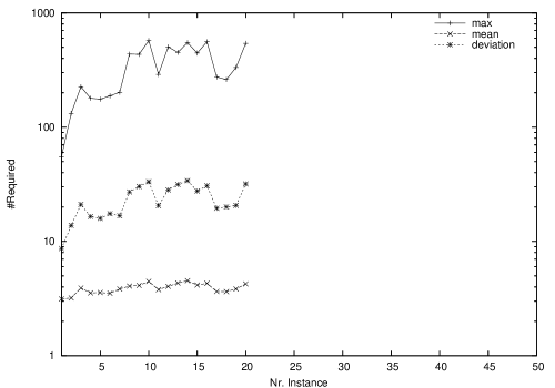
(c)	(d)

Figure 12: Distributions of the numbers of actions adding a fact, and of actions requiring a fact, in PSR “small” and “large”: (a) adders “small”, (b) requirers “small”, (c) adders “large”, (d) requirers “large”.

Data for PSR are shown in Figure 12. Here, we show plots for adders and requirers separately because that makes them much more readable. Since the data contain some particularly interesting phenomena, we show it for two domain versions, “small” and “large”. The most obvious feature in “small”, Figure 12 (a) and (b), is, once again, the huge amount of variance in the data. The clearly discernible peaks in the curves (instance nrs. 15, 25, 31, and 40) coincide with the peaks in size as measured by numbers of facts and actions in Figure 4. We also note that there is a very large range of values, spanning four orders of magnitude, even though the instances are (except number 25) all very small in comparison to the other domains shown in Figure 4. The minimum numbers of adders and requirers are constantly $1$: “updated(breaker)” is added only by a “wait(breaker)” action, “not-closed(breaker)” is only needed if one wants to close it. Regarding the maximum adders and requirers, in instance 25, which has by far the highest (9400) total number of actions, $max$ adders (9216) is due to the “goal-reached” fact, i.e., to the 9216 disjuncts in the DNF of the goal formula; $max$ requirers (9251) is due to “do-normal”, which is a flag needed for every goal-reached action, plus the actions opening or closing breakers. We remark that the same facts are responsible for all of the peaks in the curves, i.e., the same happens also in instances 15, 31, and 40.

It is highly characteristic for PSR “small” that the $max$ numbers of adders and requirers approach and sometimes exceed two thirds of the total number of actions. This is not the case for any other domain, not even for any other domain version of PSR (see below). The intuitive reason lies in one of the pre-compilation steps that we employed in order to be able to formulate reasonably large PSR instances in pure STRIPS: the compilation step (?) “removes” network reasoning (and with it, the need for derived predicates) by basically enumerating the breaker configurations and their effects on the flow of current in the network. The result is a very dense structure where each end of the network directly affects every other end, explaining the very high degree of fact connectivity, in particular explaining the extremely complex goal formulas in the four “peak” cases mentioned above.

The pre-compilation step is also the key to understanding the huge difference between the behavior in “small”, and in “large”. The latter is shown in Figure 12 (c) and (d). There, the $max$ adders curve is a small linear function – note the non-logarithmic scale of the $y$ axis – in spite of the (mostly) much larger numbers of actions. For example, the instance with the highest number (7498) of actions and derivation rules is number 20, where the $max$ number of adders is 31, less than half a percent of the total number of actions. In the natural high-level domain encoding that we have here, the flow of current through the network is modelled as the transitive closure over derivation rules that each propagate current based on the local status of the network. So in particular the breaker configurations and their effects on the flow of current are implicit in the structure of the network.

Once again, in PSR “large”, the $min$ curves are constantly $0$ for both adders and requirers; “not-affected(breaker)” is the negation of a derived predicate (needed as precondition of open and close actions), which isn’t added by an inverse rule, but given its meaning through the negation as failure semantics of derived predicates; “fed(line)” is only required for the goal. The $mean$ and $dev$ of the adders are completely flattened by the numerous (5029 out of 5237, in instance 20) “upstream(x,y)” facts, true if there is currently a path open from a side of node x to a side of node y, that are added only by a local derivation rule that relies on the same predicate for the neighbors of y. Similarly to Satellite, the $max$ number of requirers is generally a lot larger than the $max$ number of adders. For example, 542 vs. 31 in instance 20, where $max$ requirers is due to a fact “closed(device)” that is required in derivation rules talking about pairs of devices; in instance 20, 7360 of the 7498 actions are such rules; there are 46 devices.

(a)	(b)
(c)	(d)

Figure 13: Distributions of the numbers of actions adding a fact, and of actions requiring a fact, in the STRIPS versions of the IPC-3 domains except Freecell and Satellite: (a) Depots, (b) Driverlog, (c) Rovers, (d) Zenotravel.

To sum up the sub-section, the data are, generally, too abstract to be really tightly interconnected with the performance exhibited by planners. On the other hand, certain characteristics are visible. Most particularly: In Pipesworld, the numbers of adders and requirers are almost identical. In Promela, the adders are constant and the requirers are linear. In Satellite, all curves are very close together. In PSR “small” there is a lot of variance, and the $max$ numbers of adders and requirers approach and sometimes exceed two thirds of the total number of actions. In contrast, in PSR “large” the $max$ adders decline to less than half a percent of the total number of actions. In UMTS, all the parameters are constant. Except for PSR and UMTS, these phenomena are somewhat hard to interpret. If nothing else, they certainly show us that the domains have some rather different characteristics. Interestingly, the differences are not as significant for the IPC-3 benchmarks shown in Figure 13. Clearly, the behavior is not as characteristically diverse as what we have just seen for the IPC-4 domains. For all the four domains in Figure 13, we basically observe mostly parallel lines that are pretty close together except for the $max$ lines, which are about an order of magnitude higher than the others. The only striking feature is the zig-zag nature of the curves in Depots. This is due to the scaling pattern: In the smallest instances, the number of crates (blocks) grows continually up to 15 crates in instance 6. Thereafter, there come blocks of 3 instances each, of which the first has 6 crates, the second 10 crates, and the third 15 crates (across the blocks, other instance size parameters grow). This means that the zig-zag shape of the curves corresponds exactly to the zig-zag shape of the crate numbers.

Note that the behavior of the plots in Figure 13 is similar to the behavior of the plot for Satellite in Figure 11 (d), in particular for the first 20 instances. These were the instances posed to the fully automated planners in IPC-3, as also shown in Figure 13. The only IPC-3 domain that truly stands out in terms of the behavior of these curves is Freecell. There, we observe a phenomenon similar to that of the Pipesworld in Figure 11 (b), where the curves for adders and requirers almost coincide. The phenomenon is a little weaker than in Pipesworld: in the largest Freecell instance, number 20, the $max$ of (both) adders and requirers is $1638$, while the $max$ of the difference is $102$, with a $mean$ of $14.30$ and $dev$ of $24.86$. For comparison, in the largest Pipesworld instance, $max$ adders is $1524$, $max$ requirers is $1520$, and the $max$ of the difference is $29$, with a $mean$ of $1.63$ and $dev$ of $5.31$.

To sum up the overall empirical analysis, the data certainly don’t solve the mystery of what is behind the performance of every planner in every domain (and instance). They do, however, provide some interesting insights about how instances are scaled in the domains, about certain subtleties and peculiarities of their encodings, and about how standard heuristic methods, and groups of planners, react to them. We can observe large characteristic differences between the domains. In that sense the results nicely complement the technical descriptions in Appendix A, as well as the known theoretical results from Section 4.

6 Conclusion

In a field of research about general reasoning mechanisms, such as AI planning, it is essential to have useful benchmarks: benchmarks that reflect possible applications of the developed technology, and that help drive research into new and fruitful directions. In the development of the benchmark domains and instances for IPC-4, the authors have invested significant effort into creating such a set of useful benchmarks for AI planning.

As explained in the introduction, the three main goals we tried to achieve were 1. realism, 2. structural diversity, and 3. accessibility of the benchmarks. It is debatable to what extent these goals were achieved. To some extent, this is inherent in the conflicting nature of the goals. Accessibility of a benchmark – formulation in as simple as possible PDDL dialects – is obviously in conflict with realism. Structural diversity is also in conflict with realism since, in the time window available to create a competition benchmark set, there may not be (and has not been, in our case) a large set of suitable applications to choose from. One must make do with what’s available. We stressed on realism since the lack of realism was traditionally considered as one of the main weaknesses of AI Planning – achieving “just” structural diversity and accessibility would, in fact, have been comparatively easy (see also below). That said, to adapt the applications for the IPC we had to make many significant simplifications. Still, having derived the domains from applications, one can expect that they capture some important features even after simplification; on top of that, there is a clear path towards more realism.

We believe that the domains constitute the best possible compromise for IPC-4. To name the most distinguishing features of the domain set:

1. Airport, Pipesworld, PSR, and UMTS are derived directly from applications (Promela is a special case since the model checking instances we could encode are very simplistic). This was previously the case only for the Elevator domain (IPC-2) and the Rovers and Satellite domains (IPC-3).

2. The complexity of satisficing and optimal planning in the STRIPS domain versions covers the entire range P, NP, and PSPACE – deciding (bounded) plan existence is in P for PSR and PSPACE-complete for Airport and general Promela. We are not aware of a previous PSPACE-complete STRIPS benchmark; the polynomial algorithm for finding plans in PSR is, in contrast to those for all the other STRIPS benchmarks with such algorithms, quite non-trivial.

3. In Hoffmann’s (?) taxonomy of domain classes with different $h^{+}$ topology, the IPC-4 domains lie in classes with sparse coverage by previous benchmarks. In particular, none of our new domains has nearly as simple a topology as proved by Hoffmann for most of the traditional benchmarks. When taking into account that Pipesworld actions can be inverted in (not one but) two steps, each of the domains lies in a different class of Hoffmann’s taxonomy, covering more classes (6) than any previous IPC benchmark set (3, 5, and 4 for IPC-1, IPC-2, and IPC-3, respectively). Dining Philosophers is exceptional in that it lies in a “simple” class but doesn’t have a simple topology; Airport is exceptional in that it lies in a “very hard” class but is typically (in real-world instances) easy.

4. The behavior of the different kinds of planners in IPC-4 shows a lot of very characteristic patterns in the individual domains. In Airport, sheer size is the main obstacle. In Pipesworld, particularly with tankage restrictions, the known heuristic functions do very badly. In the Promela domains, the main obstacle is, in a lot of cases, the impossibility of compiling the PDDL description into a fully grounded simpler representation. In PSR, there is an extremely large amount of variance, and optimal planners perform just as well (or poorly) as satisficing planners. In UMTS, satisficing planners need no time at all.

5. At a very abstract level that just looks at the numbers of actions adding/needing each fact, the behavior of the domains is more characteristically diverse than that of the IPC-3 domains.

6. Last but not least, the STRIPS versions of our domains preserve much more of the original domain structure than what was previously the case. The IPC-2 STRIPS version of Elevator is hardly an elevator problem anymore, and the IPC-3 STRIPS versions of Satellite and Rovers are devoid of all of the more interesting problem constraints. In contrast, the STRIPS versions of Airport and Promela are semantically identical to the ADL versions, and the PSR STRIPS version, while pre-compiled a lot, still preserves much of the original difficulty of the domain (judging, e.g., by the behavior of the IPC-4 planners in it).

Feature 1 is, obviously, a point for realism. Features 2 to 5 are points for diverse structure; particularly Feature 4 shows how the domains pose very different challenges to (current) planning technology. Feature 6 is a point for realism combined with accessibility. We would like to stress that accessibility in this respect is really quite important. Of the 19 planners entered into IPC-4, only 8 could handle (some) ADL features. Our compilation approach enabled us to confront the other 11 planners with reasonably realistic problems. That said, it certainly is debatable what role STRIPS plays or should play for the community. Some people may say that many of the core algorithms, e.g., planning graphs (?) and relaxed plan heuristics (?, ?, ?), have been invented in STRIPS. Others may say that the focus on STRIPS-like languages and algorithms distracts us from considering temporal and numerical problems of a truly different nature. This notwithstanding, STRIPS is still the most widely used language among the research community. This cannot be ignored by competition organizers.

Having pointed out the advantages of our benchmark set, we should also point out a few of the disadvantages. As explained in detail in the individual sections in Appendix A, we had to make many simplifications in order to make the applications fit for use in IPC-4. To some extent, whether or not the simplifications preserve the original domain structure is a debatable matter. We feel that our Airport encoding is very close to the real “physical” thing. Not being able to represent the real optimization criterion is bad, but ameliorated by the fact that, out of 19 planners, only a single one (LPG-td) could actually deal with user-defined optimization criteria. In Pipesworld, the simplifications are more severe. The IPC-4 domain still resembles some of the core difficulties, but is more reminiscent of a (complicated) toy example than of software that could be used to control real pipelines. The Promela examples go to show that toy examples in the model checking area are not any better than the traditional toy examples in planning. In PSR, removing the uncertainty and the numerical optimization renders the IPC-4 domain unsuitable for practical use.

Of course, the domain set is not exhaustive, meaning that there presumably are numerous applications whose essential structure is not similar to any of the IPC-4 domains. Some examples that spring to mind are action choice in autonomous robots, detecting security holes in computer networks (?), and online manufacturing (?). As for structural diversity, it would be easy to construct a set of artificial domains that explore more of the possible extreme cases. Such domains would probably be completely infeasible for current planners, thus posing very strong challenges. Just think of, for example, Rubik’s Cube, Sokoban, or Rintanen’s (?) purely randomly generated instance distributions. Then again, such a domain set would be devoid of realism. At some point during the preparation of IPC-4, we considered introducing a separate class of domains, called “Diverse Structure”, which would have contained domains of this sort. We decided to not do so since the competition event was already very large without it. Also, we felt that our applications were already quite diverse on the structural side. As pointed out above, several theoretical and empirical phenomena suggest that the latter is indeed the case.

During our work, we experienced various successes and failures in accurately formulating our application domains in PDDL. People have asked us if, through this, we obtained a picture of how suitable PDDL is, in its current form, to formulate applications, and in what sorts of domains it works well. The answer is, we don’t feel like we obtained many insights into these matters that are particularly deep or haven’t been known before. A few lessons learned are these. First and foremost, formulating an application in STRIPS takes a huge amount of engineering expertise unless one just drops all problem constraints; some simplifications are unavoidable. Second, the discrete nature of action instantiations in all previous IPC PDDL dialects seriously impedes formulation of domains with continuous aspects. A discretization must be chosen, which is sometimes easy (Airport) and sometimes very hard (Pipesworld) to do. A good way out seems to be to adopt the “duration inequalities” suggested by ? (?). Third, the community should pay more attention to lifted encodings, and how to deal with them in modern planning algorithms: one lesson from our compilation activities is that grounding out all parameters is often simply not possible (Promela, PSR). Since compiling away ADL constructs is often not feasible without grounding (c.f. Section 2), this is also very relevant in the ADL/STRIPS context. As a final “lesson”, we (the AI Planning community) are still, mostly, far away from as-is applicability of planners in the real world. But we are on the right track.

To conclude, we spent significant time and effort creating a useful set of planning benchmarks for IPC-4. We hope that they will become standard benchmarks in the coming years.

Acknowledgements. We would like to thank the competitors for their detailed comments about bugs found in our domains, and we would like to thank Malte Helmert for various useful tools that helped remove some of these bugs.

We further thank Malte Helmert for providing us with his – yet unpublished, at the time of writing – results on computational complexity (?, ?). We thank Patrik Haslum for providing us with the TP4 temporal numerical plan graph estimates of makespan in the UMTS domain. We are indebted to the anonymous reviewers, and very much to David Smith and Maria Fox, whose detailed and extensive comments contributed greatly to the development of this paper. We finally thank David Smith for his extensive advice on language, including some corrections even for these very acknowledgements.

Jörg Hoffmann thanks Wolfgang Hatzack for his support in the development of the Airport domain and benchmark instances.

Frederico dos Santos Liporace is supported by Conselho Nacional de Desenvolvimento Científico e Tecnológico, Brazil. He would like to acknowledge the support of his PhD supervisor, Ruy Milidiu, in the development of the Pipesworld application.

Sylvie Thiébaux thanks Piergiorgio Bertoli, Blai Bonet, and John Slaney for their contributions to the development of the PSR domain and instances. She also would like to acknowledge the support of National ICT Australia. NICTA is funded through the Australian Government’s backing Australia’s Ability initiative, in part through the Australian Research Council.

A Detailed Domain Descriptions

We now provide detailed descriptions of all the domains, in alphabetical order. Each section (except those for the Satellite and Settlers domains, which were adapted from the IPC-3) is organized in sub-sections as follows. We first give an outline of the application domain. We then explain the main adaptations made to model the application as a PDDL domain in IPC-4, we explain the IPC-4 domain structure, i.e., the domain versions and their formulations as used in IPC-4, and we explain how we generated the example instances for the IPC-4 test suites. Finally, we discuss possible future extensions.

A.1 Airport

We had a contact person for this application domain, Wolfgang Hatzack, who has been working in this application area for several years. The domain was adapted for IPC-4 by Jörg Hoffmann and Sebastian Trüg.

A.1.1 Application Domain

The task is to control the ground traffic on an airport. Timed travel routes must be assigned to the airplanes so that they reach their targets. There is inbound and outbound traffic; the former are airplanes that must take off (reach a certain runway), the latter are airplanes that have just landed and have to get parked (reach a certain parking position). The main problem constraint is, of course, to ensure the safety of the airplanes. This means to avoid collisions, and also to prevent airplanes from entering the unsafe zones behind large airplanes that have their engines running. The optimization criterion is to minimize the summed up travel time (on the surface of the airport) of all airplanes. There usually are standard routes, i.e., routes that any airplane outbound from a certain park position area, or inbound from a certain runway, must take. The reason for introducing such routes is, simply, the sheer complexity of managing the situation otherwise, without significant computer support (which is as yet not available on real airports). We will see below that whether or not standard routes are present makes a big difference also computationally.

The airplanes move on the airport infrastructure, which consists of runways, taxiways, and parking positions. The runways and taxiways are sub-divided into smaller segments. The position of an airplane is given by the segment it is currently located in, plus its direction and the more precise position within the segment – several airplanes can be in the segment at the same time.

Airplanes are generally divided into three categories, light, medium, and heavy, which classify them according to their engine exhaust (jet blast). An airplane that has to be moved is either in-bound or out-bound. In-bound airplanes have recently landed and are on their way from the runway to a parking position, usually a gate. Out-bound airplanes are ready for departure, meaning they are on their way to the departure runway. Since airplanes cannot move backwards, they need to be pushed back from the gate onto the taxiway, where they start up their engines. Some airports also provide different park positions that allow an airplane to start its engines directly.

To ensure safety, an airplane must not get too close to the back of another airplane whose engines are running. How far the safety distance has to be depends on the category (jet blast) of the second airplane.

The ground controller – the planner – has to communicate to the airplanes which ways they shall take and when to stop. While such guidance can be given purely reactively, it pays off to base decisions on anticipating the future. Otherwise it may happen that airplanes block each other and need more time than necessary to reach their destinations on the airport. The objective is, as said, to minimize the overall summed up traveling times of all airplanes.

As instances of the domain, one considers the traffic situation at some given point in time, with a time horizon of, say, one hour. If new airplanes are known to land during given time slots inside the time horizon, then during these time slots the respective runways are considered blocked, and the planner has to make sure these runways are free at these times. Of course, because the situation changes continually (new planes have to be moved and plans cannot be executed as intended), continuous re-planning, i.e., consideration of the domain instance describing the new traffic situation, is necessary. Solving instances optimally (the corresponding decision problem) is PSPACE-complete without standard routes (?) and NP-complete if all routes are standardized (?). In the latter case, we have a pure scheduling problem. In the former case, complicated (highly unrealistic, of course) airport topologies can lead to exponentially long solutions, c.f. Section 4.1.

A.1.2 IPC-4 PDDL Adaptation

The PDDL encoding (as well as our example instance generation process, see below) is based on software by Wolfgang Hatzack, namely on a system called Astras: Airport Surface ground TRAffic Simulator. This is a software package that was originally designed to be a training platform for airport controllers. Astras provides a two-dimensional view of the airport, allowing the user to control the airplanes by means of point and click. Astras can also simulate the traffic flow on an airport over the course of a specified time window.

We made three simplifications, one of them benign, to the airport model. As for the benign simplification: we did not model park positions where the airplane can start up its engines directly, without being pushed back to the taxiway first. While it is not difficult to model such park positions in PDDL, they seldom occur in reality and so are not very relevant to the application. Our first more important simplification was to assume a somewhat cruder notion of airplane locatedness, by requiring that only a single airplane can be located in a segment at any time. That is, we use the term “segment” with the meaning of a smallest indivisible unit of space. To minimize the loss of precision, (some of) the original “segments” were sub-divided into several new smaller segments. The safety distance behind the back of an airplane whose engines are running is then also measured in terms of a number of segments. While this discretization makes us lose precision, we believe that it does not distort the nature of the problem too much: due to the amount of expected conflicting traffic at different points on the airport (high only near parking positions), it is relatively easy to choose a discretization – with segments of different length – that is precise and small enough at the same time. The last simplification is more severe. We had to give up on the real optimization criterion. We say more on this rather strong simplification below. We did not use full standard routes, thus allowing the airplanes a choice of where to move. We did use standards for some routes, particularly the regions near runways in large airports. For one thing, this served to keep large airports manageable for the PDDL encoding and planners; for another thing, it seems a good compromise at exploiting the capabilities of computers while at the same time keeping close to traditions at airports. We get back to this matter in Section A.1.5.

The full PDDL description of our domain encoding can be downloaded from the IPC-4 web page at http://ipc.icaps-conference.org/. Briefly, the encoding works as follows. The available actions are to “pushback” (move a plane away backwards from a parking position), to “startup” the engines, to “move” between segments, to “park” (turning off the engines), and to “takeoff” (which amounts to removing the plane from the airport). The semantics of these actions are encoded based on predicates defining the current state of the airplane. At any point in time, an airplane is either moving, pushed, parked, or airborne. An airplane always occupies one segment and, if its engines are running, may block several other segments depending on the size of the occupied segment and the category of the airplane. The action preconditions ensure that blocked segments are never occupied by another airplane. In the initial state, each plane is either parked, or moving. A parked plane can be pushed back, and after starting up its engines, it is moving. A moving airplane can either move from its current segment to a neighboring segment, park – at a parking position – or take off – on a runway.

As an example, have a look at the PDDL encoding of the (non-durational) “move” action (one of the preconditions was used as an example in Section 2 already):

(	:action move
	:parameters
	(?a - airplane ?t - airplanetype ?d1 - direction ?s1 ?s2 - segment ?d2 - direction)
	:precondition
	(and	(has-type ?a ?t) (is-moving ?a) (not (= ?s1 ?s2)) (facing ?a ?d1) (can-move ?s1 ?s2 ?d1)
		(move-dir ?s1 ?s2 ?d2) (at-segment ?a ?s1)
		(not (exists (?a1 - airplane) (and (not (= ?a1 ?a)) (blocked ?s2 ?a1))))
		(forall (?s - segment) (imply (and (is-blocked ?s ?t ?s2 ?d2) (not (= ?s ?s1))) (not (occupied ?s)))))
	:effect
	(and	(occupied ?s2) (blocked ?s2 ?a) (not (occupied ?s1)) (not (at-segment ?a ?s1)) (at-segment ?a ?s2)
		(when (not (is-blocked ?s1 ?t ?s2 ?d2)) (not (blocked ?s1 ?a)))
		(when (not (= ?d1 ?d2)) (and (not (facing ?a ?d1)) (facing ?a ?d2)))
		(forall (?s - segment) (when (is-blocked ?s ?t ?s2 ?d2) (blocked ?s ?a)))
		(forall	(?s - segment) (when
			(and (is-blocked ?s ?t ?s1 ?d1) (not (= ?s ?s2)) (not (is-blocked ?s ?t ?s2 ?d2)))
			(not (blocked ?s ?a))))))

The six parameters – which is a lot compared to most of the usual benchmarks – do not cause a prohibitive explosion in instantiations since there is a lot of restriction through static predicates. Airplane “?a” moves; its type (category) is “?t”; it is at segment “?s1” facing in direction “?d1”, and will be at “?s2” facing in direction “?d2” after the move. “Direction” here is a very simple concept that just says which end of the segment the airplane is facing. Of course, moves from “?s1 ?d1” to “?s2 ?d2” are only possible as specified by the – static – topology of the airport (“can-move”, “move-dir”). The first of the two more complex preconditions says that “?s2” must not currently be blocked by any airplane other than “?a” itself. The second complex precondition makes sure that, after the move, “?a” will not block a segment that is currently occupied (by another airplane, necessarily): “(is-blocked ?s ?t ?s2 ?d2)” is a static predicate that is true iff “?s” is endangered – blocked – if a plane of type “?t” is at “?s2”w facing direction “?d2”. The effects should be self-explanatory; they simply update the “at”, “occupied”, and “blocked” information. The only effect that looks a little complicated – the last one – says that those segments that were blocked before the move, but are no longer blocked after the move, become un-blocked. Note that the conditions of all conditional effects are static, so the conditions disappear once the parameter instantiation is chosen.

In durational PDDL, the actions take time according to some simple computations. The time taken to move across a segment depends, naturally, on the segment length and the speed. We assumed that airplanes move at the same speed regardless of their category. The time taken to start up the engines is proportional to the number of engines. The other actions have some fixed duration.

If some planes are known to land in the near future, blocking runways, then we model the blocking during these time windows using timed initial literals, respectively their compilation into artificial (temporal) PDDL constructs. The timed literals are simply instances of the usual “blocked” predicate, becoming true when the respective time window starts, and becoming false again when it ends.

We were not able to model the real optimization criterion of airport ground traffic control. The standard criterion in PDDL is to minimize the execution time, i.e., makespan, of the plan. In our encoding of the domain this comes down to minimizing the arrival time (meaning, arrival at the destination on the airport) of the last airplane. But the real objective is, as said above, to minimize the overall summed up travel time of all airplanes. There appears to be no good way of modeling this criterion in current PDDL. The difficulty lies in accessing the waiting times of the planes, i.e. the times at which they stay on a segment waiting for some other plane to pass.

The only way (we could think of) to get access to the waiting times, in current PDDL, is to introduce an explicit waiting action. But then one must be able to tell the planner, i.e., to encode in the action, how long the plane is supposed to wait. One option is to use the “duration inequalities” proposed by ? (?). There the action imposes only some constraints on its duration, and the planner can/has to choose the actual duration of the action, at each point where it is used in the plan, as an additional (rational-valued) parameter. The potential disadvantage of this approach is that the choice of the waiting time introduces, in principle, an infinite branching factor into the state space, and may thus make the problem much harder for automated planners. Moreover, duration inequalities were not put to use in IPC-3, and were not a part of PDDL2.1. When not using duration inequalities, the only way to encode the requested waiting time into the action is to use a discretization of time. One can then introduce new objects representing every considered time interval, and give the waiting action a parameter ranging over these objects. Apart from the loss of precision involved in the discretization, this approach is also likely to cause huge performance problems for automated planners. As an alternative way out, we considered introducing a special “current-time” variable into PDDL2.2, returning the time of its evaluation in the plan execution. Using such a “look at the clock”, one could make each plane record its arrival time, and thus formulate the true optimization criterion without any major changes to the domain structure. The IPC-4 organizing committee decided against the introduction of a “current-time” variable as it seemed to be problematic from an algorithmic point of view (it implies a commitment to precise time points at planning time), and didn’t seem to be very relevant anywhere except in Airport.

All in all, the IPC-4 PDDL encoding of the Airport domain is realistic except for the optimization criterion, which demands to minimize maximal arrival time – makespan – instead of summed up travel time. It remains to remark that all but one (LPG-td) of the IPC-4 planners ignored the optimization criterion anyway. Also, minimizing the latest arrival time does appear a useful (if not ideal) objective.

A.1.3 IPC-4 Domain Structure

The Airport domain versions used in IPC-4 are non-temporal, temporal, temporal-timewindows, and temporal-timewindows-compiled. The first of these versions is, as the name suggests, non-durational PDDL. In the second version, actions take time as explained above. The third and fourth versions also consider runways blocked in the future by planes known to land during given time windows. The third version encodes these time windows using timed initial literals, the fourth version uses those literals’ compilation into standard temporal PDDL constructs, c.f. Section 2.

In all the domain versions, the problem constraints are modeled using ADL, i.e., complex preconditions and conditional effects. We compiled the ADL encodings to STRIPS with domain-specific software implemented for this purpose. We grounded out most – not all – of the operator parameters, precisely, all the parameters except, for each action, the one giving the name of the affected individual airplane. Once all the other parameters are fixed, the formulas and conditional effects can be simplified to the usual STRIPS constructs. Each Airport domain version contains the original ADL formulation, as well as its compilation to STRIPS. The result of the grounding process depends on the specific airport considered in the instance, and on the set of airplanes that are travelling. So, in the STRIPS formulations, to each instance there is an individual domain file (the same applies to all STRIPS compilations in the other domains described later).

The domain versions, as well as the blow-up incurred by the compilation, are overviewed in Table 1. The numbers shown in the table indicate numbers of PDDL operators, and numbers of grounded actions. For each domain version/formulation, the maximum such number of any instance is shown. Note that, in the ADL formulations except temporal-timewindows-compiled, there is just a single domain file so the number of operators is identical for all instances. In the STRIPS formulations, the number of operators is high because, as explained, most of the operator parameters are grounded. The difference in the number of ground actions between the STRIPS and the ADL formulations is because, with our automated software, we were not able to generate the ground actions in the larger ADL instances; the data shown are for the largest instances that we could handle. The numbers shown in parentheses refer to the situation before FF’s “reachability” pre-process; as said before, this builds a relaxed planning graph for the initial state, and removes all actions that do not appear in that graph. The difference between the numbers inside and outside of the parentheses indicates how much this simple pre-process helps. We see that it helps quite a lot here, pruning almost half of the actions (which would never become applicable, in a forward search at least, but which blow up the representation regardless of what algorithm is used).

version	formulation	$max\mbox{-}\#op$	$max\mbox{-}\#act$
non-temporal	ADL	5	(1048) 989
non-temporal	STRIPS	1408	(21120) 13100
temporal	ADL	5	(1408) 989
temporal	STRIPS	1408	(21120) 13100
temporal-tw	ADL	5	(995) 854
temporal-tw	STRIPS	1408	(22038) 13100
temporal-twc	ADL	14	(911) 861
temporal-twc	STRIPS	1429	(21141) 13121

Table 1: Overview over the different domain versions and formulations of Airport. Abbreviations used: “temporal-tw” for “temporal-timewindows”, “temporal-twc” for temporal-timewindows-compiled; $max\mbox{-}\#op$ is the maximum number of (parameterized) PDDL operators for any instance, $max\mbox{-}\#act$ is the maximum number of ground actions for any instance. For the ADL formulations, the set of ground actions could not be generated for the largest instances; data are shown for the largest instances that could be handled. Data in parentheses are collected before FF’s “reachability” pre-process (see text).

A.1.4 IPC-4 Example Instances

The Airport example instances were generated by Sebastian Trüg, with an implementation based on the aforementioned airport simulation tool Astras. Five scaling airport topologies were designed, and used as the basis for the instance generation. The airports are named “Minimal”, “Mintoy”, “Toy”, “Half-MUC”, and “MUC”. The smallest of these airports is the smallest possible airport Astras can handle. The two largest airports correspond to one half of Munich Airport (MUC), and to the full MUC airport. Figure 14 shows sketches of the “Minimal” airport, and of the “MUC” airport.

(a)

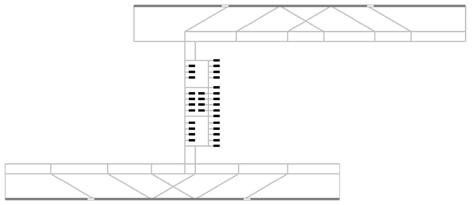
(b)

Figure 14: The smallest (a), and the largest (b) of the IPC-4 Airport topologies. Park position segments are marked in black (e.g., at the top of part (a)), while the segments airplanes can takeoff from are marked in white (e.g., at the left bottom side of part (a)). The lines show the road network on the airport. Topology (b) corresponds to MUC airport.

Sebastian Trüg implemented PDDL instance generation software inside Astras. During a simulation of the traffic flow on an airport, if desired by the user the software exports the current traffic situation in the various PDDL encodings explained above. The simulator was run with the different airports, and 50 scaling traffic situations were exported (3 on “Minimal”, 6 on “Mintoy”, 11 on “Toy”, 15 on “Half-MUC”, and 15 on “MUC”). For each airport, the instances scale in terms of the number of travelling airplanes. The largest instance features 15 planes to be moved to their destinations on Munich airport, with 10 planes landing in the future to be considered (in the respective domain versions). This can be considered a realistically sized traffic situation, at this airport.

A.1.5 Future Work

It remains to explore how to relax some of the simplifications we had to make. Most importantly, how to overcome the discrete model of space (locatedness), and how to model the real optimization criterion. Our difficulties with both are, as partly described above already, mostly due to the discrete nature of PDDL2.2, which does not allow a continuous choice in the instantiation of an action. Such a continuous choice would be the most natural way of saying how far a plane will be moving and how long it will be waiting. So the best way to go about this direction is, probably, to assume the “duration inequalities” proposed by ? (?), together with the numeric variables already contained in PDDL2.2. This should be easy on the modelling side. The main problem is probably on the technology side, i.e., to develop planners that can deal efficiently with such continuous choice points. At the time of IPC-4, as said, continuous choice appeared too much to demand from the planners.

One interesting topic for future work arises if one restricts the airplanes completely to standard routes, i.e., leaves them no choice at all of what route to take to their destination. As said, first, this is usually done at real airports, for the sheer complexity of managing the situation otherwise, without significant computer support (which is as yet not available at real airports). Second, in IPC-4 we made only limited use of this feature, to retain some of the flexibility that could be offered by automatized methods. Third, the restriction turns the PSPACE-complete ground traffic control problem into a pure, NP-complete (?), scheduling problem, where the only question is when the planes move across what segment. One could exploit this to create a much more concise PDDL encoding. The restricted problem comes down to resolving all conflicts that arise when two planes need to cross the same airport segment. One could thus try to not encode in PDDL the physical airport, but only the conflicts and their possible solutions, ideally in connection with the real optimization criterion. It can be expected that planners will be much more efficient in such a simpler and more concisely encoded problem.

A.2 Pipesworld

Frederico Liporace has been working in this application area for several years; he submitted a paper on an early domain version to the workshop on the competition at ICAPS’03. The domain was adapted for IPC-4 by Frederico Liporace and Jörg Hoffmann.

A.2.1 Application Domain

Pipelines play an important role in the transportation of Petroleum and its derivatives, since it is the most effective way to transport large volumes over large distances. The application domain we consider here deals with complex problems that arise when transporting oil derivative products through a multi-commodity pipeline system. Note that, while there are many planning benchmarks dealing with variants of transportation problems, transporting oil derivatives through a pipeline system has a very different and characteristic kind of structure, since it uses stationary carriers whose cargo moves rather than the more usual moving carriers of stationary cargo. In particular, changing the position of one object directly results in changing the position of several other objects. This is less reminiscent of transportation domains than of complicated single-player games such as Rubic’s Cube. It can lead to several subtle phenomena. For example, it may happen that a solution must reverse the flow of liquid through a pipeline segment several times. It may also happen that liquid must be pumped through a ring of pipeline segments in a cyclic fashion, to achieve the goal (we will see an example of this later).

In more detail, the application domain is the following. A pipeline network is a graph of operational areas connected by pipeline segments. Operational areas may be harbors, distribution centers or refineries. These may be connected by one or more pipeline segments. The oil derivatives are moved between the areas through the pipelines.

There can be different types of petroleum derivative products. Each area has a set of tanks that define the storage capacity for each product type. Each pipeline segment has a fixed volume and speed. The volume depends on the segment’s length and cross section diameter, and the speed depends on the power of the pumps that move the contents. A segment may be uni-directional, i.e. only usable for transportation in one direction.

Pipeline segments are always pressurized, that is, they must be always completely filled with petroleum derivative products. Because of that, the only way to move a pipeline segment’s contents is by pumping some amount of product from an adjacent area into the segment. This operation results, assuming incompressible fluids, in the same amount of a possibly different product being received in the area at the other end of the segment.

The pumping operations can only be executed if they do not violate any interface or tanking constraints. As for the former, distinct products have direct contact inside the pipeline segment, so it is unavoidable that there is some loss due to the mixture in the interface between them. These interface losses are a major concern in pipeline operation, because the mixed products can not be simply discarded. They must pass through a special treatment that may involve sending them back to a refinery, and that may require the use of special tanks. The severity of interface losses depends on the products that interface inside the pipeline segment. If two product types are known to generate high interface losses, the pipeline plan must not place them adjacently into the segment. Such a pair of product types is said to have an interface restriction.

Tanking constraints are limits on the product amounts that can be stored in an area, arising from the respective tank capacities. Such constraints may effectively block a pipeline segment, if there is no room in the receiving area to store the product that would leave the segment in the process of a pumping operation.

The task in the application is to bring certain amounts of products to the areas in which they are required, i.e. one has to find a plan of pumping operations that shifts the positions of the product amounts in a way so that the goal specifications are met. Sometimes there is a deadline specifying when, at the latest, a product amount has to arrive at its destination area. It may also be the case that an area (typically, a refinery) is known to produce some given amount of a product at a given point in time, and that the plan must make sure that there is enough tank space available at the respective area to store the new product amount. Similarly, an area (typically, a harbor or a distribution center) may be known to consume some given amount of a product at a given point in time, thereby freeing the respective amount of tank space.

A.2.2 IPC-4 PDDL Adaptation

The main adaptations made in the PDDL encoding are unitary batches, split pumping operations, and “personalized” goals (see below for the latter). The term “batch” is used in the oil pipeline industry to refer to an amount of a product that must be transported through the pipeline. Batches are thus associated with a single product and have predefined volume. Batches are also indivisible. When a batch $B_{i}$ is pumped from an area $A_{j}$ into a segment $S_{j,k}$, it is not possible for another batch to be pumped from $A_{j}$ into $S_{j,k}$ until all of $B_{i}$’s volume is pumped. Of course, in reality the product amount in a batch is a rational number. Using such a numeric encoding in IPC-4 seemed completely infeasible due to complications in the modeling, and the expected capabilities of the participating planners (see Section A.2.5). Instead, we based the encoding on the concept of what we called unitary batches. These are the smallest considered – indivisible – portions of product. The pumping operations refer to unitary batches. The pipeline segments’ volumes and the volumes of tanks are also defined in terms of unitary batches. When encoding a real-world instance of the domain, the actual volume associated with a unitary batch is a choice variable. Smaller unitary batches decrease the rounding error in the PDDL encoding, at the cost of a larger encoding size. Note that, like the smallest units of space in the Airport domain, this is a discretization the need for which is due to the non-continuous nature of actions in PDDL2.2; we get back to this in Section A.2.5.

We modeled pipe segments in a directional fashion, i.e. there is a default direction assigning one area the “from” role, and the other area the “to” role. The pumping operations accordingly distinguish between “push” actions, which move liquid in the respective segment’s default direction, and “pop” actions, which move liquid in the opposite direction. This is simply a technical device to enable the encoding of the pipe segment contents through predicates defining the “first” and “last” batches in the segments (as well as a “successor” relation). The “push” and the “pop” actions receive (amongst other things) as arguments the pipeline segment whose contents are being moved, and the batch that is being inserted into the segment. The batch that leaves the segment depends on the segment content before the action is executed. Figure 15 shows an example.

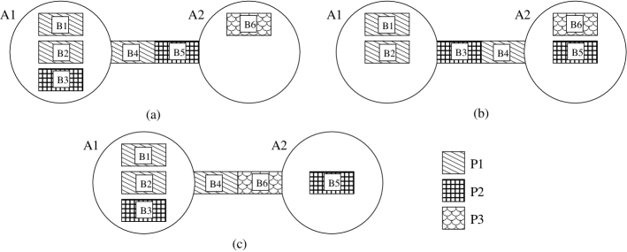
Figure 15: A small example. A1 plays the “from” role. The fill pattern for each batch represents its product. (a) shows the initial state, (b) shows state (a) after a “push” operation with B3 being inserted into the segment, (c) shows state (b) after a “pop” operation with B6 being inserted into the segment.

Apart from the pipe segment and the batch being inserted, the “push” and “pop” actions have to take several more parameters regarding, e.g., product types and tank slots. In particular, in order to be able to update the segment contents correctly, the actions also need parameters giving the respective first, last, and second last batch in the current contents of the segment. Thus such an action has four parameters ranging over batches, yielding at least $n^{4}$ ground instances of the action when there are $n$ (unitary) batches in the considered task. We found that this made the domain completely infeasible for any planning system that grounded out the actions. Since many unitary batches are needed to encode even relatively small Pipesworld examples, such planners typically died in the pre-processing phase already. We avoided this phenomenon by splitting the actions into two parts, a “start” action taking as batch parameters only the inserted batch and the first batch in the pipe, and an “end” action taking as batch parameters only the last and second last batches in the pipe. To make this more concrete, here is the split “push” action:

(	:action PUSH-START
	:parameters
	(?pipe - pipe ?batch-atom-in - batch-atom ?from-area - area ?to-area - area
	?first-batch-atom - batch-atom ?product-batch-atom-in - product
	?product-first-batch - product)
	:precondition
	(and	(normal ?pipe) (first ?first-batch-atom ?pipe) (connect ?from-area ?to-area ?pipe)
		(on ?batch-atom-in ?from-area) (not-unitary ?pipe)
		(is-product ?batch-atom-in ?product-batch-atom-in)
		(is-product ?first-batch-atom ?product-first-batch)
		(may-interface ?product-batch-atom-in ?product-first-batch))
	:effect
	(and	(push-updating ?pipe) (not (normal ?pipe)) (first ?batch-atom-in ?pipe)
		(not (first ?first-batch-atom ?pipe)) (follow ?first-batch-atom ?batch-atom-in)
		(not (on ?batch-atom-in ?from-area))))
(	:action PUSH-END
	:parameters
	(?pipe - pipe ?from-area - area ?to-area - area ?last-batch-atom - batch-atom
	?next-last-batch-atom - batch-atom)
	:precondition
	(and	(push-updating ?pipe) (last ?last-batch-atom ?pipe) (connect ?from-area ?to-area ?pipe)
		(not-unitary ?pipe) (follow ?last-batch-atom ?next-last-batch-atom))
	:effect
	(and	(not (push-updating ?pipe)) (normal ?pipe)
		(not (follow ?last-batch-atom ?next-last-batch-atom))
		(last ?next-last-batch-atom ?pipe) (not (last ?last-batch-atom ?pipe))
		(on ?last-batch-atom ?to-area)))

The constructs should be largely self-explanatory. The static predicates used are: “connect”, encoding the topology of the network; “is-product”, encoding the types of liquid; “may-interface”, encoding the interface restrictions; “not-unitary”, saying whether or not a pipe segment contains just one batch – in which case the “push” and “pop” actions are much simpler and need not be split (the “first” and “last” elements in the pipe are identical). The predicates “normal” and “push-updating” ensure, in the obvious way, that the two parts of the split action can only be used as intended. Finally, “on”, “first”, “follow”, and “last” encode where the relevant batches are. The role of “on” should be clear, it just encodes locatedness in areas. As for the pipe contents, they are modelled in a queue-like fashion, with a head “first”, a tail “last”, and a successor function “follow”. The two parts of the “push” action update this representation accordingly.

We did not encode uni-directional pipe segments, i.e. for all segments both “push” and “pop” actions are available in the IPC-4 encodings. We modeled tankage restrictions with simple constructs involving tank slots located in areas, each slot having the capacity to store one unitary batch of some given product type – that is, the “push” and “pop” actions now also specify what tank slot the inserted/outgoing batch comes from/is inserted into. For simple examples regarding interface and tankage restrictions, re-consider Figure 15. If the storage capacity for $P_{2}$ in $A_{2}$ is equal to zero, then the transition from state (a) to state (b) becomes invalid. If we forbid the interface between $P_{1}$ and $P_{3}$, then the transition from state (b) to state (c) becomes invalid.

Pipe segment speed can be easily taken account of (in durational PDDL). If the speed of a segment is $s$, then simply assign the “push”/“pop” actions regarding that segment a duration proportional to $\frac{1}{s}$. (In the IPC-4 encoding, each “start”/“end” action takes exactly that time, while the non-split actions regarding length-1 segments take time $\frac{2}{s}$.)

In reality, as outlined above the goals refer to amounts of product requested to be at certain destination areas. With our encoding based on batches, formulating such a goal would mean to introduce a potentially large disjunction of conjunctive goals. If one wants to say, e.g., that three unitary batches of product $P$ are requested in area $A$, then the needed goal condition is the disjunction $\bigvee_{\{b_{1},b_{2},b_{3}\}\subseteq B}(atb_{1}A)\wedge(atb_{2}A)\wedge(atb_{3}A)$ of the respective conjunctive goal for all three-subsets $\{b_{1},b_{2},b_{3}\}$ of the batches $B$ of type $P$. To avoid exponential blow-ups of this kind, in our encoding we used “personalized” goals instead, referring to specific batches instead of product amounts. Basically, this comes down to pre-selecting one of the $\{b_{1},b_{2},b_{3}\}$ subsets in the above disjunction. One could also avoid the blow-up by replacing the disjunction with an existential quantification; but that step would be undone in the compilation to STRIPS anyway.

Deadlines on the arrival of batches are, in durational PDDL, easily modeled by their compilation to timed initial literals. For each goal deadline there is a literal saying that the respective batch can still be ejected from the end of a pipe segment. The literal is initially true, and becomes false at the time of the deadline. As described above, in the application there can also be pre-specified time points at which an area produces or consumes a given amount of a product. We did not model this in the IPC-4 domain (see also Section A.2.5).

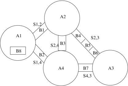
Figure 16: An example where cycling is required to achieve the goal (place B8 in A3). Pipe segment $Si,j$ is directed from $Ai$ to $Aj$.

As mentioned above, the structure of the Pipesworld domain can lead to several subtle phenomena in the possible plans. An example where plans have to perform a cyclic sequence of pumping operations is depicted in Figure 16. The goal is to place B8 in A3. The shortest plan is the following (for readability, in the action parameters only the batches going into and out of the pipes are shown): 0: PUSH S1,4 B8 B2, 1: POP S2,4 B2 B3, 2: POP S1,2 B3 B1, 3: PUSH S1,4 B1 B8, 4: PUSH S4,3 B8 B7, 5: POP S2,3 B7 B4, 6: PUSH S2,4 B4 B2, 7: PUSH S4,3 B2 B8. Observe that this plan contains two cyclic patterns. Action $0$ inserts $B8$ into $S14$. Actions $1,2,3$ then form a cycle $\{S_{2,4},S_{1,2},S_{1,4}\}$ that brings $B8$ into A4. Thereafter, action $4$ inserts $B8$ into $S43$, and actions $5,6,7$ form another cycle $\{S_{2,3},S_{2,4},S_{4,3}\}$ bringing $B8$ to its goal position $A3$.

A.2.3 IPC-4 Domain Structure

The Pipesworld domain versions used in IPC-4 are notankage-nontemporal, tankage-nontemporal, notankage-temporal, tankage-temporal, notankage-temporal-deadlines, and notankage-temporal-deadlines-compiled. All versions include interface restrictions. The versions with “tankage” in their name include tankage restrictions. In the versions with “temporal” in their name, actions take different amounts of time depending on the pipeline segment that is being moved, as explained above. The versions with “deadlines” in their name include deadlines on the arrival of the goal batches. One of these versions models the deadlines using timed initial literals, in the other version (naturally, with “compiled” in its name) these literals are compiled into artificial (temporal) PDDL constructs. None of the encodings uses any ADL constructs, and of each version there is just one (STRIPS) formulation.

version	formulation	$max\mbox{-}\#op$	$max\mbox{-}\#act$
notankage-nontemporal	STRIPS	6	(14800) 13696
notankage-temporal	STRIPS	6	(14800) 13696
notankage-temporal-d	STRIPS	6	(8172) 7740
notankage-temporal-dc	STRIPS	9	(8175) 7742
tankage-nontemporal	STRIPS	6	(107120) 101192
tankage-temporal	STRIPS	6	(107120) 101192

Table 2: Overview over the different domain versions of Pipesworld. Abbreviations used: “temporal-d” for “temporal-deadlines”, “temporal-dc” for deadlines-compiled; $max\mbox{-}\#op$ is the maximum number of (parameterized) PDDL operators for any instance, $max\mbox{-}\#act$ is the maximum number of ground actions for any instance. Data in parentheses are collected before FF’s “reachability” pre-process (see text).

The domain versions and numbers of ground actions are overviewed in Table 2. As before, the data were measured using (a temporal extension of) FF’s pre-processor. The numbers shown in parentheses refer to the situation before that pre-processor’s “reachability” pre-process, which builds a relaxed planning graph for the initial state and removes all actions that do not appear in that graph. We can observe that the numbers of ground actions are very low in the domain versions with deadlines, and extremely high in the versions with tankage restrictions. The former is simply because, due to the complicated generation process (explained in the next sub-section), examples with deadlines were generated only up to a smaller size. The latter – high numbers of actions in the presence of tankage restriction – is due to the additional blow-up incurred by the choice of tank slots from which to draw/in which to put the batches. We note that the effect of the “reachability” pruning is relatively moderate, in particular much lower than, e.g., in Airport, c.f. Section A.1.3.

A.2.4 IPC-4 Example Instances

The Pipesworld example instances were generated by Frederico Liporace, in a process going from random generators to XML files to PDDL files. Five scaling network topologies were designed and used as the basis for the instance generation. Figure 17 shows the network topologies, as well as a real-world network topology for comparison. As one can see, the largest network topology used in IPC-4 is not quite yet in the same ballpark as the real network; but neither is it trivially small in comparison. The volumes for pipeline segments that connect the same areas in the real-world example are not necessarily the same because the segments may have different cross section diameters.

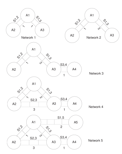
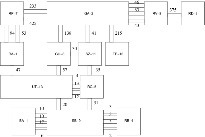
(a)	(b)

Figure 17: The IPC-4 Pipesworld network topologies (a), and a real network topology (b). The segment volumes in the latter are annotated in $100m^{3}$ units.

For the domain versions without tankage restrictions and deadlines, for each of the network topologies 10 scaling random instances were generated. Within a network, the instances scaled in terms of the total number of batches and the number of batches with a goal location. For the instances featuring tankage restrictions or deadlines, the generation process was more complicated because we wanted to make sure to obtain only solvable instances. For the tankage restriction examples, we ran Mips (?) on the respective “notankage” instances, with incrementally growing tankage. We chose each instance at a random point between the first instance solved by Mips, and the maximum needed tankage (enough tankage in each area to accommodate all instance batches). Some instances could not be solved by Mips even when given several days of runtime, and for these we inserted the maximum tankage. For the deadline examples, we ran Mips on the corresponding instances without deadlines, then arranged the deadline for each goal batch at a random point in the interval between the arrival time of the batch in Mips’s plan, and the end time of Mips’s plan. The instances not solved by Mips were left out.

A.2.5 Current and Future Work

There is ongoing work on developing a Pipesworld specific solver, named Plumber (?, ?). Plumber incorporates a pipeline simulator, domain specific heuristics, and procedures for reducing the branching factor by symmetry elimination. It also lets the user choose between different search strategies, such as enforced hill climbing (?) and learning real time A*(?). Currently it is being extended to support temporal planning as well.

The availability of this solver will enable the extension of the Pipesworld benchmark, since it will be easier to overcome the aforementioned difficulties in generating large feasible instances. We hope to be able to generate feasible instances for real-world pipeline topologies, like the one shown in Figure 17.

In addition to generating larger instances, the Pipesworld benchmark may be extended in many ways to make it closer to the real application scenario. The relevant possible extensions include:

• Defining some pipeline segments with a single flow direction, that is, segments where only “push” or “pop” actions are allowed. Note that this introduces dead ends/critical choices into the problem.

• Un-personalized goals. This could be accomplished, e.g., by imposing the desired tank volume for the goal products in the respective areas. The planner then also has to decide which batches will be used to bring the tank volume up to the desired level.

• Modeling production and consumption of products at pre-specified points in time, as described above.

• Using rational numbers to model tank capacities and current volumes, instead of the encoding based on unitary tank slots. Apart from being a more precise model of the real world (when combined with rational-valued batch sizes, see below), such an encoding would avoid unnecessary symmetries that currently arise from the availability of several non-distinguishable tank slots (in the same area, for the same product).

The most important shortcoming of our encoding is the use of unitary batches. It would be much more appropriate to base the encoding on product amounts given by real numbers. One problematic aspect of such an encoding is that it would, most naturally, demand a continuous choice of how much liquid to pump into a pipeline. Like in Airport (c.f. Section A.1.5), such a choice could naturally be modelled using Fox and Long’s (?) “duration inequalities”, but it is unclear how to develop planners that can deal with these reasonably well. Unlike in Airport, implementing such a choice is not the end of the difficulties on the modelling side. How to model the continuous contents of a pipeline? The number of distinct regions of liquid in the pipeline can grow arbitrarily high, in principle. One solution might be to fix some upper bound, and simply disallow a pumping operation if it would result in too many distinct regions. This may be a bearable loss of precision, given the upper bound is high enough. But even then, it is bound to be awkward to correctly update the contents of the pipeline when some amount $x$ of product is pushed in: the number of different products leaving the pipe depends on $x$. An option here may be to use a complicated construct of conditional effects.

All in all, our impression is that pipeline scheduling won’t be realistically modelled in PDDL, and successfully solved with planners, unless one introduces into the language a data structure suitable for modelling the contents of pipes. Basically, this would be queues whose elements are annotated with real numbers, and whose basic operations are the usual “push” and “pop”. The semantics of the pipes could then be explicitly computed inside the planner, rather than awkwardly modelled using language constructs that are likely to disturb a general search mechanism.

A.3 Promela

This domain was created for IPC-4 by Stefan Edelkamp.

A.3.1 Application Domain

Before dropping into the Promela domain, we briefly recall its origin.

The model checker SPIN (?) targets efficient software verification. It has been used to trace logical design errors in distributed systems design, such as operating systems, data communications protocols, switching systems, concurrent algorithms, railway signaling protocols, etc. The tool checks the logical consistency of a specification. SPIN reports on deadlocks, unspecified receptions and identifies race conditions, and unwarranted assumptions about the relative speeds of processes. SPIN (starting with Version 4) provides support for the use of embedded C code as part of model specifications. This makes it possible to directly verify implementation level software specifications, using SPIN as a driver and as a logic engine to verify high level temporal properties. SPIN works on-the-fly, which means that it avoids the need to construct a global state graph as a prerequisite for the verification of system properties. SPIN supports property checking in linear temporal logic (LTL). LTL expresses state trajectory constraints, using temporal modalities like eventually, always, and until. SPIN uses specific mechanisms for specifying deadlock-freeness and other safety properties, in addition to general LTL specifications. To explore the state space an ordinary or a nested search algorithm is applied, depending on whether or not a state-based (a.k.a. safety) property is to be verified.

Promela is SPIN’s input specification language. Its computational model is that of asynchronous communicating finite state machines. Promela allows to define classes of finite processes. A special process called init is started first and usually governs the instantiation of the other processes of the system. As it is possible for a process to invoke another one, Promela allows modeling systems with dynamic creation of state components. Communication in Promela is achieved via shared variables and message channels. Two kind of message channels are distinguished for synchronous and asynchronous communication. An asynchronous channel is basically a FIFO queue, while synchronous channels imply rendezvous communication in which a transition of the system involves two processes, one reading a message from the channel and another sending a message to it. Here, we consider only asynchronous communication. The body of each process class is basically a sequence of statements. Each statement is interpreted as a transition of the process. Typical statements include assignments, numerical and boolean expressions and channel operations. Promela also allows to define atomic regions, whose are a sequence of transitions that should be treated as an atomic action. They can be interpreted as weighted transitions whose costs are the number of steps within the regions.

For IPC-4, we used two example communication protocols formulated in Promela: Dijkstra’s Dining Philosophers problem, and the so-called Optical Telegraph protocol. We briefly describe the latter protocol in Section A.3.4. To illustrate the Promela language, let us consider the Dining Philosophers problem, where $n$ philosophers sit around a table to have lunch. There are $n$ plates, one for each philosopher, and $n$ forks located to the left and to the right of each plate. Since two forks are required to eat the spaghetti on the plates, not all philosopher can eat at a time. Moreover, no communication except taking and releasing the forks is allowed. The task is to devise a local strategy for each philosopher that lets all philosophers eventually eat. The simplest solution to access the left fork followed by the right one, has an obvious problem. If all philosophers wait for the second fork to be released there is no possible progress; a deadlock has occurred.

#define MAX_PHILOSOPHERS N
mtype=fork
#define left forks[_pid]
#define right forks[(_pid+1) % MAX_PHILOSOPHERS]
chan forks[MAX_PHILOSOPHERS] = [1] of bit;
active	[MAX_PHILOSOPHERS] proctype philosopher()
{
	left!fork;
	do
	::left?fork	-$>$ /* try to get left fork */
		right?fork; /* try to get right fork */
		/* eat… */
		left!fork; right!fork /* release forks */
		/* meditation… */
	od
}

Figure 18: Promela specification for a model of the Dining Philosophers problem.

It is not difficult and probably insightful to derive a bottom-up PDDL encoding for the Dining Philosophers domain, using actions like eat, wait and think. Our motivation, however, was to come up with a top-down encoding, starting from a Promela specification, automatically translating it into PDDL.

The deadlock model of the Dining Philosophers is specified in Promela as shown in Figure 18. The first lines define some macros and declare the array of $N$ boolean variables that represent the availability of the forks. The following lines define the behavior of a process of type philosopher. The process iterates indefinitely in an endless loop (do) with one unique entry marked by symbol ::. Statements are separated by a semicolon. The first transition left!fork consists of the send operation of tag fork to channel left, which itself is a macro to address forks with the current process id _pid. It represents the availability of the left fork of the philosopher. The access transition left?fork can be executed only if reading tag fork from channel left is successful. The next transition right?fork is similar to the first, while the last two ones sends tag fork back to the channels left and right.

A.3.2 IPC-4 PDDL Adaptation

Model Checking and Action Planning are closely related, c.f. Section 3. While a model checker searches for a counterexample in the form of a sequence of transitions to falsify a given specification, a planner searches for a sequence of actions that satisfies a given goal. In both cases, the basic models (STRIPS Planning, Kripke structures), refer to implicit graphs, where the nodes are annotated with atomic propositions.

For automatically generating a PDDL model from the Promela syntax we wrote a compiler (?). It is restricted to safety properties, especially deadlocks, but assertions and global invariances are not difficult to obtain. We also concentrated on models with a fixed number of processes, since most of the models of communication protocols adhere to this restriction.

The compiler does not parse the Promela code itself, but takes as the input the intermediate representation of the problem that is generated by the SPIN validation tool. Figure 19 shows the textual automata representation for the philosopher process. In this case, the value N has been initialized with 10 philosophers. While this file contains almost all necessary information for the translation, the number of processes and queues (i.e., message channels) as well as the queue capacities had to be read from the original Promela input file.

proctype	philosopher
	state 1 -(trans 3)-$>$ state 6 line 11 =$>$ forks[_pid]!fork
	state 6 -(trans 4)-$>$ state 3 line 12 =$>$ forks[_pid]?fork
	state 3 -(trans 5)-$>$ state 4 line 14 =$>$ forks[((_pid+1)%10)]?fork
	state 4 -(trans 3)-$>$ state 5 line 16 =$>$ forks[_pid]!fork
	state 5 -(tras 6)-$>$ state 6 line 16 =$>$ forks[((_pid+1)%10)]!fork

Figure 19: Automata representation for the model of the 10 Dining Philosophers problem.

To derive a suitable PDDL encoding of the domain, each process is represented by a finite state automata. Hence, the propositional encoding simulates the automaton. Some propositional atoms true in the initial state of one process in the running example problem is shown in Figure 20 (a).

(is-a-process philosopher-0 philosopher) (at-process philosopher-0 state-1) (trans philosopher trans-3 state-1 state-6) (trans philosopher trans-4 state-6 state-3) (trans philosopher trans-5 state-3 state-4) (trans philosopher trans-3 state-4 state-5) (trans philosopher trans-6 state-5 state-6)	(is-a-queue forks-0 queue-1) (queue-head forks-0 qs-0) (queue-tail forks-0 qs-0) (queue-next queue-1 qs-0 qs-0) (queue-head-msg forks-0 empty) (queue-size forks-0 zero) (settled forks-0)
(a)	(b)
(writes philosopher-0 forks-0 trans-3) (trans-msg trans-3 fork) (reads philosopher-0 forks-0 trans-4) (trans-msg trans-4 fork) (reads philosopher-0 forks-1 trans-5) (trans-msg trans-5 fork) (writes philosopher-0 forks-1 trans-6) (trans-msg trans-6 fork)
(c)

Figure 20: Propositional encoding of one philosopher’s process (a), Propositional encoding of a (single-cell) communication channel (b), Connecting communication to local state transitions (c).

The encoding of the communication structure represents channels as graphs. The PDDL encoding additionally exploits a cyclic embedding of a queue into an array. More formally, each (FIFO) channel $Q$ is represented by a structure $G_{Q}=(S_{Q},\mbox{\em head}_{Q},\mbox{\em tail}_{Q},\delta_{Q},\mbox{\em mess}_{Q}$,$\mbox{\em cont}_{Q})$, with $S_{Q}$ being the set of queue cells, $\mbox{\em head}_{Q}$, $\mbox{\em tail}_{Q}\in S_{Q}$ being the head and tail cells of $Q$, $\mbox{\em mess}_{Q}\in\mbox{\em M}^{|S_{Q}|}$ being the vector of messages in $Q$ (M is the set of all messages), $\mbox{\em cont}_{Q}\in I\kern-2.5ptR\/^{|S_{Q}|}$ being the vector of variable values in $Q$ and $\delta_{Q}:S_{Q}\rightarrow S_{Q}$ being the successor relation for $Q$; if $S_{Q}=s[1],\ldots,s[k]$ then $\delta(s[i])=s[(i+1)\ \mbox{mod}\ k]$. Explicitly modeling head and tail positions in the queue trades space for time, since queue updates reduce to constant time.

A queue is either empty (or full) if both pointers refer to the same queue state. As a special case, very simple queues (as in our example) may consist of only one queue state, so the successor bucket of queue state 0 is the queue state 0 itself. In this case the grounded propositional encoding includes operators where the add and the delete lists share an atom. We here make the standard assumption that deletion is done first. The propositional atoms for one queue and the adaption of two queues to one process are exemplified in Figure 20 (b) and (c).

Queue content, shared and local variables are modeled by PDDL fluents. The only difference of local variables compared to shared ones is the restricted visibility scope, so that local variables are prefixed with the process they appear in. The two benchmark protocols we selected for IPC-4 rely on pure message passing, so that no numerical state variables there are involved. This allowed us to supply a propositional model for all problems.

(	:action activate-trans
	:parameters (?p - process ?pt - proctype ?t - transition ?s1 ?s2 - state)
	:precondition (and	(forall (?q - queue) (settled ?q)) (trans ?pt ?t ?s1 ?s2)
		(is-a-process ?p ?pt) (at-process ?p ?s1) (pending ?p))
	:effect (and (activate ?p ?t) (not (pending ?p)))))

Figure 21: Testing if a transition is enabled and activating it.

Our PDDL domain encoding uses seven operators, named activate-trans, queue-read, queue-write, advance-queue-head, advance-empty-queue-tail, advance-non-empty-queue-tail, and process-trans. The activation of a process is shown in Figure 21. Here we see that a pending process is activated, if all queues are settled and there is a transition that matches the current process state.

Briefly, the operators encode the protocol semantics as follows. Operator activate-trans activates a transition in a process of a given type from local state $s_{1}$ to $s_{2}$. The operator sets the predicate activate. This boolean flag is a precondition of the queue-read and queue-write actions, which set propositions that initialize the reading/writing of a message. For queue $Q$ in an activated transition querying message $m$, this corresponds to the Promela expression $Q?m$, respectively $Q!m$. After the read/write operation has been initialized, the queue update operators must be applied, i.e. advance-queue-head, advance-empty-queue-tail, or advance-non-empty-queue-tail as appropriate. As the names indicate, these operators respectively update the head and the tail positions, as needed to implement the requested read/write operation. The operators also set a settled flag, which is a precondition of every queue access action. Action process-trans can then be applied. It executes the transition from local state $s_{1}$ to $s_{2}$, i.e. sets the new local process state and re-sets the flags.

(	:derived (blocked-trans ?p - process ?t - transition)
	(exists	(?q - queue)
		(exists	(?m - message)
			(exists	(?n - number)
				(and	(activate ?p ?t) (reads ?p ?q ?t) (settled ?q)
					(trans-msg ?t ?m) (queue-size ?q ?n) (is-zero ?n))))))
(	:derived (blocked ?p - process)
	(exists	(?s - state)
		(exists	(?pt - proctype)
			(and	(at-process ?p ?s) (is-a-process ?p ?pt)
				(forall	(?t - transition)
					(or (blocked-trans ?p ?t) (forall (?s2 - state) (not (trans ?pt ?t ?s ?s2)))))))))

Figure 22: Derivation of a deadlock.

If the stored message does not match the query, or the queue capacity is either too small or too large, then the active local state transition will block. If all active transitions in a process block, the process itself will block. If all processes are blocked, we have a deadlock in the system. Detection of such deadlocks is implemented, in different domain versions, either as a collection of specifically engineered actions or, more elegantly, as a set of derived predicates. In both cases one can infer, along the lines of argumentation outlined above, that a process/the entire system is blocked. The goal condition that makes the planners detect the deadlocks in the protocols is simply a conjunction of atoms requiring that all processes are blocked. As an example of the derivation rules for derived predicates, the PDDL description for the derivation of a deadlock based on blocked read accesses is shown in Figure 22.

A.3.3 IPC-4 Domain Structure

For each of the two benchmark protocols in IPC-4, we created three different domain versions: derivedpredicates, which contains derived predicates to infer deadlocks; plain, a purely propositional specification with specific actions that have to be applied to establish the deadlock (the later actions are basically the ? (?) compilation of derived predicates, c.f. Section 2); fluents an alternative to the latter with numerical state variables that encodes the size of the queues and the messages used to access their contents. We also made a version called fluents-derivedpredicates, the obvious combination, but none of the IPC-4 competitors participated in there, so we omit it herein. Within each domain version, there is one formulation that includes the ADL constructs quantification, disjunctive preconditions, and negated preconditions. In those domain versions without fluents, another formulation is in pure STRIPS, obtained from the respective ADL encodings using the adl2strips compiler (which can not handle numeric variables). Unfortunately, some of the larger problem instances lead to STRIPS files that were too big to be stored on disk (remember that adl2strips grounds out all operator parameters). These too-large instances were, of course, left out of the respective test suites.

We kept fluent-domains as separated domain versions, rather than domain version formulations, in order be able to compare propositional and numerical exploration efficiencies, and to emphasize that fluent variables are essential in real-world model checking and should be treated separately.

version	formulation	$max\mbox{-}\#op$	$max\mbox{-}\#act$
optical-telegraph	STRIPS	3345	(3345) 3345
optical-telegraph	ADL	11	(5070) 3345
optical-telegraph-dp	STRIPS DP	4014	(4014) 4014
optical-telegraph-dp	ADL DP	11	(6084) 4014
optical-telegraph-fluents	ADL	11	(1337) 1169
philosophers	STRIPS	840	(840) 840
philosophers	ADL	11	(930) 840
philosophers-dp	STRIPS DP	1372	(1372) 1372
philosophers-dp	ADL DP	11	(1519) 1372
philosophers-fluents	ADL	11	(930) 930

Table 3: Overview over the different domain versions of Promela. Abbreviations used: “dp” derived predicates; $max\mbox{-}\#op$ is the maximum number of (parameterized) PDDL operators for any instance, $max\mbox{-}\#act$ is the maximum number of ground actions for any instance. Data in parentheses are collected before FF’s “reachability” pre-process (see text). Derivation rules (ground derivation rules) are counted as operators (ground actions).

The domain versions and numbers of operators and ground actions are overviewed in Table 3. Consider the rows in the table from top to bottom. As before, times in parentheses are values before FF’s “reachability” pre-process, which builds a relaxed planning graph for the initial state and removes all actions that do not appear in that graph. The STRIPS formulation is fully grounded using the adl2strips program, derived from FF’s pre-processor (c.f. Section 2). This is both the reason why the number of operators is the same as the number of ground actions, and why FF’s pre-process – identical to the one run by adl2strips – has no effect. In the ADL formulation, we see that the reachability pruning reduces the number of actions by a factor of almost 2, similar to the Airport domain (c.f. Section A.1.3). The picture for the next two domain versions, with derived predicates, is very similar. In fact, since, consistently with the data in Section 5, we count derivation rules as actions, the data are identical. The only reason why it is not identical in Table 3 is that, using derived predicates instead of operators, FF’s pre-processor scales to larger instances (presumably, due to some unimportant implementation detail). In the next domain version, formulated with numeric variables, FF’s pre-processor scales even worse. However, even in instances with the same number of telegraphs, there are less ground actions than before, due to the more different encoding. The observations to be made in Dining Philosophers are exactly the same, only with different numbers. The only notable difference is that the effect of FF’s reachability pruning is weaker, yielding only a slight decrease in the number of actions in the versions without fluents, and no decrease at all in the version with fluents. Apparently, the more complex process structure of Optical Telegraph leads to more useless action instances.

A.3.4 IPC-4 Example Instances

As said, we have selected two simple communication protocols as benchmarks for IPC-4: the encoding of the Dining Philosopher problem as described above, and the so-called Optical Telegraph protocol (?).

The Optical Telegraph protocol involves $n$ pairs of communicating processes, each pair featuring an “up” and a “down” process. Such a pair can go through a fairly long, heavily interactive, sequence of operations, implementing the possible data exchange between the two stations. Before data are exchanged, various initializing steps must be taken to ensure the processes are working synchronously. Most importantly, each process writes a token into a “control channel” (queue) at the beginning of the sequence, and reads the token out again at the end. This causes a deadlock situation because there are only $n$ control channels, each of which is accessed by two processes. When every pair of up/down processes has occupied just one control channel, the overall system is blocked.

In both the Dining Philosopher and the Optical Telegraph benchmark, the instances scale via a single parameter, the number of philosophers and the number of control stations, respectively. We scaled that parameter from $2$ to $49$ for the competition instances. The Promela models of the benchmarks are distributed together with our experimental model checking tool HSF-SPIN (?), that extends SPIN with heuristic search strategies to improve error detection.

A.3.5 Future Work

In general terms, we see the Promela planning benchmark as another important step towards exploiting synergies between the research areas of Planning and Model Checking (?). For example, complement to recent progress in planning, explicit directed model checking in the domain of protocol validation (?) and symbolic directed model checking in the domain of hardware validation (?) has led to drastic improvements to state-of-the-art model checkers. This and other work, e.g., (?, ?), show that in model checking there is a growing interest in guided exploration, mostly to find errors faster than blind state space enumeration algorithms. With the compilation of the Promela domain model, an alternative option of applying heuristic search to model checking problems is available. More work is needed to understand when planning heuristics work or fail in model checking benchmarks.

We strongly believe that both communities will profit from a wide-spread availability of techniques that represent Model Checking problems in PDDL. This allows a direct comparison of exploration efficiencies. Based on the design of the Promela domain, suitable PDDL domain encodings of two further expressive model checking input languages, Graph Transformation Systems (?) and Petri Nets (?), have been proposed. The encodings exploit the expressive power of PDDL as well as the efficiency of current planners. As a result, state-of-the-art planners are often faster compared to model checkers in these benchmarks.

A.4 PSR

Sylvie Thiébaux and others have worked on this application domain. The domain was adapted for IPC-4 by Sylvie Thiébaux and Jörg Hoffmann.

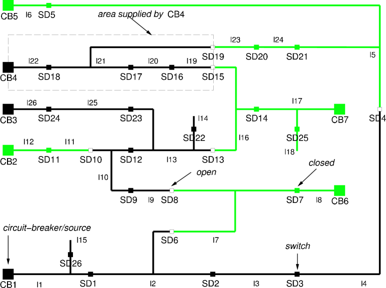
Figure 23: Sample power distribution system. Sources/circuit-breakers (e.g., CB4) are represented by large squares, and switches (e.g., SD3) by small squares. Open switches (e.g., SD8) are white. The area fed by CB4 is boxed. Gray and dark are used to distinguish adjacent areas fed by different sources

A.4.1 Application Domain

The Power Supply Restoration (PSR) domain we consider here is derived from an application investigated by Sylvie Thiébaux and others (?, ?). PSR deals with reconfiguring a faulty power distribution system to resupply customers affected by the faults. This is a topic of ongoing interest in the field of power distribution.

In more detail, a power distribution system (see Figure 23), is viewed as a network of electric lines connected by switches and fed via a number of power sources that are equipped with circuit-breakers. Switches and circuit-breakers have two possible positions, open or closed, and are connected to at most two lines. There is no restriction on the connectivity of lines, some extremities of which can also be connected to earth. When the circuit-breaker of a power source is closed, the power flows from the source to the lines downstream, until the flow is stopped by an open switch. The switches are used to appropriately configure the network and their position is initially set so that each line is fed by exactly one source.

Due to bad weather conditions, permanent faults can affect one or more lines of the network. When a power source feeds a faulty line, the circuit-breaker fitted to this source opens to protect the rest of the network from overloads. This leaves all the lines fed by the source without power. The problem consists in planning a sequence of switching operations (opening or closing switches and circuit-breakers) bringing the network into a configuration where a maximum of non-faulty lines are resupplied. For instance, suppose that line l20 becomes faulty. This leads the circuit-breaker CB4 to open and the boxed area to be without power. A possible restoration plan would be the following: open switches SD16 and SD17 to isolate the faulty line, then close SD15 to have source CB7 resupply l19, and finally re-close CB4 to resupply the others.

In the original PSR problem (?), the maximal capacity of sources and lines, as well as the load requested by customers are taken into account. The plan must optimize various numerical parameters such as breakdown costs, power margins, and distance to the initial configuration, subject to the capacity constraints. Furthermore, due to the fault sensors and switches being unreliable, the location of the faults and the current network configuration are only partially observable. When optimizing, this leads to a complex tradeoff between acting to resupply lines and acting (intrusively) to reduce uncertainty.

A.4.2 IPC-4 PDDL Adaptation

In the PDDL adaptation, we benefited from contributions by Piergiorgio Bertoli, Blai Bonet, Alessandro Cimatti, and John Slaney (?, ?). Compared to the original PSR domain described above, the IPC-4 version underwent 3 major adaptations. Firstly, the IPC deals with fully observable domains. Hence, while partial observability in PSR is a crucial issue (?, ?, ?), the IPC version assumes complete observability. Secondly, given the difficulty of encoding even the basic problem, we chose to ignore the numerical and optimization aspects of PSR (capacities, power margins, …). Thirdly, the IPC-4 version is set up as a pure goal-achievement problem, where the goal specifies a set of lines that must be (re)-supplied. We considered a more realistic goal asking the planner to supply any line that can be. However, we were unable to compile this goal into STRIPS in reasonable space, and opted for the simpler goal to keep the STRIPS formulation as consistent as possible with others.

Our highest level and most natural IPC-4 encoding of PSR involves ADL constructs and derived predicates. Briefly, the encoding works as follows. PSR problem instances specify (1) the network topology, i.e., the objects in the network and their connections (the lines, the switching devices, that is, the switches and the sources/circuit-breakers, two “side” constants side1 and side2 to denote the two connection points of a switching device, and the connection relations between those objects), (2) the initial configuration, i.e., the initial positions (open/closed) of the switching devices, and (3) the modes (faulty or not) of the various lines. Among those, only the devices’ positions can change. A number of other predicates are derived from these basic ones. They model the propagation of the current into the network with a view to determining which lines are currently fed and which sources are affected by a fault, i.e. feed a fault. The closed-world assumption semantics of PDDL2.2 derived predicates is exactly what is needed to elegantly encode such relations. These require a recursive traversal of the network paths which is naturally represented as the transitive closure of the connection relation of the network. The most complex of these derived predicates, $upstream$, requires four parameters, two of which, however can only take two possible values, and expresses that the power flows from one of the two sides of some device (side ?sx of device ?x) to one of the sides of another (side ?sy of device ?y) This happens when the side of ?x which is opposite to ?sx is directly connected to ?sy (via some line), or if there exists some closed device ?z one side of which is upstream of ?sx and the other side of which is connected to ?sy:

(:derived	(upstream ?x - DEVICE ?sx - SIDE ?y - DEVICE ?sy - SIDE)
	(and	(closed ?x)
		(or	(and (= ?sx side1) (con ?x side2 ?y ?sy))
			(and (= ?sx side2) (con ?x side1 ?y ?sy))
			(exists	(?z - DEVICE)
				(and	(closed ?z)
					(or	(and (con ?z side1 ?y ?sy) (upstream ?x ?sx ?z side2))
						(and (con ?z side2 ?y ?sy) (upstream ?x ?sx ?z side1))))))))

From upstream, it is relatively easy to define predicates stating whether a given line is fed or a given source is affected.

The goal in a problem instance asks that given lines be fed and all sources be unaffected. The available actions are closing and opening a switching device. Their effect is simply to set the device position as requested. In addition, there is an action wait, which models the event of circuit-breakers opening when they become affected. Wait is applicable when an affected source exists, and is the only applicable action in that case (the open and close actions require as a precondition that no source is affected). This, together with the goal, ensures that the wait action is applied as soon as a source is affected. The effect of the wait action is to open all the affected circuit-breakers. Concretely, the wait and close actions are as follows (note that open is similar to close and that earth is treated as a device whose position cannot be changed by the actions):

(:ac	tion close
	:parameters (?x - DEVICE)
	:precondition (and	(not (= ?x earth))
		(not (closed ?x))
		(forall (?b - DEVICE) (not (affected ?b))))
	:effect (closed ?x))
(:action wait
	:parameters ()
	:precondition (exists (?b - DEVICE) (affected ?b))
	:effect (forall (?b - DEVICE) (when (affected ?b) (not (closed ?b)))))

It would have been possible to encode the opening of affected breakers as a conditional effect of the close action. However, this would have required more complex derived predicates with an additional device as parameter and a conditional flavor, specifying, e.g., whether or not a circuit-breaker would be affected if we were to close that device.

A.4.3 IPC-4 Domain Structure

We used four domain versions of PSR in IPC-4. Primarily, these versions differ by the size of the problem instances encoded. The instance size determined in what languages we were able to formulate the domain version. We tried to generate instances of size appropriate to evaluate current planners, i.e, we scaled the instances from “push-over for everybody” to “impossibly hard for current automated planners”, where we got our intuitions by running a version of FF enhanced to deal with derived predicates. The largest instances are of the kind of size one typically encounters in the real world. More on the instance generation process is said in Section A.4.4.

The domain versions are named 1. large, 2. middle, 3. middle-compiled, and 4. small. Version 1 has the single formulation adl-derivedpredicates. Version 2 has the formulations adl-derivedpredicates, simpleadl-derivedpredicates, and strips-derivedpredicates. Version 3 has the single formulation adl, and version 4 has the single formulation strips. The formulation names simply give the language used. Version 1 contains the largest instances, versions 2 and 3 contain (the same) medium instances, and version 4 contains the smallest instances. The adl-derivedpredicates formulation is inspired by ? (?); it makes use of derived predicates as explained above, and of ADL constructs in the derived predicate, action, and goal definitions. In the simpleadl-derivedpredicates and strips-derivedpredicates formulations, all ADL constructs (except conditional effects in the simpleadl case) are compiled away. The resulting fully grounded encodings are significantly larger than the original, while on the other hand the length of plans remains nearly unaffected. The pure adl formulation is obtained from the adl-derivedpredicates formulation by compiling derived predicates away, using the method described by ? (?, ?). While there is no significant increase in the domain size, the compilation method can lead to an increase in plan length that is exponential in the arity of the derived predicates (no compilation method can avoid such a blow-up in the worst case, see ?, ?). Indeed, in our particular PSR example instances, we observed a considerable blow up in plan length. We felt that this blow up was too much to allow for a useful direct comparison of data generated for adl-derivedpredicates as opposed to adl, and we separated the adl formulation out into domain version 3 as listed above.

The strips domain formulation proved quite a challenge. All the 20 or so schemes we considered for compiling both derived predicates and ADL constructs away led to either completely unmanageable domain descriptions or completely unmanageable plans. The problem is that feasible compilations of derived predicates create new actions with highly conditional effects, and that compiling those away is impractical. We therefore adopted a different fully-grounded encoding inspired by ? (?). The encoding is generated from a description of the problem instance by a tool performing the reasoning about power propagation. In the resulting tasks, the effects of the close actions directly specify which circuit-breakers open as a result of closing a switch in a given network configuration. No derived predicates are needed, and consequently the STRIPS encoding is much simpler and only refers to the positions of the devices and not to the lines, faults, or connections. Nevertheless, we were still only able to formulate comparatively small instances in STRIPS, without a prohibitive blow-up in the encoding size.

version	formulation	$max\mbox{-}\#op$	$max\mbox{-}\#act$
large	ADL DP	7	(14038) 7498
middle	ADL DP	7	(7055) 3302
middle	SIMPLE-ADL DP	3485	(3485) 3485
middle	STRIPS DP	3560	(3560) 3560
middle-compiled	ADL	5	(99) 71
small	STRIPS	9400	(9400) 9400

Table 4: Overview over the different domain versions and formulations of PSR. Abbreviations used: “dp” derived predicates; $max\mbox{-}\#op$ is the maximum number of (parameterized) PDDL operators for any instance, $max\mbox{-}\#act$ is the maximum number of ground actions for any instance. Data in parentheses are collected before FF’s “reachability” pre-process (see text). Derivation rules (ground derivation rules) are counted as operators (ground actions).

The domain versions, formulations, and their respective numbers of operators and ground actions, are shown in Figure 4. Data in parentheses are collected before FF’s “reachability” pre-process, building a relaxed planning graph for the initial state and removing all actions that do not appear in that graph. In the encodings using ADL and derived predicates, this reduces the number of ground actions by a factor of around $2$; for only ADL, the factor is much smaller; for the other encodings, no reduction at all is obtained, simply due to the fact that these encodings are obtained with adl2strips, which uses the same pruning process. Some interesting observations can be made in the “middle” versions and formulations. The data shown there correspond to the largest instance that FF’s pre-processor could handle in all versions/formulations, to enable direct comparison. We see that, for formulation in SIMPLE-ADL and STRIPS, we need to introduce some more ground actions. We also see that, curiously, in the compilation of derived predicates (compilation to “middle-compiled”), the number of ground actions decreases dramatically. The reason for this lies in that these data count ground derivation rules as ground actions, and in the subtleties of the compilation of derived predicates. In the “middle” formulations, almost all ground actions are in fact ground derivation rules. These are compiled away for “middle-compiled” following ? (?, ?), introducing a single action that has one distinct conditional effect for each derivation rule, c.f. Section 2. Which just means that the complexity of thousands of derivation rules is replaced with the complexity of an action with thousands of conditional effects.

A.4.4 IPC-4 Example Instances

Due to contractual agreements, we were unable to use real data in the competition. Instead, PSR instances were randomly generated using “randomnet”, a special purpose tool implemented by John Slaney.

Power distribution networks often have a mesh-able structure exploited radially: the path taken by the power of each source forms a tree whose nodes are switches and whose arcs are electric lines; terminal switches connect the various trees together. Randomnet takes as input the number of sources, a percentage of faulty lines, and a range of parameters for controlling tree depth, branching, and tree adjacency, whose default values are representative of real networks. Randomnet randomly generates a network topology and a set of faulty lines. These are turned into the various PDDL encodings above by a tool called net2pddl, implemented by Piergiorgio Bertoli and Sylvie Thiébaux. net2pddl computes the set of all lines that can be supplied, and makes this the goal.

The instances we generated make use of randomnet default settings, with two exceptions to create problems of increasing difficulty. The first is that the maximal depth of the trees takes a range of values up to twice the default. The larger this value, the harder the problem. The second is that the percentage of faulty lines ranges from 0.1 to 0.7. Problems at the middle of the range are harder on average, those at the bottom of the range are more realistic.

Each instance suite contains 50 instances. The small instances feature between 1 to 6 sources, the middle instances feature up to 10 sources, and the large instances feature up to 100 sources. The large instances are of a size typical for real-world instances, or even larger. The example in Figure 23 is representative of a difficult instance in the middle set.

A.4.5 Future Work

While PSR has been around for some time as a benchmark for planning under uncertainty, we expect that the work done in the framework of IPC-4 will facilitate its acceptance as one of the standard benchmarks for planning. To this end, we have developed a PSR resource web page giving access to the relevant papers, data, and tools (net2pddl, randomnet, …). One aspect of future work is to complete and maintain this website, making available a number of already existing tools, such as SyDRe (?), a domain-specific system for the full PSR problem, and Matt Gray’s net2jpeg which graphically displays networks generated by randomnet.

Considering future IPCs, there is potential for extending the PDDL encoding to take the numerical and optimization aspects of the benchmark into account. PDDL-like encodings of the partially observable version of the benchmark exist (?) and are ready to be used in a future edition of the probabilistic part of the IPC.

A.5 Satellite

The Satellite domain was introduced in IPC-3 by ? (?). It is motivated by a NASA space application: a number of satellites have to take images of a number of spatial phenomena, obeying constraints such as data storage space and fuel usage. In IPC-3, there were 5 versions of the domain, corresponding to different levels of the language PDDL2.1: Strips, Numeric, SimpleTime (action durations are constants), Time (action durations are expressions in static variables), and Complex (durations and numerics, i.e. the “union” of Numeric and Time).

The adaptation of the Satellite domain for IPC-4 was done by Jörg Hoffmann. All IPC-3 domain versions and example instances were re-used, except SimpleTime – like in the other IPC-4 domains, we didn’t want to introduce an extra version distinction just for the difference between constant durations and static durations. On top of the IPC-3 versions, 4 new domain versions were added. The idea was to make the domain more realistic by additionally introducing time windows for the sending of the image data to earth, i.e. to antennas that are visible for satellites only during certain periods of time – according to Derek Long, the lack of such time windows was the main shortcoming of the IPC-3 domain.

We extended the IPC-3 Time domain version to two IPC-4 domain versions, Time-timewindows and Time-timewindows-compiled. We extended the IPC-3 Complex domain version to the two IPC-4 domain versions Complex-timewindows and Complex-timewindows-compiled. In all cases, we introduced a new action for the sending of data to an antenna. An antenna can receive data of only a single satellite at a time, an antenna is visible for only subsets of the satellites for certain time periods, and the sending of an image takes time proportional to the size of the image. The time windows were modelled using timed initial literals, and in the “-compiled” domain versions, these literals were compiled into artificial PDDL constructs. None of the domain versions uses ADL constructs, so of all versions there is only a single (STRIPS) formulation.

The instances were generated as follows. Our objectives were to clearly demonstrate the effect of additional time windows, and to produce solvable instances only. To accomplish the former, we re-used the IPC-3 instances, so that the only difference between, e.g., Time and Time-timewindows, lies in the additional time window constructs. To ensure solvability, we implemented a tool that read the plans produced by one of the IPC-3 participants, namely TLPlan, and then arranged the time windows so that the input plan was suitable to solve the enriched instance. It is important to note here that the time windows were not arranged to exactly meet the times extracted from the IPC-3 plan. Rather, we introduced one time window per each 5 “take-image” actions, made the antenna visible during that time window for only the respective 5 satellites, and let the image size for each individual image be a random value within a certain range where the time window was 5 times as long as the sending time resulting from the maximum possible size.

Of course, the above generation process is arranged rather arbitrarily, and the resulting instances might be a long way away from the typical characteristics of the Satellite problem as it occurs in the real world. While this isn’t nice, it is the best we could do without inside knowledge of the application domain, and it has the advantage that the enriched instances are solvable, and directly comparable to the IPC-3 ones.

In the new domain versions derived from Complex, we also introduced utilities for the time window inside which an image is sent to earth. For each image, the utility is either the same for all windows, or it decreases monotonically with the start time of the window, or it is random within a certain interval. Each image was put randomly into one of these classes, and the optimization requirement is to minimize a linear combination of makespan, fuel usage, and summed up negated image utility.

A.6 Settlers

The Settlers domain was introduced in IPC-3 by ? (?). It makes extensive use of numeric variables. These variables carry most of the domain semantics, which is about building up an infrastructure in an unsettled area, involving the building of housing, railway tracks, sawmills, etc. The domain was included into IPC-4 in order to pose a challenge for the numeric planners – the other domains mostly do not make much use of numeric variables, other than computing the (static) durations of actions. We used the exact same domain file and example instances as in IPC-3, except that we removed some universally quantified preconditions to improve accessibility for planners. The quantifiers ranged over domain constants only so they could easily be replaced by conjunctions of atoms.

A.7 UMTS

Roman Englert has been working in this application area for several years. The domain was adapted for IPC-4 by Stefan Edelkamp and Roman Englert.

A.7.1 Application Domain

Probably the best known feature of UMTS (Universal Mobile Telecommunication Standard) is higher bit rate (?): packet-switched connections can reach up to 2 mega bit per second (Mbps) in the optimal case. Compared to existing mobile networks, UMTS provides a new and important feature, namely the negotiation of Quality of Service (QoS) and of transfer properties. The attributes that define the characteristics of the transfer are throughput, transfer delay, and data error rate. UMTS bearers have to be generic in order to provide good support for existing applications and the evolution of new applications. Applications and services are divided into four traffic classes by their QoS (?, ?). The traffic classes, their fundamental characteristics, and examples for applications are summarized in Table 5.

Class	Conversational	Streaming	Interactive	Background
	Preserve time	Preserve time	Request res-	Undefined
	relation between	relation between	ponse pattern.	delay.
Constraints	information flow	information	Preserve data	Preserve
	on the stream.	entities of the	integrity	data
	Conversational	stream		integrity
	pattern (low delay)
	Voice, video	Streaming	Web browsing,	Background
Examples	telephony &	multimedia	network games	download
	video games			of e-mails

Table 5: UMTS quality of service classes and their characteristics.

The main distinguishing factor between these classes is how delay-sensitive the traffic is: the conversational class is very delay sensitive (approximately 40 ms time preservation), and the background class has no defined maximum delay.

The UMTS call set-up can be modularized using the perspective of Intelligent Software Agents (?, ?), since agents are logical units and enable a discrete perspective of the continuous signaling process. The call set-up is partitioned into the following modules that are executed in sequential order (?):

TRM

The initial step is the initiation of an application on the mobile and the determination of the required resources for the execution. The resources of the mobile like display and memory are checked by the Terminal Resource Management (TRM) and allocated, if possible. Otherwise, the execution is aborted.

CT

The wireless connection to the radio network is initiated via the dedicated control channel of GSM (?). In case of success, the transmission of ”Ready for service” is transferred via the node B to the mobile in order to ensure the Connection Timing (CT) for bearer service availability.

AM

The information of the mobile like location and data handling capabilities is sent to the application server in the Internet (cf. AEEI). The transmission can be done comfortably by a so-called service agent (?) that is controlled by the Agent Management (AM) in the CND. The advantage of a service agent is, that in case of failure, e.g., network resources are not sufficiently available, the agent can negotiate with the terminal’s agent about another QoS class or different quality parameters.

AEEM

A service agent with the required QoS class for the execution of the application and with parameters of the mobile application is sent from the mobile’s Agent Execution Environment Mobile (AEEM) to the application server in the Internet (cf. AEEI).

RRC

The Radio Resource Controller (RRC) provisions/allocates the required QoS by logical resources from the MAC level in the radio bearer (?).

RAB

Then, the bearer resources are supplied on the physical level from the Radio Access Bearer (RAB) from the CND and the call flow is set-up by mapping the logical QoS parameters and the physical QoS resources together.

AEEI

The Agent Execution Environment Internet (AEEI) establishes the data transfer from the core network to a PDN (e.g., Internet) and sends a service agent (controlled by AM) to the application in the PDN in order to ensure the QoS for the application.

BS

Finally, the Bearer Service (BS) for the execution of the mobile application is established with the required radio bearer resources with QoS. Messages are sent to the modules TRM and AEEI to start the execution of the application.

These modules are executed in sequential order to set-up a call for the execution of mobile applications. Two modules (AEEM and AEEI) have to be executed in time windows in order to ensure that the agents are life in the network. However, two constraints have been added: First, the intra-application constraint, where modules from one application are ordered. Second, the inter-application constraint, where modules with same names from different applications cannot be executed in parallel in order to ensure that the required resources are available.

A.7.2 IPC-4 PDDL Adaptation

Besides action duration, the domain encodes scheduling types of resources, consuming some amount at action initialization time and releasing the same amount at action ending time. Scheduling types of resources have not been used in planning benchmarks before, and the good news is that temporal PDDL2.1 (Level 3) is capable of expressing them. In fact we used a similar encoding to the one that we found for Job- and Flow-Shop problems. As one feature, actions are defined to temporarily produce rather than to temporarily consume resources. As current PDDL has no way of stating such resource constraints explicitly, planners that want to exploit that knowledge have to look for a certain patterns of increase/decrease effects to recognize them. Additionally, the resource modeling of our UMTS adaptation is constrained to the most important parameters (in total 15). In real networks several hundred parameters are applied.

In UMTS, two subsequent actions can both check and update the value of some resources (e.g., has-mobile-cpu) at their starting (resp. ending) time points as far as the start (resp. ending) events are separated by $\epsilon$ time steps, where $\epsilon$ is minimum slack time required between two dependent events. When modeling renewable resources with an over all construct the invariant condition of the action has to check, what the at start event did change. We decided that this is not the best choice for a proper temporal action. Consequently, the temporal actions require resources to be available before adding the amount used.

Finally, the time windows for the two agent-based modules are defined using the average execution times of the modules. The average times are estimated based on signaling durations of the UMTS network (?).

mobile-cpu	used with $x$ per cent per application
d-available	partition of the display, e.g., ticker and chess
e-balance	energy balance of mobile accumulator
mobile-channels	used for data transfer
-available
num-mobiles	number of mobiles which are tractable
	by a node B
num-calls	mobile network load for a node B
mobile-storage	memory on S(IM)AT card
logical-channels	number of logical channels available in the CN
cell-update	report UE location into RNC
handover	handover required to get a higher bit rate
active-set-up	update connection
ggsn-bitrate	capacity (kbit/s) from GGSN to PDN
max-no-pdp	max. no. of packet data protocols per mobile
max-no-apn	max. access point names (APN) per mobile

Table 6: Scheduling types of resources in the UMTS call set-up.

Resources may be renewable or consumable: an example for a renewable resource is the keyboard of the mobile. It can be used to input data for several applications. Consumable resources are released after action execution. The resources that are realized in the experiments are summarized in Table 6 (see ? for a complete list of resources for the UMTS call set-up).

The PDDL representation of the planning domain is based on the eight modules for the UMTS call set-up. There are eight operators corresponding to these eight modules. Let us consider, as an example, the BS action, that is, the final action that can be used to establish the predicate bs-ok. It is defined as follows:

(	:durative-action BS
	:parameters
	(?A-new - application ?M - mobile ?L - list ?MS1 ?MS2 - message ?a - agent)
	:duration
	(= ?duration (time-bs ?A-new))
	:condition
	(and	(at start (initiated ?A-new ?M))
		(at start (aeei-ok ?A-new ?M ?L ?a))
		(at start (qos-params ?A-new ?L))
		(at start (message-trm ?M ?MS1))
		(at start (message-aeei ?A-new ?MS2)))
	:effect
	(and (at end (iu-bearer ?A-new ?M ?L)) (at end (bs-ok ?A-new ?M ?L ?a)))))

The action has as preconditions the successful execution of the module AEEI during the call set-up, the satisfaction of the required QoS class parameters (denoted as list $L$), and the transfered messages of the set-up status to the application in the mobile and the PDN. The resources are already allocated by the preceding modules. As effect the bearer and the network connection for the mobile application are set up.

The initiation of an application starts in the mobile with the TRM. Afterwards, the CT in the AND is asked for a ready-for-service signal. In the core of the call set-up is the radio access bearer procedure in the CND. Let us consider the latter in more detail. As first step the logical resources must be allocated (RRC), e.g., the required number of channels must be provided by the logical level in the radio bearer and later these logical resources are mapped to the physical channels. The PDDL RRC action looks as follows:

(	:durative-action RRC
	:parameters
	(?A-new - application ?M - mobile ?L - list ?a - agent)
	:duration
	(= ?duration (time-rrc ?A-new))
	:condition
	(and	(at start (ct-ok ?A-new ?M ?L))
		(at start (aeem-ok ?A-new ?M ?L ?a))
		(at start ($<$=	(has-logical-channels)
			(- (max-logical-channels) (app-channels ?A-new ?m))))
		(at start ($<$= (has-cell-update) (- (max-cell-update) 2)))
		(at start ($<$ (has-handover) (max-handover)))
		(at start ($<$ (has-active-set-up) (max-active-set-up))))
	:effect
	(and	(at start (increase (has-logical-channels) (app-channels ?A-new ?M)))
		(at end (decrease (has-logical-channels) (app-channels ?A-new ?M)))
		(at start (increase (has-cell-update) 2))
		(at end (decrease (has-cell-update) 2))
		(at start (increase (has-handover) 1))
		(at end (decrease (has-handover) 1))
		(at start (increase (has-active-set-up) 1))
		(at end (decrease (has-active-set-up) 1))
		(at end (rrc-ok ?A-new ?M ?L ?a))))

If the requested QoS class is not available, then the fact rab-ok is not true and a service agent must be sent to the mobile in order to negotiate with the application or user for weaker QoS requirements. In case of success the predicate rab-ok is true and the connection to the PDN must be checked. Finally, the goal predicate BS can be fulfilled if all resources are available.

A.7.3 IPC-4 Domain Structure

As used in IPC-4, the UMTS domain has six versions. The first three are: temporal, a domain version with no timing constraints, temporal-timewindows, a domain version with PDDL2.2 timed initial facts, and temporal-timewindows-compiled, a domain version with a PDDL2.1 wrapper encoding for the timed initial literals. The second domain version set flaw-temporal, flaw-temporal-timewindows, and flaw-temporal-timewindows-compiled, includes the following “flaw” action:

(	:durative-action FLAW
	parameters
	(?A-new - application ?M - mobile ?L - list ?a - agent)
	:duration (= ?duration 4)
	:condition
	(and	(at start (initiated ?A-new ?M))
		(at start (qos-params ?A-new ?L))
		(at start (trm-ok ?A-new ?M ?L)))
	:effect
	(and	(at end (rab-ok ?A-new ?M ?L ?a))
		(at start (not (initiated ?A-new ?M)))))

This action offers a shortcut to the rab-ok predicate, but can not be used in a real solution because it deletes the initiated predicate. But the action can be used in heuristic functions based on ignoring the negative effects. In that sense, the action encodes a flaw that may disturb the heuristic techniques used in modern planners. To determine that the action is not useful, negative interactions have to be considered. The idea of flaw is practically motivated in order to see how heuristic planners react to it. In its standard form, the domain is not a big challenge to such planners, as we have seen in Section 5. All domain versions have one formulation, namely strips-fluents-temporal, where numerical fluents, but - except typing - no ADL constructs are used. In all instances, the plan objective is to minimize makespan.

version	formulation	$max\mbox{-}\#op$	$max\mbox{-}\#act$
temporal	STRIPS-TEMPORAL	8	(5120) 80
temporal-tw	STRIPS-TEMPORAL-TW	8	(5120) 80
temporal-twc	STRIPS-TEMPORAL	13	(5125) 85
flaw-temporal	STRIPS-TEMPORAL	9	(5310) 90
flaw-temporal-tw	STRIPS-TEMPORAL-TW	9	(5310) 90
flaw-temporal-twc	STRIPS-TEMPORAL	14	(5315) 95

Table 7: Overview over the different domain versions of UMTS. Abbreviations used: “temporal-tw” for “temporal-timewindows”, “temporal-twc” for temporal-timewindows-compiled; $max\mbox{-}\#op$ is the maximum number of (parameterized) PDDL operators for any instance, $max\mbox{-}\#act$ is the maximum number of ground actions for any instance. Data in parentheses are collected before FF’s “reachability” pre-process (see text).

The domain versions and numbers of operators and ground actions are overviewed in Table 7. As with many of the empirical data for UMTS that we have seen before, the data are quite exceptional, and at the same time easy to interpret. First, similar to what we have seen in Section 5.3, the data are actually constant across all instances within each domain version, which is once again due to the fact that the instances scale only in their specification of what applications need actually be started. Second, the numbers of operators and actions do not differ between the versions with and without time windows; they increase somewhat, through the additional artificial actions, if we compile timed initial literals away (c.f. Section 2); they also increase somewhat, of course, if we introduce the “flaw” action. Third, the most striking observation is the huge effect of FF’s reachability pre-processor, building a relaxed planning graph for the initial state and removing all actions that do not appear in that graph. This is due to the technical subtleties of the encoding, where the restrictions on feasible action instantiations are, partly, implicit in the possible action sequences, rather than explicit in the static predicates.

A.7.4 IPC-4 Example Instances

The UMTS call set-up domain has the following challenges for the planning task (?):

Real-time:

Can plans for the execution of mobile applications be generated in an appropriate time? Planning has to be done with a maximum duration that does not exceed the UMTS call set-up time.

Completeness:

Is it possible to generate the plan, i.e. does planning result in an (optimal) plan for the required applications that minimizes the waiting period until all applications are started?

The PDDL structure of the basic problem for the discrete UMTS call set-up (DUCS) domain is the following:

(define (problem DUCS DOMAIN BASIC VERSION)
(:domain DUCS_DOMAIN_BASIC_VERSION
(:objects	MS1 MS2 - message
	A1 A2 A3 A4 A5 A6 A7 A8 A9 A10 - application
	M1 M2 M3 M4 M5 M6 M7 M8 M9 M10 - mobile
	L1 L2 L3 L4 L5 L6 L7 L8 L9 L10 - list
	ae - agent)
(:init	(= (time-trm A1) 76) (= (time-ct A1) 48)
	(= (time-am A1) 74) (= (time-aeem A1) 66)
	(= (time-rrc A1) 202) (= (time-rab A1) 67)
	(= (time-aeei A1) 36) (= (time-bs A1) 28)
	[…]
	(location M1) ;; types
	(authentification M1)
	[…]
	(= (has-mobile-cpu) 0) ;; current status
	[…] )
(:goal (and (bs-ok A1 M1 L1 ae) […] )))

First in this PDDL description come the objects for the applications and the mobiles. Then come the durations of the modules depending on the applications, e.g., the module TRM requires less time for a news ticker than for a chess game, since the latter requires more terminal resources than the ticker. The current status of the resources is initialized. Finally, the goal is defined: the bearer establishment for the execution start of the initiated mobile applications. The total execution time should be minimized.

For IPC-4 the time windows are varied with small perturbations in order to generate different instances. The perturbations are motivated by the average execution times of the modules in a radio network according to the load. Furthermore, the number of applications to be set up is varied from 1 up to 10. The domains assume that the applications run on one mobile terminal. However, they can also be distributed to several mobile terminals. There are 50 different instances per domain version.

A.7.5 Future Work

The UMTS domain is not a big challenge for modern heuristic, i.e. HSP/FF/LPG-style, planners because these planners are satisficing (potentially return sub-optimal plans). The objective in UMTS is to minimize the execution time, and if one ignores that objective then the task trivializes. To the optimal planners, UMTS is a realistic challenge. The domain is already relatively realistically modelled, except for the left-out additional constraints on the (many) less important resources. It remains to be seen if, when introducing all these resources, planner (in particular optimal planner) performance gets degraded. An option in this case may be to introduce explicit language constructs for the different types (renewable and consumable) of resources.

In the future the following two challenges shall be investigated. First, the negotiation of UMTS Quality of Service (QoS) parameters could be considered. Assume a video application on a mobile terminal is initiated, but the bearer resources are not sufficiently available. Then the QoS has to be negotiated between the terminal and the bearer. This leads to the planning of a negotiation during the plan execution for the already initiated applications.

Second, the approach for the optimization of the UMTS call set-up can be applied to the Wireless LAN registration. The challenge is to transfer the QoS parameters, since the current Wireless LAN standard (802.11b) does not contain QoS. This demerit can be solved by applying an additional service level that addresses QoS.

References

- 3GPP 3GPP (2004). 3G Partnership Project, www.3gpp.org.
- Appleby and Steward Appleby, S., and Steward, T. (1999). Mobile Software Agents for Control in Telecommunication Networks, chap. 11 in Hayzelden, A./Bigham, J. (eds.), Software Agents for Future Telecommunication Systems. Springer.
- Apt et al. Apt, K., Blair, H., and Walker, A. (1988). Towards a theory of declarative knowledge. In Foundations of Deductive Databases and Logic Programming, pp. 89–148. Morgan Kaufmann.
- Bacchus and Kabanza Bacchus, F., and Kabanza, F. (2000). Using temporal logics to express search control knowledge for planning. Artificial Intelligence, 116, 123–191.
- Bacchus Bacchus, F. (2000). Subset of PDDL for the AIPS2000 Planning Competition. The AIPS-00 Planning Competition Comitee. Available at http://www.cs.toronto.edu/aips2000/pddl-subset.ps.
- Bacchus Bacchus, F. (2001). The AIPS’00 planning competition. The AI Magazine, 22(3), 47–56.
- Bertoli et al. Bertoli, P., Cimatti, A., Roveri, M., and Traverso, P. (2001). Planning in nondeterministic domains under partial observability via symbolic model checking.. In Nebel (?).
- Bertoli et al. Bertoli, P., Cimatti, A., Slaney, J., and Thiébaux, S. (2002). Solving power supply restoration problems with planning via symbolic model checking. In Proceedings of the 15th European Conference on Artificial Intelligence (ECAI-02), pp. 576–80, Lyon, France. Wiley.
- Biundo et al. Biundo, S., Myers, K., and Rajan, K. (Eds.)., ICAPS-05 (2005). Proceedings of the 15th International Conference on Automated Planning and Scheduling (ICAPS-05), Monterey, CA, USA. Morgan Kaufmann.
- Bloem et al. Bloem, R., Ravi, K., and Somenzi, F. (2000). Symbolic guided search for CTL model checking. In Conference on Design Automation (DAC), pp. 29–34.
- Blum and Furst Blum, A. L., and Furst, M. L. (1997). Fast planning through planning graph analysis. Artificial Intelligence, 90(1-2), 279–298.
- Boddy et al. Boddy, M., Gohde, J., Haigh, T., and Harp, S. (2005). Course of action generation for cyber security using classical planning.. In Biundo et al. (?), pp. 12–21.
- Bonet and Geffner Bonet, B., and Geffner, H. (2001). Planning as heuristic search. Artificial Intelligence, 129(1–2), 5–33.
- Bonet et al. Bonet, B., Loerincs, G., and Geffner, H. (1997). A robust and fast action selection mechanism for planning. In Proceedings of the 14th National Conference of the American Association for Artificial Intelligence (AAAI-97), pp. 714–719. MIT Press.
- Bonet and Thiébaux Bonet, B., and Thiébaux, S. (2003). GPT meets PSR. In Giunchiglia, E., Muscettola, N., and Nau, D. (Eds.), Proceedings of the 13th International Conference on Automated Planning and Scheduling (ICAPS-03), pp. 102–111, Trento, Italy. Morgan Kaufmann.
- Busuioc Busuioc, M. (1999). Distributed Intelligent Agents - A Solution for the Management of Complex Telecommunications Services, chap. 4 in Hayzelden, A./Bigham, J. (eds.), Software Agents for Future Telecommunication Systems. Springer.
- Bylander Bylander, T. (1994). The computational complexity of propositional STRIPS planning. Artificial Intelligence, 69(1–2), 165–204.
- Cesta and Borrajo Cesta, A., and Borrajo, D. (Eds.). (2001). Recent Advances in AI Planning. 6th European Conference on Planning (ECP’01), Toledo, Spain. Springer-Verlag.
- Chen et al. Chen, Y., Hsu, C., and Wah, B. (2004). SGPlan: Subgoal partitioning and resolution in planning. In Edelkamp, S., Hoffmann, J., Littman, M., and Younes, H. (Eds.), Proceedings of the 4th International Planning Competition, Whistler, BC, Canada. JPL.
- Chien et al. Chien, S., Kambhampati, R., and Knoblock, C. (Eds.)., AIPS-00 (2000). Proceedings of the 5th International Conference on Artificial Intelligence Planning Systems (AIPS-00). AAAI Press, Menlo Park.
- Cimatti et al. Cimatti, A., Roveri, M., and Traverso, P. (1998). Automatic OBDD-based generation of universal plans in non-deterministic domains. In Proceedings of the 15th National Conference of the American Association for Artificial Intelligence (AAAI-98), pp. 875–881, Madison, WI. MIT Press.
- Clarke et al. Clarke, E. M., Grumberg, O., and Peled, D. A. (1999). Model Checking. MIT Press.
- Dierks Dierks, H. (2005). Finding optimal plans for domains with restricted continuous effects with uppaal cora. In ICAPS Workshop on Verification and Validation of Model-Based Planning and Scheduling Systems.
- Edelkamp Edelkamp, S. (2003a). Promela planning. In Workshop on Model Checking Software (SPIN), Lecture Notes in Computer Science, pp. 197–212. Springer.
- Edelkamp Edelkamp, S. (2003b). Taming numbers and durations in the model checking integrated planning system. Journal of Artificial Intelligence Research, 20, 195–238.
- Edelkamp and Jabbar Edelkamp, S., and Jabbar, S. (2005). Action planning for directed model checking of Petri nets. Electronic Notes in Theoretical Computer Science, 149(2), 3–18.
- Edelkamp et al. Edelkamp, S., Jabbar, S., and Lluch-Lafuente, A. (2005). Action planning for graph transition systems. In ICAPS Workshop on Verification and Validation of Model-Based Planning and Scheduling Systems, pp. 48–57.
- Edelkamp et al. Edelkamp, S., Leue, S., and Lluch-Lafuente, A. (2004). Directed explicit-state model checking in the validation of communication protocols. International Journal on Software Tools for Technology, 5, 247 – 267.
- Englert Englert, R. (2005). Planning to optimize the UMTS call set-up for the execution of mobile applications. Int. Journal of Applied Artificial Intelligence, 19(2), 99–117.
- Englert and Cremers Englert, R., and Cremers, A. B. (2001). Configuration of Applications for the 3rd Generation Mobile Communication. In KI Workshop on AI in Planning, Scheduling, Configuration and Design (PUK). Vienna, Austria.
- Farjami et al. Farjami, P., Görg, C., and Bell, F. (2000). Advanced service provisioning based on mobile agents. Computer Communications, 23, 754 – 760.
- Fikes and Nilsson Fikes, R. E., and Nilsson, N. (1971). STRIPS: A new approach to the application of theorem proving to problem solving. Artificial Intelligence, 2, 189–208.
- Fourman Fourman, M. P. (2000). Propositional planning. In AIPS Workshop on Model-Theoretic Approaches to Planning.
- Fox et al. Fox, M., Long, D., and Halsey, K. (2004). An investigation into the expressive power of PDDL2.1. In Saitta, L. (Ed.), Proceedings of the 16th European Conference on Artificial Intelligence (ECAI-04), Valencia, Spain. Wiley.
- Fox and Long Fox, M., and Long, D. (1999). The detection and exploitation of symmetry in planning problems. In Pollack, M. (Ed.), Proceedings of the 16th International Joint Conference on Artificial Intelligence (IJCAI-99), pp. 956–961, Stockholm, Sweden. Morgan Kaufmann.
- Fox and Long Fox, M., and Long, D. (2003). PDDL2.1: An extension to PDDL for expressing temporal planning domains. Journal of Artificial Intelligence Research, 20, 61–124.
- Frank et al. Frank, J., Cheeseman, P., and Stutz, J. (1997). When gravity fails: Local search topology. Journal of Artificial Intelligence Research, 7, 249–281.
- Garagnani Garagnani, M. (2000). A correct algorithm for efficient planning with preprocessed domain axioms. In Research and Development in Intelligent Systems XVII. Springer-Verlag.
- Gazen and Knoblock Gazen, B. C., and Knoblock, C. (1997). Combining the expressiveness of UCPOP with the efficiency of Graphplan.. In Steel, and Alami (?), pp. 221–233.
- Gerevini and Long Gerevini, A., and Long, D. (2005). Plan Constraints and Preferences. The AIPS-06 Planning Competition Comitee. Available at http://zeus.ing.unibs.it/ipc-5/pddl-ipc5.pdf.
- Gerevini et al. Gerevini, A., Saetti, A., and Serina, I. (2006). An approach to temporal planning and scheduling in domains with predictable exogenous events. Journal of Artificial Intelligence Research, 25, 187–231.
- Giunchiglia and Traverso Giunchiglia, F., and Traverso, P. (1999). Planning as model checking. In Biundo, S., and Fox, M. (Eds.), Recent Advances in AI Planning. 5th European Conference on Planning (ECP’99), Lecture Notes in Artificial Intelligence, pp. 1–19, Durham, UK. Springer-Verlag.
- Haslum and Geffner Haslum, P., and Geffner, H. (2001). Heuristic planning with time and resources.. In Cesta, and Borrajo (?), pp. 121–132.
- Hatzack Hatzack, W. (2002). Entwicklung und Auswertung von Algorithmen zur autonomen Verkehrskoordinierung und Konfliktaufl sung an Flugh fen. Ph.D. thesis, University of Freiburg, Freiburg, Germany.
- Hatzack and Nebel Hatzack, W., and Nebel, B. (2001). The operational traffic control problem: Computational complexity and solutions.. In Cesta, and Borrajo (?), pp. 49–60.
- Helmert Helmert, M. (2003). Complexity results for standard benchmark domains in planning. Artificial Intelligence, 143, 219–262.
- Helmert Helmert, M. (2004). A planning heuristic based on causal graph analysis.. In Koenig et al. (?), pp. 161–170.
- Helmert Helmert, M. (2005) Personal communication.
- Helmert Helmert, M. (2006a). The fast downward planning system. Journal of Artificial Intelligence Research, 26. Accepted for Publication.
- Helmert Helmert, M. (2006b). New complexity results for classical planning benchmarks. In Long, D., and Smith, S. (Eds.), Proceedings of the 16th International Conference on Automated Planning and Scheduling (ICAPS-06), pp. 52–61, The English Lake District, UK. Morgan Kaufmann.
- Hoffmann Hoffmann, J. (2001). Local search topology in planning benchmarks: An empirical analysis.. In Nebel (?), pp. 453–458.
- Hoffmann Hoffmann, J. (2002). Local search topology in planning benchmarks: A theoretical analysis. In Ghallab, M., Hertzberg, J., and Traverso, P. (Eds.), Proceedings of the 6th International Conference on Artificial Intelligence Planning and Scheduling (AIPS-02), pp. 92–100, Toulouse, France. Morgan Kaufmann.
- Hoffmann Hoffmann, J. (2003). The Metric-FF planning system: Translating “ignoring delete lists” to numeric state variables. Journal of Artificial Intelligence Research, 20, 291–341.
- Hoffmann Hoffmann, J. (2005). Where ‘ignoring delete lists’ works: Local search topology in planning benchmarks. Journal of Artificial Intelligence Research, 24, 685–758.
- Hoffmann and Edelkamp Hoffmann, J., and Edelkamp, S. (2005). The deterministic part of IPC-4: An overview. Journal of Artificial Intelligence Research, 24, 519–579.
- Hoffmann and Nebel Hoffmann, J., and Nebel, B. (2001). The FF planning system: Fast plan generation through heuristic search. Journal of Artificial Intelligence Research, 14, 253–302.
- Hölldobler and Stör Hölldobler, S., and Stör, H.-P. (2000). Solving the entailment problem in the fluent calculus using binary decision diagrams. In ICAPS Workshop on Model-Theoretic Approaches to Planning.
- Holma and Toskala Holma, H., and Toskala, A. (2000). WCDMA for UMTS - Radio Access for 3rd Generation Mobile Communications. Wiley & Sons.
- Holzmann Holzmann, G. (2003). The Spin Model Checker - Primer and Reference Manual. Addison-Wesley.
- Holzmann Holzmann, G. J. (1990). Design and Validation of Computer Protocols. Prentice Hall.
- Howe and Dahlman Howe, A., and Dahlman, E. (2002). A critical assessment of benchmark comparison in planning. Journal of Artificial Intelligence Research, 17, 1–33.
- Kabanza and Thiébaux Kabanza, F., and Thiébaux, S. (2005). Search control in planning for temporally extended goals.. In Biundo et al. (?), pp. 130–139.
- Koehler and Hoffmann Koehler, J., and Hoffmann, J. (2000). On the instantiation of ADL operators involving arbitrary first-order formulas. In ECAI Workshop on New Results in Planning, Scheduling and Design.
- Koehler, Nebel, Hoffmann, and Dimopoulos Koehler, J., Nebel, B., Hoffmann, J., and Dimopoulos, Y. (1997). Extending planning graphs to an ADL subset.. In Steel, and Alami (?), pp. 273–285.
- Koehler and Schuster Koehler, J., and Schuster, K. (2000). Elevator control as a planning problem.. In Chien et al. (?), pp. 331–338.
- Koenig, Zilberstein, and Koehler Koenig, S., Zilberstein, S., and Koehler, J. (Eds.)., ICAPS-04 (2004). Proceedings of the 14th International Conference on Automated Planning and Scheduling (ICAPS-04), Whistler, Canada. Morgan Kaufmann.
- Korf Korf, R. E. (1990). Real-time heuristic search. Artificial Intelligence, 42, 189–211.
- Kvarnström, Doherty, and Haslum Kvarnström, J., Doherty, P., and Haslum, P. (2000). Extending TALplanner with concurrency and ressources. In Horn, W. (Ed.), Proceedings of the 14th European Conference on Artificial Intelligence (ECAI-00), pp. 501–505, Berlin, Germany. Wiley.
- Lago, Pistore, and Traverso Lago, U. D., Pistore, M., and Traverso, P. (2002). Planning with a language for extended goals. In Proceedings of the 18th National Conference of the American Association for Artificial Intelligence (AAAI-02), pp. 447–454, Edmonton, AL. MIT Press.
- Long and Fox Long, D., and Fox, M. (2000). Automatic synthesis and use of generic types in planning.. In Chien et al. (?), pp. 196–205.
- Long and Fox Long, D., and Fox, M. (2003). The 3rd international planning competition: Results and analysis. Journal of Artificial Intelligence Research, 20, 1–59.
- McDermott McDermott, D. (1996). A heuristic estimator for means-ends analysis in planning. In Proceedings of the 3rd International Conference on Artificial Intelligence Planning Systems (AIPS-96), pp. 142–149. AAAI Press, Menlo Park.
- McDermott McDermott, D. (1998). The PDDL Planning Domain Definition Language. The AIPS-98 Planning Competition Comitee. Available at http://ls5-www.cs.uni-dortmund.de/ edelkamp/ipc-4/DOCS/pddl.ps.gz.
- McDermott McDermott, D. (2000). The 1998 AI planning systems competition. The AI Magazine, 21(2), 35–55.
- McDermott McDermott, D. V. (1999). Using regression-match graphs to control search in planning. Artificial Intelligence, 109(1-2), 111–159.
- Milidiú and dos Santos Liporace Milidiú, R. L., and dos Santos Liporace, F. (2004a). Plumber, a pipeline transportation planner. In International Workshop on Harbour and Maritime Simulation (HMS), pp. 99–106, Rio de Janeiro, Brazil.
- Milidiú and dos Santos Liporace Milidiú, R. L., and dos Santos Liporace, F. (2004b). Pipesworld: Applying planning systems to pipeline transportation. In Proceedings of the International Pipeline Conference (IPC), pp. 713–719.
- Nebel Nebel, B. (Ed.)., IJCAI-01 (2001). Proceedings of the 17th International Joint Conference on Artificial Intelligence (IJCAI-01), Seattle, Washington, USA. Morgan Kaufmann.
- Nebel Nebel, B. (2000). On the compilability and expressive power of propositional planning formalisms. Journal of Artificial Intelligence Research, 12, 271–315.
- Pednault Pednault, E. P. (1989). ADL: Exploring the middle ground between STRIPS and the situation calculus. In Brachman, R., Levesque, H. J., and Reiter, R. (Eds.), Principles of Knowledge Representation and Reasoning: Proceedings of the 1st International Conference (KR-89), pp. 324–331, Toronto, ON. Morgan Kaufmann.
- Reffel and Edelkamp Reffel, F., and Edelkamp, S. (1999). Error detection with directed symbolic model checking. In World Congress on Formal Methods (FM), pp. 195–211.
- Rintanen Rintanen, J. (2004). Phase transitions in classical planning: An experimental study.. In Koenig et al. (?), pp. 101–110.
- Ruml, Do, and Fromherz Ruml, W., Do, M., and Fromherz, M. (2005). On-line planning and scheduling for high-speed manufacturing.. In Biundo et al. (?), pp. 30–39.
- Steel and Alami Steel, S., and Alami, R. (Eds.). (1997). Recent Advances in AI Planning. 4th European Conference on Planning (ECP’97), Vol. 1348 of Lecture Notes in Artificial Intelligence, Toulouse, France. Springer-Verlag.
- Thiébaux and Cordier Thiébaux, S., and Cordier, M.-O. (2001). Supply restoration in power distribution systems — a benchmark for planning under uncertainty.. In Cesta, and Borrajo (?), pp. 85–95.
- Thiébaux et al. Thiébaux, S., Cordier, M.-O., Jehl, O., and Krivine, J.-P. (1996). Supply restoration in power distribution systems — a case study in integrating model-based diagnosis and repair planning. In Horvitz, E., and Jensen, F. V. (Eds.), Proceedings of the 12th International Conference on Uncertainty in AI (UAI-96), pp. 525–532, Portland, Oregon, USA. Morgan Kaufmann.
- Thiébaux et al. Thiébaux, S., Hoffmann, J., and Nebel, B. (2003). In defense of PDDL axioms.. In Gottlob, G. (Ed.), Proceedings of the 18th International Joint Conference on Artificial Intelligence (IJCAI-03), pp. 961–966, Acapulco, Mexico. Morgan Kaufmann.
- Thiébaux et al. Thiébaux, S., Hoffmann, J., and Nebel, B. (2005). In defense of PDDL axioms. Artificial Intelligence, 168(1–2), 38–69.
- TS23107 TS23107 (2002). 3rd Generation Partnership Project: Technical Specification Group Service and System Aspects: QoS Concept and Architecture (Release 5), TS 23.107, V5.3.0, 3GPP.
- Vidal Vidal, V. (2004). A lookahead strategy for heuristic search planning.. In Koenig et al. (?), pp. 150–160.
- Wah and Chen Wah, B., and Chen, Y. (2004). Subgoal partitioning and global search for solving temporal planning problems in mixed space. International Journal of Artificial Intelligence Tools, 13(4), 767–790.
- Yang and Dill Yang, C. H., and Dill, D. L. (1998). Validation with guided search of the state space. In Conference on Design Automation (DAC), pp. 599–604.
- Younes et al. Younes, H., Littman, M., Weissman, D., and Asmuth, J. (2005). The first probabilistic track of the international planning competition. Journal of Artificial Intelligence Research, 24, 851–88.