IPhT/t11/195

We use the method of ‘coupling to 2d QG’ to study the analytic properties of the universal specific free energy of the $O(n)$ loop model in complex magnetic field. We compute the specific free energy on a dynamical lattice using the correspondence with a matrix model. The free energy has a pair of Yang-Lee edges on the high-temperature sheet and a Langer type branch cut on the low-temperature sheet. Our result confirms a conjecture by A. and Al. Zamolodchikov about the decay rate of the metastable vacuum in presence of Liouville gravity and gives strong evidence about the existence of a weakly metastable state and a Langer branch cut in the $O(n)$ loop model on a flat lattice. Our results are compatible with the Fonseca-Zamolodchikov conjecture that the Yang-Lee edge appears as the nearest singularity under the Langer cut.

1 Introduction and summary

In the theory of phase transitions, the relevance of the analytic continuation of the free energy to complex values of its parameters is known since the work of Lee and Yang [1]. They have shown that the thermodynamical equation of state is completely determined by the distribution of zeros of the partition function in the fugacity complex plane, or in the magnetic field complex plane in the case of spin systems. The distribution of zeros determine the analytical properties of the free energy – they typically accumulate in arrays and produce branch cuts. From the analytical properties of the free energy one can reconstruct the qualitative picture of the critical phases and the phase boundaries.

The most studied example is the ferromagnetic Ising model in a complex magnetic field. In the high-temperature phase ($T>T_{\text{crit}}$), the free energy as a function of the magnetic field has two branch cuts, starting at the points $H_{{}_{{}^{\text{YL}}}}^{\pm}=\pm iH_{c}(T)$ on the imaginary axis[2]. The gap between the two branch points vanishes at the critical temperature $T_{\text{crit}}$. Fisher [3] named the branch points Lee-Yang singularities, and suggested that they are described by a non-unitary field theory with a cubic potential. Cardy [4] identified the Lee-Yang singularity as the simplest non-unitary CFT, the minimal model $\mathcal{M}_{2,5}$ with a central charge $c_{{}_{{}^{\text{YL}}}}=-22/5$. On the other hand, in the low-temperature phase ($T<T_{\text{crit}}$), the free energy has a weak singularity at the origin, predicted by Langer’s theory [5, 6]. The analytical continuation from the positive part of the real axis has a branch cut on the negative axis, known as Langer branch cut. The discontinuity across this cut is exponentially small when $T\to T_{\text{crit}}$. It can be explained with condensation of droplets of the stable phase near a metastable point.

A thorough analysis of the analytic properties of the free energy near the critical point $(H=0,T=T_{\text{crit}})$, based on the truncated CFT approach [7], was performed by Fonseca and Zamolodchikov [8]. In the continuum limit, the Ising model is described by an euclidean quantum field theory, the Ising field theory (IFT), which is a double perturbation of massless Majorana fermion. The Ising field theory is formally defined by the action

$${\cal A}_{\rm IFT}={\cal A}_{c=1/2}-t\int\varepsilon(x)\,d^{2}x-h\int{\rm s}(x)\,d^{2}x,$$ (1.1)

where the first term is the action of a free massless Majorana fermion, ${\rm s}(x)$ is the spin field with conformal weights $\Delta_{\rm s}=\bar{\Delta}_{\rm s}=1/16$ and $\varepsilon$ is the energy density with conformal weight $\Delta_{\varepsilon}=\bar{\Delta}_{\varepsilon}=1/2$. The coupling constants $t$ and $h$ are the renormalized temperature and magnetic field, they parametrize the vicinity of the critical point $T=T_{\text{crit}},H=0$. In the QFT language, the specific free energy is interpreted as the vacuum energy density, and its discontinuity along the Langer branch cut as the decay rate of a “false vacuum” [9, 10]. By dimensional arguments, the vacuum energy density of the Ising field theory must have the form

$$F(t,h)\sim t^{2}\log t^{2}+t^{2}\,G(\xi),$$ (1.2)

where the first term is the free energy of a (massive) Majorana fermion and $G(\xi)$ is a scaling function of the dimensionless strength of the magnetic field,

$$\xi=h/|t|^{15/8}.$$ (1.3)

The high temperature ($t>0$) and the low-temperature ($t<0$) regimes are described by two different scaling functions, $G_{\text{high}}(\xi)$ and $G_{\text{low}}(\xi)$.

The function $G_{{\text{high}}}(\xi)$ is analytic at small $\xi$ and has two symmetric Yang-Lee branch points at $\xi=\pm i\xi_{c}$ on the imaginary axis (Fig. 2), while the function $G_{{\text{low}}}(\xi)$ is characterized by Langer branch cut starting at the origin (Fig. 2). The two scaling functions are analytically related in the vicinity of the point $\xi=\infty$ because the magnetic field creates a mass gap and smears the phase transition at $t=0$. Therefore $G_{{\text{high}}}$ and $G_{{\text{low}}}$ must correspond to two different branches of the same multivalued function of the variable $\xi$. These analytic properties represent the standard analyticity assumptions; they do not exclude the presence of more singularities in the other sheets of $G(\xi)$.

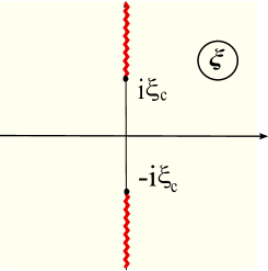
Figure 1: Analytic structure of $G_{\text{high}}(\xi)$ in the complex $\xi$-plane. The function has two singularities (YL edges) at $\xi=\pm i\xi_{c}$ and a third one at $\xi=\infty$ (the critical point). There are two cuts along the imaginary axis connecting the two YL edges and the critical point.

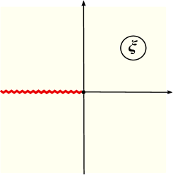
Figure 2: Analytic structure of $G_{\text{low}}(\xi)$. The function has two singularities, the critical point at $\xi=\infty$ and the low-temperature fixed point at $\xi\to 0$. The two singularities are connected by a branch cut extending from $-\infty$ to 0.

The numerical results obtained in [8] led the authors to a stronger assumption, which they referred to as ‘extended analyticity’, and which states that the Yang-Lee edge is the nearest singularity under the Langer branch cut. The extended analyticity suggests an interpretation of the YL edge as a quantum counterpart of the spinodal point in the classical theory of phase transitions. The classical low-temperature free energy is regular at $H=0$, but shows a branch-cut singularity at some negative $H=-H_{\rm SP}$, where the metastable phase becomes classically unstable. It was argued in [8] that the spinodal singularity does not disappear completely due to the quantum effects, but moves under the Langer cut and reappears as YL edge in the high-temperature phase. More recently, the numerical results of [8] were confirmed by a calculation based on the lattice formulation of the problem [11].

It is tempting to think that the qualitative picture of the analytic properties of the free energy, proposed in [8], applies to all statistical systems having a line of first order transitions ending at a second order transition point, and that the extended analyticity conjecture has a universal character. However, it is not clear how to address this issue directly. The Langer singularity is too weak to to be measured experimentally, and the TCFT approach used in [8] is sufficiently reliable only in the case of Majorana fermions.

On the other hand, it is known that some questions about the two-dimensional statistical systems can be answered by the following detour: formulate the system on a dynamical lattice, solve the problem exactly and then interpret the answer for the original system. This procedure is usually called ‘coupling to 2D quantum gravity’. Due to the enhanced symmetry, which erases the coordinate dependence of the correlation functions, the systems on dynamical lattices are much simple to resolve. This approach is based on the fact that there is a well established correspondence between the universal properties on the flat and dynamical lattices. On the dynamical lattice, the description of the critical points is given in terms of Liouville gravity [13]. The matter in Liouville gravity is given by the CFT describing the critical point of the statistical system on a flat lattice, while the Liouville field describes the fluctuations of the metric. The matter fields influence the geometry in a precise way, which is taken into account by accompanying Liouville vertex operators [14, 15, 16]. Knowing the correlation functions in 2D gravity, one can reconstruct the scaling dimensions of the matter operators. Moreover, the method based on coupling to 2D gravity is efficient also away from the critical points, where it makes possible to reconstruct the bulk and the boundary renormalization flow diagrams of the matter theory on a flat lattice, knowing the exact solution on dynamical lattice. The corresponding field theory is Liouville gravity perturbed by one or several fields.

The ising model is the only nontrivial example where the analytic properties of the free energy are known both on flat and dynamical lattices. The exact solution of Boulatov and Kazakov [17] shows that the Yang-Lee singularities appear also on a dynamical lattice and that near each YL singularity the critical behavior is that of a Yang-Lee CFT coupled to gravity [18, 19, 20]. However, it is not a priori clear if coupling to 2D gravity could be used to study the decay of the metastable vacuum by nucleation. Such a possibility was first explored in an unpublished work by Al. Zamolodchikov [21] and a subsequent work by A. and Al. Zamolodchikov [22].

The universal behavior of the Ising model on dynamical lattice is described by Ising Quantum Gravity (IQG), which represents a double perturbation of Liouville gravity with matter central charge $1/2$. The IQG is formally defined by the action

$${\cal A}_{\text{IQG}}={\cal A}_{c=1/2\ \text{Liouville gravity}}-t\,\int{\bf\varepsilon}(x)\,e^{2\alpha_{\varepsilon}\phi(x)}d^{2}x-h\,\int{\bf\sigma}(x)\,e^{2\alpha_{\sigma}\phi(x)}d^{2}x.$$ (1.4)

The exponents of Liouville dressing operators, $\alpha_{\varepsilon}=1/3$ and $\alpha_{\sigma}=5/6$, are such that the dressed matter operators become densities [15, 16]. The vacuum energy density of IQG must be of the form

$${\cal F}_{\text{IQG}}(t,h)=t^{3}{\cal G}(\xi),\qquad\xi=h/t^{5/2},$$ (1.5)

where the exponent $5/2=\alpha_{\sigma}/\alpha_{\varepsilon}$ is such that $\xi$ is invariant under rescalings of the metric. The vacuum energy density of the IQG, or the universal specific free energy of the discrete model, was extracted in [21] from the Bulatov-Kazakov exact solution [17]. For some normalization of the coupling constants, the universal free energy is given in parametric form by

$$\begin{aligned} {\cal F}_{\text{IQG}}(t,h)&=-{\textstyle{1\over 2}}\,u^{3}-\textstyle{3\over 4}\,u^{2}-\textstyle{3\over 4}\,h^{2}\,(u+t)^{-2}\,,\\ h^{2}\ \ &=u\,(u+t)^{4}.\end{aligned}$$ (1.6)

The scaling function ${\cal G}(\xi)$ defined in (1.5) is analytic on a Riemann surface representing a 5-sheet covering of the complex $\xi$-plane. The Riemann surface has a high-temperature (HT) sheet with two YL branch points at $\xi=\pm i\xi_{c}$ and two copies of the low-temperature (LT) sheet having a single cut starting at $\xi=0$ and going to infinity. The HT sheet is connected to the two LT sheets by two auxiliary sheets. In this way, the scaling functions ${\cal G}_{\text{high}}$ and ${\cal G}_{\text{low}}$ are identified with the restrictions of a single function ${\cal G}$ to the HT and the LT sheet of its Riemann surface.

In IQG, the discontinuity of ${\cal G}_{\text{low}}$ vanishes near the origin as $\xi^{3/2}$ and not exponentially, as predicted by the droplet model [21]. A field-theoretical explanation of the power law was given in [22], where Langer’s theory of the condensation point was adjusted to the case of a fluctuating metric. In the case of a flat lattice, the discontinuity across the Langer cut is related to the Boltzmann weight of the critical droplet of the true vacuum in the sea of the false vacuum (Fig.4). A. and Al. Zamolodchikov argued in [22] that in presence of gravity the droplets of the stable phase influence the metric, so that the perimeter of the boundary of a droplet grows slower than the square of the area (Fig. 4). This leads to a much faster decay of the unstable vacuum, which changes the character of the singularity at $\xi=0$. This phenomenon was named by the authors of [22] ‘critical swelling’.

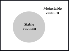
Figure 3: A critical droplet of the true vacuum in the sea of false vacuum.

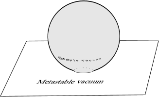
Figure 4: The metric of the critical droplet in presence of gravity.

The work [22] gave a convincing evidence that the Langer singularity in IFT has its counterpart in IQG, and that both singularities are due to the presence of a weakly metastable state. Is it possible to extend the IFT/IQG correspondence to more general spin systems? In fact, the analysis of [22] applies to any droplet model in presence of gravity. Due to the critical swelling, the Boltzmann weight of the critical droplet is expected to behaves as a power, $h^{g_{\text{low}}}$, where the exponent $g_{\text{low}}$ is determined by the conformal anomaly in the low-temperature phase $c_{\text{low}}$. The saddle point analysis of [22] gives $g_{\text{low}}=-{1\over 6}c_{\text{low}}$ in the classical limit $c_{\text{low}}\to-\infty$, where the fluctuations of the Liouville field can be neglected. The authors of [22] conjectured (we will refer to this as Z-Z conjecture) that the exact nucleation exponent $g_{\text{low}}$ is related to the central charge of the stable phase as follows,

$$g_{\text{low}}={p\over p-1}\quad\text{for}\quad c_{{\text{low}}}=1-{6\over p(p-1)}.$$ (1.7)

In the case of IQG, $c_{{\text{low}}}=0$ and $g_{\text{low}}=3/2$, which is in agreement with the singularity of ${\cal G}_{\text{low}}$ at $\xi=0$. If the conjecture (1.7) is confirmed, this would open the possibility to study the analytical properties of the free energy of a spin systems on a flat lattice, in particular in what concerns the Langer and YL singularities, using its exact solution on a dynamical lattice.

The conjecture (1.7) about the nucleation rate exponent can be tested by looking for more solvable examples among the dynamical lattice statistical systems, which exhibit metastability and have non-trivial massless modes in the stable vacuum. In this paper we argue that the $O(n)$ loop model in external magnetic field is such a system.

Technically the main result of this paper is the explicit expression for the specific free energy of the gravitational $O(n)$ model in the continuum limit, which we obtain using the correspondence with a large $N$ matrix model [23]. The main body of the text is devoted to the interpretation of this exact solution. In Sect. (2) we formulate the expected analytic properties of the free energy of the $O(n)$ loop model on a flat lattice as well as the the non-perturbative effects associated with the existence of a hypothetical metastable vacuum. In Sect. (3) we perform the same analysis of the gravitational $O(n)$ model. In particular, assuming the existence of a metastable state and the conjectured nucleation exponent (1.7), we reproduce the form of the series expansion of the free energy of the low-temperature phase at $h=0$. In Sect. 4 we verify that the exact expression for the free energy possesses the expected analytic properties, which justifies the assumption of the existence of a weakly metastable state in the $O(n)$ loop model. Our result verify the Z-Z conjecture for the whole spectrum $-\infty<c<1$ of the central charge of the matter field. Since the paper is somewhat technical, below we give a short summary of our results.

$\diamond\diamond\diamond$

The $O(n)$ loop model [24, 25] has a geometrical formulation in terms of nonintersecting loops with fugacity $n$. In presence of magnetic field $H$, the geometrical expansion involves also open lines with fugacity $H^{2}$, as in the example shown in Fig. 6. The temperature $T$ controls the total length of the linear polymers. In the conformal window $-2<n<2$, the theory has a conformal invariant critical point at $T=T_{c}$ and $H=0$, described by a CFT with central charge [26],

$$c_{{}_{\rm crit}}=1-{6\over p(p+1)},$$ (1.8)

where $p$ is related to the dimensionality $n$ by

$$n=2\cos{\pi\over p},\qquad p\geq 1.$$ (1.9)

The critical $O(n)$ model covers the whole one-parameter family of universality classes having massless modes in the low-temperature phase, with a central charge $-\infty<c\leq 1$.

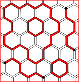
Figure 5: A polymer configuration on a honeycomb lattice

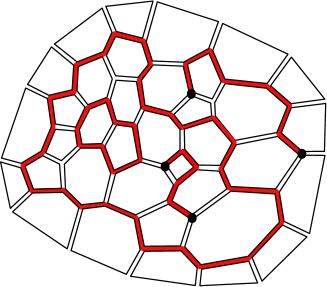
Figure 6: A polymer configuration on a planar graph with the topology of a disk

The phase diagram of the $O(n)$ loop model is similar to that of the Ising model, which corresponds to the particular case $n=1$, or $p=3$. For $T>T_{c}$ the typical linear polymer is short and the theory has a mass gap. Nienhuis [25] showed, using the mapping to other solvable lattice models and the Coulomb gas techniques, that for $T<T_{c}$ and $H=0$ the model is characterized by a massless low-temperature (LT) phase, also known as a phase of dense loops. The LT phase of the $O(n)$ vector model is described by another CFT with central charge

$$c_{\text{low}}=1-{6\over p(p-1)}.$$ (1.10)

The vicinity of the critical point ($T=T_{c},H=0$) is described by the ‘$O(n)$ field theory’, or shortly $O_{n}$FT, which is a perturbation of the CFT with central charge (1.8). The $O(n)$ field theory is formally defined by the action

$${\cal A}_{{{O_{n}\text{FT}}}}={\cal A}_{{{}_{\rm crit}}}-h\int{\rm s}(x)\,d^{2}x-t\int\varepsilon(x)\,d^{2}x\,,$$ (1.11)

where ${{\rm s}}$ and $\varepsilon$ are the conformal fields generating the perturbations respectively in the magnetic field $h\sim H$ and in the temperature $t\sim T-T_{c}$. When $p$ is an odd integer, $p=2m-1$, this action describes the unitary minimal conformal theory ${\cal M}_{2m-1,2m}$ perturbed by the two primary fields

$$\hskip 56.9055pt\varepsilon=\Phi_{1,3}\,,\quad{\rm s}=\Phi_{m,m}\hskip 56.9055pt(m={\textstyle{1\over 2}}(p+1))\,.$$ (1.12)

The Ising field theory corresponds to $m=2$, or $n=1$. The thermal flow generated by $\varepsilon$ ends, depending on the sign of the temperature coupling, at a massive theory in the HT regime, or at a CFT with the lower central charge (1.10) in the LT regime [29]. For a general $p>1$, the $O(n)$ field theory does not exist as a local field theory, but it has nonetheless an unambiguous definition in terms of grand canonical ensemble of linear polymers on the lattice.

In Sect. 2 we speculate about the analytic properties of the specific free energy of ${O_{n}\text{FT}}$, assuming that there exists a weakly metastable state and Langer singularity at least in some finite vicinity of the point $p=3$. Since the free energy depends analytically on the parameter $p$, this is a natural assumption, although for $p\neq 3$ we do not see any geometrically transparent picture of the nucleation mechanism. We give a heuristic argument about the form of the Langer singularity for $p\neq 3$. The non-perturbative corrections should be of the form

$$F_{\text{nonpert}}\sim f\ \exp(-\text{const}/f),\qquad f\sim|h|^{1/(1-\Delta_{\rm s}^{\text{low}})},$$ (1.13)

where $\Delta_{\rm s}^{\text{low}}$ is the conformal dimension of the $O(n)$ spin field ${\rm s}$ in the low-temperature phase.

As in the case of IFT, the specific free energy is determined by two different scaling functions in the HT and in the LT regimes:

$$F(t,h)=\begin{cases}\ \ t^{p+1\over 2}\ G_{\text{high}}(\xi),\qquad\xi=t^{-\omega_{0}}h\quad&\text{if }\quad t>0,\\ &\\ (-t)^{p+1\over 2}\ G_{\text{low}}(\zeta),\quad\zeta=(-t)^{-\omega_{0}}h\quad&\text{if}\quad t<0,\end{cases}$$ (1.14)

where the power ${p+1\over 2}$ and the exponent

$$\omega_{0}\equiv{1-\Delta_{{\rm s}}\over 1-\Delta_{\varepsilon}}={(3p+1)(5p+3)\over 32p}\,$$ (1.15)

are determined by the conformal weights $\Delta_{\varepsilon}=\bar{\Delta}_{\varepsilon}$ and $\Delta_{\rm s}=\bar{\Delta}_{\rm s}$ respectively of $\varepsilon$ and ${\rm s}$ at the critical point. The function $G_{\text{high}}$ has a couple of Yang-Lee branch points on the imaginary axis and is analytic at the origin, while the function $G_{\text{low}}$ is expected to have an essential singularity at $\zeta=0$. We argue that the domain of analyticity of $G_{\text{low}}(\zeta)$ is the wedge $|\arg(\zeta)|<\pi(1-\Delta_{\rm s}^{\text{low}})$. The scaling functions $G_{\text{high}}$ and $G_{\text{low}}$ are analytically related at infinity and can be expressed through a third scaling function $\Phi(\eta)$, where $\eta=h^{-1/\omega_{0}}\,t$ is the dimensionless temperature coupling.

In Sect. 3 we formulate the the analytic properties of the free energy of $O(n)$ quantum gravity, or shortly ${O_{n}\text{QG}}$, which describes the continuum limit of the $O(n)$ model on a dynamical lattice. The geometrical expansion in this case involves non-intersecting loops and lines on planar graphs as the example in Fig. 6. ${O_{n}\text{QG}}$ is formally defined as a perturbation of Liouville gravity with matter central charge (1.8) by the action

$$\delta{\cal A}_{{O_{n}\text{QG}}}=-t\,\int\varepsilon(x)\,e^{2\alpha_{\varepsilon}\phi(x)}d^{2}x-h\,\int{\rm s}(x)\,e^{2\alpha_{\rm s}\phi(x)}d^{2}x,$$ (1.16)

which generalizes (1.4). The vacuum energy of ${O_{n}\text{QG}}$ must be of the form

$${\cal F}(t,h)=\begin{cases}\ \ t^{p}\ {\cal G}_{\text{high}}(\xi),\qquad\xi=t^{-\omega}h\quad&\text{if }\quad t>0,\\ &\\ (-t)^{p}\ {\cal G}_{\text{low}}(\zeta),\quad\zeta=(-t)^{-\omega}h\quad&\text{if}\quad t<0,\end{cases}$$ (1.17)

where $\omega$ is the ratio of the Liouville dressing exponents associated with the two perturbing operators,

$$\omega={\alpha_{\rm s}\over\alpha_{\epsilon}}={3p+1\over 4}.$$ (1.18)

Again, the functions ${\cal G}_{\text{high}}$ and ${\cal G}_{\text{low}}$ are related analytically at infinity and can be expressed in terms of a third scaling function $\Phi(\eta)$, where $\eta=h^{-1/\omega}t$ is the dimensionless temperature. This determines the form of the expansion at infinity

$${\cal G}_{\text{high}}(\xi)=\sum_{j=0}^{\infty}\Phi_{j}\ \xi^{1-j\alpha_{\epsilon}\over\alpha_{\rm s}},\qquad{\cal G}_{\text{low}}(\zeta)=\sum_{j=0}^{\infty}(-1)^{j}\ \Phi_{j}\ \zeta^{1-j\alpha_{\epsilon}\over\alpha_{\rm s}}.$$ (1.19)

At the origin the function ${\cal G}_{\text{high}}$ is analytic, while ${\cal G}_{\text{low}}$ is expected, according to [22], to have a power-like singularity. The leading term in the expansion is $f\sim\zeta^{1/\alpha_{\rm s}^{\text{low}}}$, where $\alpha_{\rm s}^{\text{low}}$ is the Liouville exponent associated with the magnetic operator in the low-temperature phase. The Z-Z conjecture concerns the subleading term, which should be $\sim f^{\,g_{\text{low}}}$, with $g_{\text{low}}$ given by (1.7). We develop further the arguments of [22] by considering the contributions of droplets-within-droplets configurations. In this way we were able to predict not only the first two terms, but the form of the whole series expansion the scaling function ${\cal G}_{\text{low}}$,

$$\begin{aligned} {\cal G}_{\text{low}}(\zeta)&=\tilde{\cal G}_{0}+C_{1}\,f+C_{2}\,{f}^{\,g_{\text{low}}}\,\big{(}1+C_{3}\,{f^{\,g_{{\text{low}}}}\over\zeta}+\dots\big{)}\\ &=\tilde{\cal G}_{0}+\sum_{n\geq 0}\tilde{\cal G}_{n}\ \zeta^{{4(p-1)\over 3p-1}+{4n\over 3p-1}}.\end{aligned}$$ (1.20)

In Sect. 4 we compare the speculations of sections 2 and 3 about the behavior of the $O(n)$ free energy with the exact solution, obtained for the microscopic realization of ${O_{n}\text{QG}}$ as the $O(n)$ loop model on a dynamical lattice. The derivation, based on the correspondence with the $O(n)$ matrix model, is given in Appendix A. The specific free energy ${\cal F}(t,h)$ was found in a parametric form,

$$\begin{aligned} {\cal F}(t,h)=&-{y^{p}\over 2}+t\,{y^{p-1}\over 2(1-{1\over p})}-h^{2}\,{y^{-(p+1)/2}\over 1+{1\over p}}\,,\\ h^{2}\ =&\ y^{(3p-1)/2}(y-\,t).\end{aligned}$$ (1.21)

For $p=3$ the equation for the $O(n)$ free energy coincides, up to a shift by a term $\sim t^{3}$, with Boulatov-Kazakov solution of IQG, eq. (1.6).

From the solution (1.21) we find the scaling functions ${\cal G}_{\text{high}}$ and ${\cal G}_{\text{low}}$. They represent two different branches of the same meromorphic function ${\cal G}$, which is defined as the analytic continuation of ${\cal G}_{\text{high}}(\xi)$ under the YL cuts. The function ${\cal G}(\xi)$ has the symmetries

$${\cal G}(\xi)={\cal G}(-\xi)=\overline{{\cal G}(\bar{\xi})},$$ (1.22)

which are inherited by those of the function ${\cal G}_{\text{high}}$ and which preserve by construction the HT sheet. Starting from the HT sheet and taking different paths, one can achieve (for general $p$) four different copies of the LT sheet, related by the symmetries (1.22). The HT and the LT sheets are connected by a finite number of auxiliary sheets. The extended analyticity assumption, which is fulfilled here, means that there is no additional singularities on the connecting sheets.

We computed the series expansions of ${\cal G}_{\text{low}}$ and ${\cal G}_{\text{high}}$ at $\zeta=0$ and at $\zeta=\infty$. The expansion of ${\cal G}_{\text{low}}$ at the origin is indeed of the form (1.20), which confirms the Z-Z conjecture in its stronger form used in Sect. 3 as well as the existence of Langer singularity at the origin associated with the presence of a metastable state. If the gravitational field is ‘switched off’, the power-like singularity at $\zeta=0$ should turn into an essential singularity associated with this metastable state. Let us stress that we expect Langer-type singularity only in the $O(n)$ loop model which has a representation in terms of a gas of non-intersecting polymers. The conventional $O(n)$ model should not have such a singularity.

To summarize, in this work we argue that Langer’s singularity in presence of small magnetic field, originally observed in the Ising model, is in fact a general feature of the $O(n)$ loop models. We are quite confident in our conclusions when $0<n<2$, while in the interval $-2<n<0$, where the loop gas does not have statistical interpretation, the situation is less clear. Our exact expression for the free energy of the gravitational $O(n)$ model presents a strong evidence about the existence of a metastable state in the low-temperature phase and confirms the Z-Z conjecture about the decay rate of the metastable vacuum in presence of gravity [22] in the case when the stable phase has non-zero central charge. We found that the scaling function ${\cal G}(\xi)$ for the free energy of the $O(n)$ loop model on a dynamical lattice has a pair of Yang-Lee singularities on the high-temperature sheet, a Langer-type singularity of the expected form on the low-temperature sheet, and no additional singularities on the connecting sheets. In this sense the scaling function obeys the ‘extended analyticity’ assumption of Fonseca and Zamolodchikov [8]. However, it is not clear if this property will remain true for the theory on a flat lattice. This is a very important question which deserves further study.

2 The vacuum energy of the $O(n)$ field theory

The analytic properties of the free energy of of $O_{n}FT$, except Langer singularity, follow immediately from the known scaling behavior near the critical points, where the theory becomes conformal invariant, and the assumption that on the first sheet there are no other singularities than the critical points. These predictions are in accordance with the numerical results for the cases $n=1$ [8, 11] and $n=0$ [30]. In contrast, as we already discussed, we do not have direct arguments in favor of the presence of Langer singularity. This is a conjecture which is justified by the exact solution of the model coupled to gravity.

2.1 Continuous transitions and effective field theory on a regular lattice

The local fluctuating variable in the $O(n)$ loop model [24, 25, 31] is an $n$-component vector $\vec{S}(r)$ with unit norm, associated with the vertices $r$ of the honeycomb lattice, and interacting in an isotropic way along the links $<\!\!r,r^{\prime}\!\!\!>$. In the presence of a constant magnetic field $\vec{H}$, the energy of a spin configuration is defined by the “geometric” hamiltonian

$${\cal H}[\{\vec{S}\}]=-\sum_{<r,r^{\prime}>}\log\left(T+\vec{S}(r)\cdot\vec{S}(r^{\prime})\right)-\sum_{r}\log\left(1+\vec{S}(r)\cdot\vec{H}\right).$$ (2.1)

The logarithmic form of the nearest neighbor interaction leads to a simple graphical expansion which generalizes that of the Ising model and can be mapped to a solvable vertex model. The partition function is defined as the trace (the integral over all spin configurations)

$${\cal Z}_{{}_{O(n)}}(T;\Gamma)={\rm Tr}\ e^{-{\cal H}[\{\vec{S}\}]},$$ (2.2)

where by the $O(n)$ symmetry ${\rm Tr}(S_{a}S_{b})=\delta_{a,b}$ and ${\rm Tr}(S_{a})={\rm Tr}(S_{a}S_{b}S_{c})=0$. Expanding the integrand as a sum of monomials and using the rules above one can write the high temperature expansion of the partition function as the grand canonical ensemble of non-intersecting polymers of variable length. There are two kinds of polymers: loops with activity $n$ and open lines with activity $H^{2}$, where $H=|\vec{H}|$. Apart of the activity, the Boltzmann weight of each polymer is equal to $T^{-L}$, where $L$ is the length, defined as the number of links covered by the polymer. The high temperature expansion of the partition function is a triple series in $n$, $1/T$ and $H^{2}$,

$${\cal Z}_{{}_{O(n)}}(T,\vec{H})=\sum_{\text{polymers }}\;(1/T)^{L_{\rm tot}}\,n^{\#\text{loops}}\,H^{2\#\,\text{open lines}}.$$ (2.3)

The temperature coupling $T$ controls the total length $L_{\rm tot}$ of the polymers (the number of links covered by loops or open lines). An example of a polymer configuration is given in Fig. 6. The geometrical expansion (2.3) of the $O(n)$ model allows to consider the number of flavors $n$ as a continuous parameter.

When $\vec{H}=0$, the $O(n)$ loop model is known to have a continuous transition in the window $-2\leq n\leq 2$, where $n$ can be parametrized by eq. (1.9). The phase diagram of the loop gas on the honeycomb lattice was first established by Nienhuis [25]. At the critical temperature $T_{\text{crit}}=2\cos\frac{\pi(p-1)}{4p}$ the loop gas model is solvable and described by a CFT with central charge (1.8). This point is usually referred as the ‘dilute’ phase. For $T>T_{\text{crit}}$, the theory has a mass gap. The low-temperature, or ‘dense’, phase $T<T_{\text{crit}}$ represents a massless flow toward an attractive fixed point at $T_{\text{low}}=2\sin\frac{\pi(p-1)}{4p}$. At this point the theory is again solvable and described by a CFT with smaller central charge $c_{\text{low}}$ defined by (1.10).

The spectrum of the degenerate primary fields in the critical and in the low-temperature CFTs is given respectively by

$$\Delta_{r,s}={(r(p+1)-sp)^{2}-1\over 4p(p+1)},\qquad\Delta_{r,s}^{\text{low}}={(rp-s(p-1))^{2}-1\over 4p(p-1)}\,,$$ (2.4)

where $r$ and $s$ are integers. The thermal operator $\varepsilon$, which counts the total length of the polymers in the expansion (2.3), can be identified with the degenerate field $\Phi_{1,3}$. Added to the action, it generates a mass of the loops. The spin operator ${\rm s}$ coupled to the magnetic field corresponds to a degenerate primary field only if $p$ is an odd integer,

$$p=2m-1.$$ (2.5)

However, it is convenient to extend the Kac parametrization (2.4) also for non-integer $r$ and $s$. Then the magnetic field can be identified with the field of conformal dimensions $\Delta_{\rm s}=\bar{\Delta}_{\rm s}=\Delta_{m,m}$, with $m={1\over 2}(p+1)$. The magnetic operator is the first of an infinite series of $L$-leg operators $\Phi_{Lm,Lm}\ (L=1,2,\dots)$ [32]. Explicitly, the conformal weights of the thermal and spin operators are given by

$$\Delta_{\varepsilon}=\Delta_{1,3}={p-1\over p+1},\quad\Delta_{\rm s}=\Delta_{{p+1\over 2},{p+1\over 2}}={1\over 16}\ {(p+3)(p-1)\over p(p+1)}.$$ (2.6)

Both operators are relevant. The $O(n)$ field theory, which describes the continuum limit of the Hamiltonian (2.1), is formally defined by the action (1.11), where

$$t\sim T-T_{\text{crit}},\quad h\sim|\vec{H}|.$$ (2.7)

parametrize the vicinity of the critical point of the lattice model. When $n=1$, or $p=3$, this action coincides with the action (1.1) for the Ising field theory. Depending on the sign of the temperature, the perturbation by the thermal operator $\varepsilon$ generates a flow toward the massive or to the dense phase.

As we already mentioned in Sect. 1, the low-temperature phase of the $O(n)$ loop model defined by the Hamiltonian (2.1) does not contain Goldstone modes. This is in contrast with the standard $O(n)$ model [33, 34], which is defined by the Hamiltonian

$${\cal H}[\{\vec{S}\}]=-{1\over T}\sum_{<r,r^{\prime}>}\vec{S}(r)\cdot\vec{S}(r^{\prime})-\sum_{r}\vec{S}(r)\cdot\vec{H}.$$ (2.8)

In the case of the Ising model ($n=1$), the Hamiltonians (2.1) and (2.8) are equivalent, up to a redefinition of the two couplings. For general $n\in[-2,2]$, the two Hamiltonians are supposed to share the same universal properties in the high temperature phase and at the transition point, while the low temperature phases of the two models are believed to be different [28]. For $T<T_{c}$, the $O(n)$ symmetry of the model with Hamiltonian (2.8) is spontaneously broken to $O(n-1)$, which leads to a massless Goldstone phase with central charge $\tilde{c}_{\text{low}}=n-1$. (Since the model is non-unitary, the Mermin-Wagner theorem does not apply here.) In contrast, the low-temperature phase of the model with Hamiltonian (2.1) exhibits unbroken $O(n)$ symmetry.

In terms of the geometrical expansion, the Goldstone phase appears when the loops are allowed to intersect. The Hamiltonian (2.1) of the $O(n)$ loop model is designed in such a way that the intersections are strictly forbidden. This is why the Goldstone modes do not appear. It is argued in [28] that an arbitrarily small perturbation that allows intersections would cause a crossover to the generic Goldstone phase.

2.2 High-temperature regime

In the high-temperature phase of the $O(n)$ model, the deformation (1.11) with $t>0,h=0$ describes, from short to long distance scales, the flow to a massive theory. For finite $t$, the specific free energy, or the vacuum energy density of the $O(n)$ field theory, scales as

$$F(t,0)\sim t^{1-\Delta_{\varepsilon}}=t^{p+1\over 2}\qquad(h=0,\ t>0).$$ (2.9)

For finite $h$ and $t$, the specific free energy must have the scaling form

$$F(t,h)=t^{p+1\over 2}G_{\text{high}}(\xi),$$ (2.10)

where the scaling function $G_{\text{high}}$ depends on the dimensionless variable

$$\xi=t^{-\omega_{0}}h,\quad\omega_{0}={1-\Delta_{h}\over 1-\Delta_{t}}={(3p+1)(5p+3)\over 32p}\,.$$ (2.11)

When $p$ is an odd integer, as in the case of the IFT, one should take the derivative of (2.10) in $p$,

$$F(t,h)\sim t^{m}\log t+t^{m}\hat{G}_{{\text{high}}}(\xi),\qquad p=2m-1=\text{odd integer}.$$ (2.12)

Since for a finite positive $t$ the theory has a mass gap, the scaling function should be analytic at $\xi=0$. The high temperature expansion (2.3) involves only even powers of the magnetic field, which means that $G_{\text{high}}$ is an even function of $\xi$ in the vicinity of $\xi=0$,

$$G_{\text{high}}(\xi)=G_{0}+G_{2}\xi^{2}+G_{4}\xi^{4}+\dots\quad\text{for}\ \ \xi\to 0.$$ (2.13)

On the other hand, the large $h$ finite and $t=0$ the theory is again massive with correlation length determined by the conformal weight $\Delta_{\rm s}$. Hence the asymptotic behavior of the scaling function at infinity is

$$G_{\text{high}}(\xi)\sim\xi^{1/(1-\Delta_{\rm s})}+\cdots\quad\text{ for}\ \ \xi\to\infty.$$ (2.14)

The function $G_{\text{high}}(\xi)$ can be analytically continued for complex values of $\xi$. Obviously the scaling function has branch points at some finite $\xi$, otherwise the two asymptotics (2.13) and (2.14) would be incompatible. As argued in [34], the general $O(n)$ model exhibits in the HR regime the same analytical properties than the Ising model: the zeros of the partition are situated along the imaginary axis, and an infinite strip centered around the real axis is free of zeros. Then, the free energy would have two symmetric branch cuts on the imaginary axis, extending from $\pm i\xi_{c}$ to $\pm i\infty$, as is shown in Fig. 2. The branch points correspond to the two Yang-Lee edges, and in the vicinity of $\xi=\pm i\xi_{c}$ the $O(n)$ field theory is expected to be described by the minimal CFT $\mathcal{M}_{2,5}$ with a central charge $c^{{}_{{}^{\text{YL}}}}=-22/5$ [4]. The Yang-Lee CFT has only one relevant operator $\Phi_{1,2}$ with the conformal dimension $\Delta^{{}_{{}^{\text{YL}}}}_{1,2}=-1/5$. The dimension of the corresponding coupling constant is $1-\Delta_{1,2}^{{}_{{}^{\text{YL}}}}=6/5$ and one expects, as in [8], that near the YL branch points $G_{\text{high}}(\xi)$ behaves as

$$G_{\text{high}}(\xi)=g_{A}(\xi)+g_{B}(\xi)\,\left(\xi_{c}^{2}+\xi^{2}\right)^{5/6}+\dots,$$ (2.15)

with $g_{A}$ and $g_{B}$ being regular functions of $\xi$.

2.3 Low-temperature regime

In the LT regime ($t<0$) the theory flows toward a CFT with the central charge $c_{\text{low}}$ given in (1.10) [29, 35]. The perturbation of the low-temperature CFT at $t\to-\infty,h=0$ is driven by the operators $\varepsilon$ and ${\rm s}$ with conformal weights

$$\Delta^{\text{low}}_{\varepsilon}=\Delta_{3,1}^{\text{low}}={p+1\over p-1},\quad\Delta^{\text{low}}_{\rm s}=\Delta_{{p-1\over 2},{p-1\over 2}}^{\text{low}}={1\over 16}\ {(p-3)(p+1)\over p(p-1)}$$ (2.16)

and coupled respectively to $-1/t$ and $h$. The energy becomes an irrelevant operator, while the magnetic field remains relevant. A finite perturbation at $t\to-\infty$ with this operator leads to a massive theory with specific free energy

$$F(t,h)\sim h^{1/(1-\Delta^{\text{low}}_{\rm s})}\qquad(t\to-\infty).$$ (2.17)

For the Ising model $(p=3)$ the low-temperature phase contains no degrees of freedom, $c_{\text{low}}=0$ and $\Delta_{\rm s}^{\text{low}}=0$. The free energy is $F\sim h$ and the magnetization

$$\bar{\rm s}=-\partial F/\partial h$$ (2.18)

is a constant. The dimension of the magnetic operator becomes negative for $p<3$. Accordingly, the magnetization $\bar{\rm s}$ vanishes at $h\to 0$ for $p>3$ and diverges as $h^{\Delta_{\rm s}^{\text{low}}/(1-\Delta_{\rm s}^{\text{low}})}$ for $p<3$. In particular, for $p=2$, which corresponds to the case of the dense polymers, the specific free energy diverges as $F\sim h^{32/35}$. This scaling behavior has been tested and confirmed numerically by Saleur [30]. In the opposite limit, $h\to\infty$, the free energy is again given by (2.14). On the other hand, for finite negative $t$ and $h=0$ the free energy behaves as

$$F(t,h)\sim(-1/t)^{1/(1-\Delta^{\text{low}}_{\varepsilon})}=(-t)^{p+1\over 2}\qquad(h=0,\,t<0).$$ (2.19)

For finite values of $h$ and $t$ the vacuum energy is of the form

$$F(t,h)=(-t)^{p+1\over 2}\,G_{{\text{low}}}(\zeta),$$ (2.20)

where $G_{\text{low}}$ is the scaling function in the low-temperature phase and $\zeta$ is defined as

$$\zeta=(-t)^{-\omega_{0}}h\,.$$ (2.21)

At small $\zeta$ the scaling function $G_{\text{low}}$ has asymptotic behavior

$$G_{\text{low}}(\zeta)\sim\tilde{G}_{0}+\tilde{G}_{1}\,\zeta^{1/(1-\Delta_{\rm s}^{\text{low}})}+\dots\quad\text{for}\ \zeta\to 0,$$ (2.22)

while at infinity $G_{\text{low}}\sim\zeta^{1/(1-\Delta_{\rm s})}$. By construction the function $G_{\text{low}}(\zeta)$ is real for $\zeta>0$. The constant term in (2.22) is in general different than the one in (2.13). Since the susceptibility and the magnetization are positive, we have $\tilde{G}_{0}>0$ and $\tilde{G}_{1}<0$. The relation between $G_{\text{low}}$ and $G_{\text{high}}$ will be obtained in Sect. 2.5.

2.4 Langer singularity

In the Ising model ($p=3$) the scaling function $G_{\text{low}}$ is expanded in the integer powers of $\zeta$, but the power series is asymptotic. The analytical continuation of the free energy from positive $\zeta$ has an exponentially small purely imaginary discontinuity on the negative axis, which is explained by the presence of a metastable state for small negative $\zeta$. In the language of QFT, one could say that the theory contains a global resonance state with complex energy, the ‘false vacuum’. The imaginary part of the specific free energy can then be interpreted as the decay rate per unit time and volume of this resonance state [36][9][10]. Langer [5, 6] developed a systematic approach, based on the earlier droplet models, to evaluate the discontinuity $\delta F=2i\Im F$ of the free energy on the negative axis. The latter decays exponentially for small magnetic field, $\delta F\sim\exp({-{\rm const}/|\zeta|})$.

By construction, the free energy and the correlations in the $O(n)$ loop model are analytic in $p$. If the perturbative expansion of the free energy at $p=3$ is asymptotic, it will be asymptotic also in the vicinity of $p=3$. Therefore it is very likely that a metastable state and Langer type singularity should exist also for $p\neq 3$. This conjecture will be later confirmed by the exact solution on dynamical lattice. Unfortunately it is not clear how to characterize geometrically the true and the false vacuum within the loop gas representation, even in the Ising case $p=3$.

In the Ising model the energy gap between the stable and the metastable vacuum is evaluated by analytically continuing the free energy to negative values of $h$. For general $p$ the leading behavior of the free energy for small $h$ is no more linear in $\zeta$,

$$F(t,h)=(-t)^{p+1\over 2}\left(\tilde{G}_{0}+\tilde{G}_{1}\zeta^{2\nu}+\dots\right),\quad 2\nu\stackrel{{\scriptstyle\text{def}}}{{=}}1/(1-\Delta_{\rm s}^{\text{low}}),$$ (2.23)

and the metastable state should be reached by analytical continuation to the rays $\arg(\zeta)=\pm\pi/2\nu$ in the complex $h$-plane. Here the free energy is again real and the gap

$$\begin{aligned} f(t,\zeta)\equiv F(t,e^{\pm i\pi/2\nu}h)-F(t,h)\end{aligned}$$ (2.24)

is positive. Langer’s theory [5] predicts a nnon-perturbative, exponentially small in $f$, imaginary part of $F$, equal to the decay rate $\Gamma$ (per unit volume and unit time) of the metastable vacuum,

$$F(t,e^{i\pi/2\nu}h)-F(t,e^{-i\pi/2\nu}h)\sim i\Gamma.$$ (2.25)

To evaluate the leading exponential factor, assume that initially the two-dimensional plane is filled with the metastable vacuum with specific free energy $F+f$ and imagine a hypothetical stochastic process which allows the statistical system to develop in time. The decay of the metastable vacuum will then occur through spontaneous formation of droplets of the stable phase in the “sea” of metastable phase. The Boltzmann weight of a droplet of area $A$ and perimeter $L$ is

$$W_{A,L}\sim e^{Af-L\sigma},$$ (2.26)

where ${\rm s}$ is the surface tension at the boundary of the droplet. The surface tension scales as $\sigma=\sigma_{0}(-t)^{p+1\over 4}$, where ${\rm s}_{0}$ is a numerical coefficient. Assuming that the drops are approximatively round, $A=L^{2}/4\pi$, the integral in $L$ is saturated by the saddle point $L_{s.p.}=2\pi\sigma/f$. The saddle point value gives the size of the ‘critical droplet’, which can trigger a decay of the metastable state. For droplets larger than the critical droplet the bulk energy starts to decrease faster than the surface energy grows and the droplet energetically favorable to grow. The leading factor in the decay rate $\Gamma$ is the Boltzmann weight of the critical droplet. A more refined calculation [37], taking into account the fluctuations of the form of the droplets, gives also the pre-exponential factor,

$$\begin{aligned} \Gamma\sim{f}\ e^{-\pi\sigma^{2}/f}.\end{aligned}$$ (2.27)

Therefore, with the assumptions we made, the scaling function $G_{\text{low}}(\zeta)$ for the LT regime develops an essential singularity $\sim|z|^{2\nu}e^{-|\zeta|^{2\nu}}$ at the origin. The function $G_{\text{low}}(\zeta)$ is analytic in the $\zeta$-plane with a cut starting at $\zeta=0$, which can be placed along one of the rays $\arg(\zeta)=\pm\pi/2\nu$, where the discontinuity of the leading perturbative term vanishes, or along the negative axis, which will be our choice in the following.

2.5 The scaling function $\Phi(\eta)$

The functions $G_{\text{high}}(\xi)$ and $G_{\text{low}}(\zeta)$, although defined for two different phases, must be analytically connected in the regime where the magnetic field is sufficiently large compared to the temperature. In this regime it is useful to introduce the dimensionless temperature

$$\eta=h^{-1/\omega_{0}}\,t,$$ (2.28)

with $\omega_{0}$ was defined in (1.15), and a new scaling function $\Phi(\eta)$ by

$$F(t,h)=h^{1/(1-\Delta_{\rm s})}\,\Phi(\eta).$$ (2.29)

This new variable is suited to study the analytical property of the free energy in terms of the temperature. In particular, it allows the description of the neighborhood of the critical point where $t\sim 0$. In the regime $t>0$ and $h>0$, the variable $\eta$ is related to $\xi$ by

$$\eta=\xi^{-1/\omega_{0}}$$ (2.30)

and the new scaling function is expressed in terms of $G_{\text{high}}(\xi)$ as

$$\Phi(\eta)=\eta^{{1\over 1-\Delta_{\varepsilon}}}\,G_{\text{high}}(1/\eta^{\omega_{0}}),\qquad(\eta>0).$$ (2.31)

Similarly, in the regime $t<0$ and $h>0$

$$\eta=-\,\zeta^{-1/\omega_{0}}$$ (2.32)

and

$$\Phi(\eta)=(-\eta)^{{1\over 1-\Delta_{\varepsilon}}}\,G_{\text{low}}(1/(-\eta)^{\omega_{0}}),\qquad(\eta<0).$$ (2.33)

(When $p$ is an odd integer, the above relations are slightly modified. They are obtained by taking the derivative in $p$ and using the definition (2.12).)

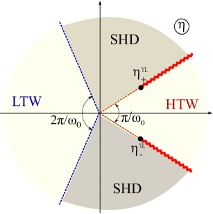
Figure 7: Principal sheet of the $\eta$-plane for the scaling function $\Phi(\eta)$. The LT wedge $|\arg(-\eta)|<{2\pi/\omega_{0}}$ is the image of the principal sheet of the scaling function $G_{\text{low}}(\zeta)$. The HT wedge $|\arg(\eta)|<{\pi/2\omega_{0}}$ is the image of the right half plane of the principal sheet of $G_{\text{high}}(\xi)$. The two sectors SHD separating the LT and the HT wedges are the ‘shadow domain’ where the analytic properties of $\Phi(\eta)$ are not known. In [8] it was conjectured (for $p=3$) that the function $\Phi(\eta)$ is analytic also in the shadow domain.

Since for $h\neq 0$ the theory has a mass gap, the free energy $F(t,h)$ should be analytic in the temperature $t$ in some finite strip around the real axis. Therefore the scaling function $\Phi(\eta)$ is represented by a power series

$$\Phi(\eta)=\Phi_{0}+\Phi_{1}\,\eta+\Phi_{2}\eta^{2}+\dots$$ (2.34)

with a finite radius of convergence near $\eta\sim 0$. According to (2.31) and (2.33), the coefficients $\Phi_{k}$ of the series (2.34) determine the large expansion of the scaling functions $G_{\text{high}}(\xi)$ and $G_{\text{low}}(\zeta)$ at infinity,

$$\begin{aligned} G_{\text{high}}(\xi)&=&\xi^{{1\over 1-\Delta_{\rm s}}}\Phi(\xi^{-1/\omega_{0}})\quad=\sum_{j=0}^{\infty}\Phi_{j}\ \xi^{1-j(1-\Delta_{\varepsilon})\over 1-\Delta_{\rm s}},\qquad\\ G_{\text{low}}(\zeta)&=&\zeta^{{1\over 1-\Delta_{\rm s}}}\Phi(-\zeta^{-1/\omega_{0}})=\ \sum_{j=0}^{\infty}(-1)^{j}\Phi_{j}\ \zeta^{1-j(1-\Delta_{\varepsilon})\over 1-\Delta_{\rm s}}.\end{aligned}$$ (2.35)

In the vicinity of $\xi=\infty$, the function $G_{\text{low}}(\zeta)$ can be obtained from $G_{\text{high}}(\xi)$ by analytical continuation $\xi\to\zeta=e^{\pm i\pi\omega_{0}}\xi$.

The domains of analyticity of $G_{\text{high}}$ and $G^{\text{low}}$ are mapped to different (and non-overlapping for $p\geq 2$) domains on the principal sheet of the scaling function $\Phi(\eta)$. The map $\xi\to\eta$ sends the positive real axis of the $\xi$-plane to the positive real axis of the $\eta$-plane. The right $\xi$-half-plane, where $G_{\text{high}}(\xi)$ is analytic, is mapped to the high temperature wedge (HTW) of the $\eta$-plane, defined as

$$\text{HTW:}\quad-{\pi\over 2\omega_{0}}<\arg\eta<{\pi\over 2\omega_{0}}.$$ (2.36)

In particular, the LY branch points are mapped to

$$\eta_{\pm}^{{}_{{}^{\text{YL}}}}=e^{\pm i\pi/2\omega_{0}}\ \eta_{c},\quad\eta_{c}=\xi_{c}^{1/\omega_{0}}.$$ (2.37)

One can choose the branch cuts starting at the YL edges to go to infinity along the rays $\arg\eta=\pm\pi/2\omega_{0}$. (Note that the cuts in the $\eta$-plane are not the images of the cuts of the $\xi$-plane.)

On the other hand, the map $\zeta\to\eta$ sends the positive real axis in the $\zeta$-plane to the negative real axis of the $\eta$-plane. The principal sheet of $G^{\text{low}}$ in $\zeta$-plane is mapped to the low temperature wedge (LTW),

$$\text{LTW:}\quad-{\pi\over\omega_{0}}<\arg(-\eta)<{\pi\over\omega_{0}}.$$ (2.38)

In the $\eta$-plane the Langer branch cut is resolved and the Langer singularity is sent to infinity. The two edges of the cut are mapped to the two rays $\arg(-\eta)=\pm{\pi/\omega_{0}}$. The principal sheet of the function $\Phi(\eta)$ is shown in Fig. 7.

As in the Ising model, the function $\Phi(\eta)$ is expected to be analytic in the sectors HTW and LTW of the $\eta$-plane. The two sectors separating HTW and LTW were called in [8] ‘shadow domain’. If the extended analyticity, claimed in [8], holds for all $p\geq 2$, which means that $\Phi(\eta)$ is analytic also in the shadow domain, then the scaling function can be reconstructed unambiguously from its discontinuities along the two Yang-Lee cuts on the principal sheet of the $\eta$-plane.

3 The vacuum energy of the gravitational $O(n)$ model

In this section we obtain the expected analytical properties of the free energy of the $O(n)$ model coupled to 2d gravity. We adjust the arguments of the previous section to the situation when gravity is switched on, making substantial use of the Z-Z conjecture about the effect of the critical droplet.

3.1 Continuous transitions and effective field theory on a dynamical lattice

The $O(n)$ model on a dynamical lattice has the same continuous transitions as the theory on a flat lattice. In the continuum limit the sum over the planar graphs with a given topology is replaced by a functional integral with respect to the Riemann metric $g_{ab}(x,\bar{x})$ on a variety with the same topology. Here, we will restrict ourselves to the case of the sphere and the disc, where the metric can be put in the form $g_{ab}(x,\bar{x})=\delta_{ab}\,e^{2\phi(x,\bar{x})}$ by a coordinate transformation. On the sphere, the integration measure with respect to the scale factor $\phi$, known as the Liouville field, is defined by the action [13]

$${\cal A}_{\text{Liouv}}={g\over 4\pi}\int(\partial\phi)^{2}d^{2}x+\mu\int e^{2\phi}d^{2}x\,,$$ (3.1)

and the asymptotics at infinity

$$\phi(x,\bar{x})\simeq-Q\log(x\bar{x}),\qquad Q=g+1.$$ (3.2)

The Liouville coupling constant $g$ is determined by the critical fluctuations of the matter field and the ‘cosmological constant’ $\mu$ controls the global area of the sphere

$$A=\int e^{2\phi}\,d^{2}x.$$ (3.3)

When the topology is that of a disk, the integral (3.1) is restricted to the upper half plane, with an extra boundary term $\mu_{{}_{\text{B}}}\int e^{\phi}dx$. The boundary coupling constant $\mu_{{}_{\text{B}}}$ controls the length of the boundary of the disk,

$$L=\int\,e^{\phi}\,dx.$$ (3.4)

The Liouville action (3.1) leads to a CFT with central charge

$$c_{\ \text{Liouv}}=1+6(g+1)^{2}/g.$$ (3.5)

Besides the Liouville field there are also Fadeev-Popov ghosts with total central charge $c_{\text{ghosts}}=-26$ (see the standard reviews [38] and [39]). Due to the general covariance, the total conformal anomaly in the theory of Liouville gravity must vanish, $c_{\ \text{Liouv}}+c_{\text{matter}}+c_{\text{ghosts}}=0$. When the matter field is the $O(n)$ CFT with the central charge (1.8), this constraint determines the Liouville coupling constant $g$ in (3.1) as

$$g=(p+1)/p.$$ (3.6)

The observables in Liouville gravity are the integrated local densities

$${\mathcal{O}_{\Delta}}\sim\int\Phi_{\Delta}\,e^{2\alpha\phi}d^{2}x\,,$$ (3.7)

where $\Phi_{\Delta}$ represents a scalar ($\Delta=\bar{\Delta}$) matter field, and the vertex operator $e^{2\alpha\phi}$ is the Liouville dressing factor, which takes into account the fluctuations of the metric. The Liouville dressing factor completes the conformal dimensions of the matter field to $(1,1)$. Only such, marginal, operators are allowed in the theory coupled to gravity. The balance of the conformal dimensions gives a quadratic relation between the Liouville dressing charge $\alpha$ and the conformal weight of the matter field, known as the KPZ relation [14, 15, 16]

$${\alpha(g+1-\alpha)/4g}=1-\Delta\,.$$ (3.8)

The ‘physical’ solution of the quadratic equation (3.8) is the smaller one.

In the Kac parametrization (2.4) of theconformal weight $\Delta=\Delta_{r,s}$ of the matter field, the physical solution of the quadratic equation (3.8) is given by

$$\alpha_{rs}(g)={2p+1-|r(p+1)-s\,p|\over 2\,p}.$$ (3.9)

In particular, the operators

$${\mathcal{O}}_{\varepsilon}=\int\Phi_{\varepsilon}\,e^{2\alpha_{\epsilon}\phi}\,,\quad{\mathcal{O}}_{\rm s}=\int\Phi_{h}\,e^{2\alpha_{\rm s}\phi}$$ (3.10)

represent the Liouville-dressed thermal and magnetic operators with dimensions (2.6), and the corresponding Liouville exponents are

$$\alpha_{\epsilon}\equiv\alpha_{1,3}={1\over p},\quad\alpha_{\rm s}\equiv\alpha_{{p+1\over 2},{p+1\over 2}}={3p+1\over 4p}.$$ (3.11)

The $O(n)$ gravity is formally defined by the action (omitting the ghost term)

$${\cal A}_{{O_{n}\text{QG}}}={\cal A}_{\rm crit}+{\cal A}_{\text{Liouv}}-t\ {\mathcal{O}}_{\varepsilon}-h\ {\mathcal{O}}_{{\rm s}}.$$ (3.12)

Since all operators in Liouville gravity are marginal, the dimensions of the matter fields cannot be extracted from the coordinate dependence of correlation functions of the theory. In fact, the correlation functions in Liouville gravity do not depend on the coordinates at all. The dimension of the matter component of an operator ${\mathcal{O}}=\Phi\ e^{2\alpha\phi}$ is determined by the response to a rescaling of the metric, that is, to a translation of the Liouville field. As a consequence of the KPZ relation (3.8), the exponent $\alpha$ is positive if the matter field $\Phi$ is relevant and negative when the matter field is irrelevant.

Let ${\cal Z}(t,h,\mu)$ be the partition function of Liouville gravity on the sphere. The role of the RG time in Liouville gravity is played by the zero mode of the Liouville field, which is equal to the logarithm of the square root of the area (3.3). Therefore sometimes it is instructive to consider instead the partition function on the sphere for fixed area, which is given by the inverse Laplace transform with respect to the cosmological constant,

$${\cal Z}_{A}(t,h)=\int_{\uparrow}{d\mu\over 2\pi i}\ e^{A\mu}\ {\cal Z}(t,h,\mu).$$ (3.13)

Here the contour of integration goes on the right of all singularities of ${\cal Z}(t,h,\mu)$. In the limit of infinite area the partition function behaves as

$${\cal Z}_{A}(t,h)\sim A^{-7/2}\ e^{-A\,{\cal F}(t,h)}.$$ (3.14)

The exponent is by definition the specific free energy for the $O(n)$ quantum gravity.

3.2 Analytic properties of the specific free energy in the high-temperature regime

In the previous section, the scaling behavior of the specific free energy of the $O_{n}$FT near the critical points was determined by the dimensions of the two coupling constants, $t$ and $h$. After coupling to gravity, the dimensions of the coupling constants reflect the response of the corresponding operators to translations of the zero mode of the Liouville field. With the convention that the cosmological constant $\mu$ has dimension 1, the dimension of the coupling constant for the operator (3.7) is $\alpha$.

To establish the scaling properties of the free energy in $O_{n}$QG, one can essentially repeats the arguments of the previous section, replacing the dimensions $1-\Delta$ of the coupling constants by the Liouville exponents $\alpha$. In the high-temperature regime, $t>0$, the specific free energy of the gravitating $O(n)$ field should be of the form

$${\cal F}(t,h)=t^{1/\alpha_{\epsilon}}\ {\cal G}_{\text{high}}(\xi),$$ (3.15)

and the scaling function ${\cal G}_{\text{high}}(\xi)$ depends on the dimensionless strength of the magnetic field, defined as

$$\xi=t^{-\omega}\,h\,,\quad\omega={\alpha_{\rm s}\over\alpha_{\epsilon}}={3p+1\over 4}.$$ (3.16)

For finite positive $t$, the theory has a mass gap and the scaling function must be even and analytic near $\xi=0$:

$${\cal G}_{\text{high}}(\xi)={\cal G}_{0}+{\cal G}_{2}\xi^{2}+{\cal G}_{4}\xi^{4}+\dots,\qquad|\xi|<\xi_{c}.$$ (3.17)

The free energy is expected to have two symmetric Yang-Lee branch cuts on the imaginary axis, extending from $\xi^{{}_{{}^{\text{YL}}}}_{\pm}=\pm i\xi_{c}$ to $\pm i\infty$, with a value $\xi_{c}$ different from the flat lattice model one. Near the YL singularity, the theory is that of a Liouville gravity with $c_{\text{matter}}=-22/5$, or $g=5/2$. The magnetic field is coupled to the only primary field $\Phi_{1,2}$, which have Liouville dressing exponent $\alpha_{1,2}=3/2$. In such non-unitary theory, the operator that determines the behavior at large distances (here large $\phi$) is the most relevant operator ${\mathcal{O}}_{1,2}$, while the perturbation with $\delta\xi\cdot{\mathcal{O}}_{1,1}$, $\delta\xi\equiv\xi-\xi^{{}_{{}^{\text{YL}}}}_{\pm}$, leads to a ‘correlation area’ $A_{c}\sim(\delta\xi)^{-\alpha_{1,2}/\alpha_{1,1}}=(\delta\xi)^{-3/2}$. Therefore the specific free energy must behave for $\xi\approx\xi_{\pm}^{{}_{{}^{\text{YL}}}}$ as

$${\cal G}_{\text{high}}(\xi)\sim\text{reg.}\ +\left(\xi^{2}+\xi_{c}^{2}\right)^{3/2}+\cdots$$ (3.18)

where “reg” denotes regular terms in $\delta\xi$.

3.3 The specific free energy in the low-temperature regime and the Langer singularity

As in the case of rigid geometry, when $t\to-\infty$, the theory flows to the low-temperature CFT in which the coupling constant of the Liouville field is

$$g_{\text{low}}=p/(p-1).$$ (3.19)

The thermal operator becomes irrelevant, but the magnetic operator remains relevant,

$$\alpha_{\epsilon}^{\text{low}}\equiv\alpha_{3,1}^{\text{low}}=-{1\over p-1},\quad\alpha_{\rm s}^{\text{low}}\equiv\alpha^{\text{low}}_{\frac{p-1}{2},\frac{p-1}{2}}={3p-1\over 4(p-1)}.$$ (3.20)

A finite perturbation at $t\to-\infty$ with the magnetic operator leads to a massive theory with specific free energy

$${\cal F}(h)\sim h^{1/\alpha^{\text{low}}_{\rm s}}=h^{4(p-1)\over 3p-1},\qquad t\to-\infty.$$ (3.21)

For finite values of $h$ and $t<0$ the free energy has the form

$${\cal F}(t,h)=(-t)^{p}\ {\cal G}_{\text{low}}(\zeta).$$ (3.22)

where ${\cal G}_{\text{low}}$ is the scaling function in the low-temperature phase (analytically continued from a real positive magnetic field) and $\zeta$ is the dimensionless variable

$$\zeta=(-t)^{-\omega}h\,.$$ (3.23)

According to (3.21), the leading behavior at small $\zeta$ of the scaling function is

$${\cal G}_{\text{low}}(\zeta)=\tilde{\cal G}_{0}+\tilde{\cal G}_{1}\,\zeta^{1/\alpha_{\rm s}^{\text{low}}}+\text{subleading terms},\qquad\zeta\to 0.$$ (3.24)

Since the magnetization $\bar{\rm s}=\partial{\cal F}/\partial h$ is positive, the coefficient $\tilde{\cal G}_{1}$ must be negative.

Assuming that there is a metastable state, its energy is obtained by analytic continuation from the positive axis of the $\zeta$-plane to the ray $\arg\zeta=\pi\alpha_{\rm s}^{\text{low}}$, where the leading free energy is again real. The energy gap between the metastable and the true vacuum is now

$$f(t,\zeta)\equiv{\cal F}(t,e^{i\pi\alpha_{\rm s}^{\text{low}}}h)-{\cal F}(t,h)=-2\tilde{\cal G}_{1}\,(-t)^{p}\,\zeta^{1/\alpha_{\rm s}^{\text{low}}}>0.$$ (3.25)

Let us sketch the semiclassical argument presented by A. and Al. Zamolodchikov in [22]. Assume that in the beginning we have an infinite, globally flat space filled with the metastable phase. The corresponding classical solution for the metric is $\phi=0$. Assume also that there is a stable phase with negative, compared to that of the metastable phase, energy density $-f$ and that the decay of the metastable phase goes through formation of droplets of the stable phase.

Let us calculate the energy of a configuration with one circular droplet of the stable phase which covers the circle $|x|<r$. Then the total energy of the droplet is

$${\cal F}_{\text{droplet}}=-f\int_{|x|<r}d^{2}x\ e^{2\phi(x)}+\sigma\int_{|x|=r}e^{\phi(x)}dx,$$ (3.26)

where $\sigma$ is the surface tension at the boundary of the droplet. The metric in the presence of the droplet is given by the extremum of the Liouville action (3.1) with $g$ and $\mu$ replaced by

$$\begin{aligned} g&\quad\to\quad g_{{}_{{\text{low}}}}=p/(p-1),\\ \\ \mu&\quad\to\quad\begin{cases}-f&\text{ if }\ |x|<r,\\ 0&\text{if }\ |x|>r.\end{cases}\end{aligned}$$ (3.27)

The corresponding classical solution is obtained by sewing the solution of the Liouville equation

$$g_{\text{low}}\ \partial_{x}\partial_{\bar{x}}\phi(x,\bar{x})=-f\,e^{2\phi(x,\bar{x})}$$ (3.28)

inside the circle with the flat solution $\phi=0$ outside. Since the cosmological constant is negative inside the droplet, the general solution of (3.28) with radial symmetry describes a metric with constant positive curvature:

$$e^{2\phi(x)}={4R^{2}a^{2}\over(1+a^{2}|x|^{2})^{2}}\,.$$ (3.29)

This is the metric of a sphere with radius $R$, which is related to $f$ by

$$R^{2}={g_{{}_{{\text{low}}}}\over 4\pi f}.$$ (3.30)

This solution should be sewed with the solution $\phi=0$ for $|x|>r$. This gives the condition $1+a^{2}r^{2}=2aR$, which has two solutions for $a$,

$$a_{\pm}={R\pm\sqrt{R^{2}-r^{2}}\over r^{2}},$$ (3.31)

with an obvious geometrical meaning. Imagine that the sphere of radius $R$ is cut into two disks along a circle with radius $r$. Then the two disks correspond to the two possible solutions for the parameter $a$. The smaller disk ($a=a_{-}$) resembles a cap and the larger disk ($a=a_{+}$) resembles a bubble. The saddle point for the integral in $r$ and $R$ gives for the energy of the critical droplet $E_{c}=g_{\text{low}}\log(1+\pi\sigma^{2}/g_{\text{low}}f)$. For $g_{\text{low}}f\gg\sigma^{2}$ the unstable direction at the double saddle point is mostly along the “perimeter growth” direction $r$, just as in the case of the flat geometry. In the opposite limit $g_{\text{low}}f\ll\sigma^{2}$, the growth of the droplet is mostly in the “inflation” direction $R$. The decay rate

$$\Gamma\sim e^{-E_{c}}=\left(1+{\pi\sigma^{2}\over g_{\text{low}}f}\right)^{-g_{\text{low}}}$$ (3.32)

matches in the limit $g_{\text{low}}f\gg\sigma^{2}$ (strong metastability) the standard droplet model result (2.27), while in the limit $g_{\text{low}}f\ll{\rm s}^{2}$ (weak metastability) it gives a power law, $\Gamma\sim\left(g_{\text{low}}f/\pi{\rm s}^{2}\right)^{g_{\text{low}}}$.

To summarize, in the limit of weak metastability the critical droplet looks like a bubble connected to the rest of the surface by a thin neck, as shown in Fig. 4. In this case the decay rate behaves as $f^{g_{\text{low}}}$ where $g_{\text{low}}$ is defined by (3.19). This phenomenon was called in [22] ‘critical swelling’.

Although the above argument is valid only in the quasi-classical limit $c_{\text{low}}\to-\infty$, where $g_{\text{low}}=-c_{\text{low}}/6$, it was argued in [22] that the power law persists for finite $c_{\text{low}}$, and that $g_{\text{low}}$ defined by (3.19) gives the exact nucleation exponent. This is supported by the following heuristic argument. In the limit of weak metastability the classical solution for the metric inside the critical droplet is that of an almost complete sphere. One can speculate that in the quantum case the metric within the critical droplet starts to fluctuate, but is still connected to the rest of the surface by a thin ‘neck’. If this is true, it is easy to evaluate the exact contribution of the droplet to the free energy. In Liouville gravity this is the partition function on a sphere with a puncture and a cosmological constant $-f$, which is known [14] to be $\sim f^{g_{\text{low}}}$. This argument is however impeded by the negative sign of the cosmological constant.

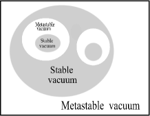
Figure 8: A nested droplets configuration.

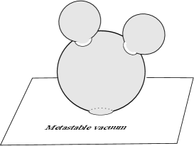
Figure 9: The metric of the nested droplets configuration in presence of gravity.

The Z-Z conjecture formulated above gives a prediction for the subleading term in the small $\zeta$ expansion of ${\cal G}_{\text{low}}$, provided the leading term is known. From (3.25) we find

$$\begin{aligned} {\cal G}_{\text{low}}&={\cal G}_{0}\,+C_{1}\,f+C_{2}\,f^{g_{\text{low}}}+\dots\\ &=\tilde{\cal G}_{0}+\tilde{\cal G}_{1}\ \zeta^{4(p-1)\over 3p-1}+\tilde{\cal G}_{2}\ \zeta^{4p\over 3p-1}+\dots,\end{aligned}$$ (3.33)

with $\tilde{\cal G}<0$. We can develop further the arguments of [22] by taking into account the droplet-inside-droplet configurations as the one shown in Fig. 9. The solution of the Liouville equation for such a nested configuration describes a metric that resembles the surface of a cactus (without the spines), depicted in Fig. 9. It consists of several bubbles of the stable phase connected by thin throats of the metastable phase. The contribution of $n$ droplets within a droplet factorizes into the partition function of a sphere with $n+1$ punctures and $n$ partition functions on a sphere with one puncture. The total power of $|{\cal F}|$ is

$$f^{g_{\text{low}}-n}\left(f^{g_{\text{low}}}\right)^{n}=\zeta^{{4p\over 3p-1}+{4n\over 3p-1}},\quad n=1,2,\dots.$$ (3.34)

In this way the Z-Z conjecture gives not only the subleading term, but also the complete small $\zeta$ expansion of the scaling function ${\cal G}_{\text{low}}$:

$${\cal G}_{\text{low}}(\zeta)=\tilde{\cal G}_{0}+\sum_{n\geq 0}\tilde{\cal G}_{n+1}\ \zeta^{{4(p-1)\over 3p-1}+{4n\over 3p-1}}.$$ (3.35)

The position of the Langer cut is at $\arg\zeta=\pi\alpha_{\rm s}^{\text{low}}=\pi{3p-1\over 4(p-1)}$. When $n>1$ the Langer singularity appears before reaching the negative axis, while for $0<n<1$ it appears after crossing the negative axis.

3.4 The scaling function $\Phi(\eta)$

To study the free energy for a large magnetic field, or equivalently at a small temperature $t$, we introduce the scaling function $\Phi(\eta)$ defined by

$${\cal F}(t,h)=h^{1/\alpha_{\rm s}}\Phi(\eta),\quad\eta=h^{-1/\omega}\ t\,.$$ (3.36)

Depending on the sign of $t$, the new scaling function $\Phi(\eta)$ is related to ${\cal G}_{\text{high}}(\xi)$ or ${\cal G}_{\text{low}}(\zeta)$,

$$\Phi(\eta)=\begin{cases}\eta^{{1/\alpha_{\epsilon}}}\,{\cal G}_{\text{high}}(1/\eta^{\omega})&\quad\text{if }\ t>0\ \text{and}\ h>0,\\ (-\eta)^{{1/\alpha_{\epsilon}}}\,{\cal G}_{\text{low}}(1/(-\eta)^{\omega})&\quad\text{if }\ t<0\ \text{and}\ h>0.\end{cases}$$ (3.37)

As in the flat case, for a given value $h\neq 0$ of the magnetic field, the matter theory has a mass gap and ${\cal F}(t,h)$ should be analytic in $t$. Hence, the scaling function $\Phi(\eta)$ should be analytic in a finite strip containing the real axis. Near $\eta=0$, it is represented by the power series

$$\Phi(\eta)=\Phi_{0}+\Phi_{1}\,\eta+\Phi_{2}\eta^{2}+\dots$$ (3.38)

with finite radius of convergence. According to (3.37), the series expansion of $\Phi(\eta)$ near the origin determines the expansion of ${\cal G}_{\text{high}}(\xi)$ and ${\cal G}_{\text{low}}(\zeta)$ at infinity:

$${\cal G}_{\text{high}}(\xi)=\sum_{j=0}^{\infty}\Phi_{j}\ \xi^{1-j\alpha_{\epsilon}\over\alpha_{\rm s}},\qquad{\cal G}_{\text{low}}(\zeta)=\sum_{j=0}^{\infty}(-1)^{j}\ \Phi_{j}\ \zeta^{1-j\alpha_{\epsilon}\over\alpha_{\rm s}}.$$ (3.39)

The principal sheet of $\Phi(\eta)$ can be split into four sectors as in Fig. 10. The right half-plane $\Re\xi>0,$ where ${\cal G}_{\text{high}}(\xi)$ is analytic, is mapped to the the HT wedge on the principal sheet of $\Phi(\eta)$, defined as

$$\text{HTW:}\qquad|\arg\eta|<{\pi\over 2\omega}={2\pi\over 3p+1}.$$ (3.40)

The two Yang-Lee branch points in the $\xi$ plane correspond to two simple branch points of $\Phi(\eta)$ at

$$\eta^{{}_{{}^{\text{YL}}}}_{\pm}=e^{\pm i\pi/2\omega}\eta_{c},\qquad\eta_{c}=\xi_{c}^{-1/\omega}.$$ (3.41)

To exploit the analyticity of $\Phi(\eta)$ at sufficiently small $\eta$ we place the two YL cuts such that they go to infinity along the rays $\arg(\eta)=\pm{\pi/2\omega}$. Furthermore, the $\zeta$-plane cut along the negative axis, where ${\cal G}_{\text{low}}(\zeta)$ is analytic, maps onto the LT wedge on the principal sheet of $\Phi(\eta)$ defined as

$$\text{LTW:}\qquad|\arg(-\eta)|<{\pi\over\omega}={4\pi\over 3p+1}.$$ (3.42)

The two edges of the Langer cut in the $\zeta$-plane are mapped to the two rays $\arg(-\eta)=\pm{\pi/\omega}$.

Coupling to gravity, or taking the average with respect to geometries, cannot add new singularities to the free energy. Therefore, if the $O_{n}$FT satisfies the extended analyticity, this must be true also for $O_{n}$QG. If this is the case, the function $\Phi(\eta)$ must be analytic in the whole $\eta$ plane with two cuts going from the points (3.41) to infinity, including the ‘shadow domain’ which separates the HT and the LT wedges.

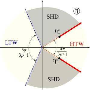
Figure 10: Principal sheet of the $\eta$-plane for the scaling function $\Phi(\eta)$ in presence of gravity. The LT wedge $|\arg(-\eta)|<{4\pi\over 3p+1}$ is the image of the domain of the analyticity of the scaling function ${\cal G}_{\text{low}}(\zeta)$. The HT wedge $|\arg(\eta)|<{2\pi\over 3p+1}$ is the image of the right half plane of the principal sheet of ${\cal G}_{\text{high}}(\xi)$.

4 Analysis of the matrix model explicit solution

In this section we show that the free energy extracted from the exact solution of the discrete model does have the properties claimed in the previous section.

4.1 Lattice formulation on a planar graph

The $O(n)$ loop model can be defined on any trivalent planar graph $\Gamma$. For any value of $n$, the partition function is equal to the sum of all configurations of self- and mutually avoiding loops with activity $n$ and open lines with activity $\vec{H}^{2}$,

$${\cal Z}_{{}_{O(n)}}(T,H;\Gamma)=\sum_{\text{polymers on }\Gamma}\;(1/T)^{\text{total length of the polymers}}\,n^{\#\text{loops}}\,\vec{H}^{2\#\,\text{open lines}}.$$ (4.1)

An example of such a configuration on a graph with the topology of the disk is given in Fig.6.

In the $O(n)$ model on a dynamical lattice, the planar graph $\Gamma$ itself is treated as a statistical object. The partition function of the $O(n)$ model on a dynamical sphere of volume ${N}$ is defined as the average of the partition function (4.1) over all graphs $\Gamma_{N}$ having $N$ vertices and the topology of a sphere,

$$\begin{aligned} {\cal Z}_{N}^{\text{sphere}}(T,\vec{H})&=\sum_{\Gamma_{N}}{\cal Z}_{{}_{O(n)}}(T,\vec{H};\Gamma_{N})\,.\end{aligned}$$ (4.2)

Similarly, the partition function on a dynamical disk of volume $N$ and boundary length $L$ is defined as a sum over all planar graphs $\Gamma_{N,L}$ with $N$ vertices and $L$ external lines, having the topology of a disk,

$$\begin{aligned} {\cal Z}_{N,L}^{\text{disk}}(T,\vec{H})&=\sum_{\Gamma_{N,L}}{\cal Z}_{{}_{O(n)}}(T,\vec{H};\Gamma_{N,L})\,.\end{aligned}$$ (4.3)

The disk partition function above is defined for the simplest boundary condition with no special weight assigned to the boundary spins. This boundary condition means that the loops are repelled from the boundary, as in Fig. 6.

We are going to compute the universal piece of the specific free energy

$${\cal F}(T,\vec{H})\stackrel{{\scriptstyle\text{def}}}{{=}}\lim_{N\to\infty}{\log{\cal Z}_{N}^{\text{sphere}}(T,\vec{H})\over N},$$ (4.4)

as well as the boundary specific free energy

$${\cal F}^{B}(T,\vec{H})\stackrel{{\scriptstyle\text{def}}}{{=}}\lim_{N,L\to\infty}{{\cal Z}_{N,L}^{\text{disk}}(T,\vec{H})-N{\cal F}(T,\vec{H})\over L}.$$ (4.5)

For that it is easier first to evaluate the grand partition functions

$$\begin{aligned} {\cal Z}^{\text{sphere}}(\bar{\mu},T,\vec{H})&=\sum_{{N}=0}^{\infty}e^{-\bar{\mu}{N}}{\cal Z}^{\text{sphere}}_{{N}}(T,\vec{H})\,,\\ {\cal Z}^{\text{disk}}(\bar{\mu},\bar{\mu}_{{}_{\text{B}}},T,\vec{H})&=\sum_{{N}=0}^{\infty}\sum_{L=0}^{\infty}e^{-\bar{\mu}{N}-\bar{\mu}_{{}_{\text{B}}}L}\ {\cal Z}^{\text{disk}}_{{N},L}(T,\vec{H}),\end{aligned}$$ (4.6)

where $\bar{\mu}$ and $\bar{\mu}_{{}_{\text{B}}}$ are the lattice bulk and boundary cosmological constants. The large $N$ and $L$ behavior of the micro-canonical partition functions (4.2) and (4.3) is determined by the behavior of the grand partition functions near the rightmost singularity in $\bar{\mu}$ and $\bar{\mu}_{{}_{\text{B}}}$, which we denote respectively by $\bar{\mu}^{c}$ and $\bar{\mu}_{{}_{\text{B}}}^{c}$.

The universal free energies are determined by the behavior of the partition functions in the vicinity of the critical point $T=T^{c},H=0$, which is parametrized in terms of the renormalized couplings

$$\mu\sim\bar{\mu}-\bar{\mu}^{c},\quad\mu_{{}_{\text{B}}}\sim{\bar{\mu}}_{{}_{\text{B}}}-{\bar{\mu}}_{{}_{\text{B}}}^{c}\,\quad t\sim T-T^{c},\quad h\sim|\vec{H}|.$$ (4.7)

All the information about the universal behavior is contained in the singular parts of the partition functions, which we denote by ${\cal Z}$ and ${\cal U}$,

$$\begin{aligned} {\cal Z}^{\text{sphere}}(\bar{\mu},T,\vec{H})&={\cal Z}^{\text{sphere}}_{\text{reg}}(\bar{\mu},T,\vec{H})+\,{\cal Z}(\mu,t,h),\\ {\cal Z}^{\text{disk}}(\bar{\mu},{\bar{\mu}}_{{}_{\text{B}}},T,\vec{H})&={\cal Z}^{\text{disk}}_{\text{reg}}(\bar{\mu},{\bar{\mu}}_{{}_{\text{B}}},T,\vec{H})+\,{\cal U}(\mu,\mu_{{}_{\text{B}}},t,h)\,.\end{aligned}$$ (4.8)

The regular terms describe degenerate configurations that diverge in the large $N$ limit and should be thrown away in the renormalization process. The renormalized coupling constants $t,h,\mu,\mu_{{}_{\text{B}}}$ can be identified with coupling constants of Sect. 3 up to numerical normalization factors.

4.2 The solution

We give the derivation of the analytic expressions for ${\cal Z}$ and ${\cal U}$ in appendix A. The solution for the disk grand partition function $\mathcal{U}$ is analytic in the boundary coupling $\mu_{{}_{\text{B}}}$ everywhere in the complex plane, except for a branch cut along the interval $[-\infty,-M]$. The function $M=M(\mu,t,h)$ gives the position of the rightmost singularity of ${\cal U}$ in the $\mu_{{}_{\text{B}}}$ complex plane. The renormalized boundary cosmological constant $\mu_{{}_{\text{B}}}$ is defined so that at the critical point $\mu=t=0$ the singularity is placed at the origin: $M(0,0,0)=0$.

The solution can be written conveniently in a hyperbolic parametrization which resolves the branch point at $\mu_{{}_{\text{B}}}=-M$. The boundary coupling $\mu_{{}_{\text{B}}}$ is replaced by a hyperbolic parameter $\tau$, defined as

$$\mu_{{}_{\text{B}}}\ \ =M\cosh(\tau).$$ (4.9)

All the observables must be even functions of $\tau$, and their expression can be written solely in terms of hyperbolic cosines. To shorten the formulas, we introduce the notation

$$C_{a}(\tau)\stackrel{{\scriptstyle\text{def}}}{{=}}{M^{a}\over a}\cosh(a\tau),\qquad a\in{\mathbb{R}}.$$ (4.10)

Then, up to a normalization of the coupling constants and the partition functions, the function $M(\mu,t,h)$ is determined by the transcendental equation

$$\mu=\frac{M^{2}}{2}-t\ \frac{M^{2(1-{1\over p})}}{2(1-{1\over p})}+h^{2}{M^{-(1+{1\over p})}\over 1+{1\over p}},$$ (4.11)

and the derivatives of the disk partition function in $\mu_{{}_{\text{B}}}$ and in $\mu$ are written in the parametric form as

$$\begin{aligned} -{\partial{\cal U}\over\partial\mu_{{}_{\text{B}}}}&=C_{{p+1\over p}}(\tau)+t\,C_{{p-1\over p}}(\tau)+{h^{2}}\ {M^{-{p-1\over p}}C_{{p-1\over p}}(\tau)-M^{-{p+1\over p}}C_{{p+1\over p}}(\tau)\over 2\ [C_{1}(\tau)]^{2}}\\ {\partial{\cal U}\over\partial\mu}&={C_{1/p}(\tau)},\\ \mu_{{}_{\text{B}}}&=C_{1}(\tau).\end{aligned}$$ (4.12)

Finally, the second derivative of the partition function on the sphere is given by

$$u\equiv-\partial_{\mu}^{2}{\cal Z}=M^{{2/p}}.$$ (4.13)

One can eliminate $M$ from (4.11) and (4.13) and write the equation of state for the susceptibility $u=-\partial_{\mu}^{2}{\cal Z}$,

$$\mu={u^{p}\over 2}-t\ {u^{p-1}\over 2(1-{1\over p})}+h^{2}\ {u^{-(p+1)/2}\over 1+{1\over p}}\ .$$ (4.14)

4.3 Microcanonical partition functions and analytic expressions for the bulk and boundary specific free energies

The specific free energy can be extracted from the leading exponential behavior of the micro-canonical partition function when the volume tends to infinity. Knowing the grand canonical partition functions in the thermodynamical limit, we can reconstruct the micro-canonical ones. In this limit, the discrete sums in (4.6) are replaced by integrals with respect to the area $A$ and the length $\ell$:

$$\begin{aligned} {\cal Z}(\mu,t,h)&=\int_{0}^{\infty}dA\,e^{-\mu A}\ {\cal Z}_{A}(t,h)\\ {\cal U}(\mu,\mu_{{}_{\text{B}}},t,h)&=\int_{0}^{\infty}dA\int_{0}^{\infty}d\ell\ e^{-\mu A-\mu_{{}_{\text{B}}}\ell}\ {\cal Z}_{A,\ell}(t,h).\end{aligned}$$ (4.15)

The partition functions for a given area and length are computed by taking the inverse Laplace transforms. With this definition the regular part of the specific free energy is automatically subtracted.

For the partition function on the sphere, ${\cal Z}_{A}$, we find, after integrating by parts,

$${\cal Z}_{A}(t,h) = {1\over A^{2}}\int{d\mu\over 2\pi i}\ e^{\mu A}\ \partial_{\mu}^{2}{\cal Z}(t,\mu,h)$$ (4.16)

$$= {1\over A^{3}}\int{du\over 2\pi i}\,\ e^{\mu(u)A}\ ,$$

where $\mu(u)$ is given by (4.14). The integral over $\mu$ goes along a contour going upwards and having all the singularities of $\partial_{\mu}^{2}{\cal Z}$ on the left. The large $A$ asymptotics, given by the contribution of the saddle point, is

$${\cal Z}_{A}(t,h)\sim A^{-3-1/2}\ e^{-{\cal F}(t,h)\,A},$$ (4.17)

where ${\cal F}(t,h)$ is by definition the specific free energy, evaluated by the saddle point condition

$${\cal F}(t,h)=-\mu(y),\quad(\partial\mu/\partial u)_{u=y}=0.$$ (4.18)

The exponent for the power in the saddle-point result (4.17) corresponds to a pure gravity theory ($c_{\text{matter}}=0$). This is because the asymptotic is evaluated for values of the area and the length much larger than the correlation volume of the $O(n)$ spins, $A_{\text{cor}}=1/{\cal F}(t,h)$.

In a similar way, the micro-canonical partition function on the disk ${\cal Z}_{A,\ell}$ is given by a double integral in $\mu$ and $\mu_{{}_{\text{B}}}$. The large $\ell$ asymptotics is determined by the rightmost singularity of ${\cal U}$ in the $\mu_{{}_{\text{B}}}$ plane, which is the branch point at $\mu_{{}_{\text{B}}}=-M$. This gives for the boundary free energy

$${{{\cal F}}_{\text{B}}}(t,h)=y^{p/2},\quad(\partial\mu/\partial u)_{u=y}=0.$$ (4.19)

The bulk and the boundary specific free energies are intensive characteristics of the system and as such do not depend on the global properties of the random surface such as the number of handles or boundaries.

From the equation of state (4.14) one obtains the analytic expressions for the specific free energies,

$$\begin{aligned} {\cal F}(t,h)=&-{y^{p}\over 2}+t\,{y^{p-1}\over 2(1-{1\over p})}-h^{2}\,{y^{-(p+1)/2}\over 1+{1\over p}}\\ =&-\frac{1}{2}y^{p-1}\left(\frac{3p+1}{p+1}y-\frac{p(3p-1)}{p^{2}-1}t\right),\\ {{{\cal F}}_{\text{B}}}(t,h)=&\ \ \ \ y^{p/2},\end{aligned}$$ (4.20)

where the saddle point value $u=y$ is the solution of

$$y^{(3p-1)/2}(y-\,t)=h^{2}.$$ (4.21)

4.4 The scaling functions ${\cal G}_{\text{high}}(\xi)$ and ${\cal G}_{\text{low}}(\zeta)$

Let us first analyze the scaling function for the HT regime ($t>0$), defined by (3.15),

$${\cal F}(t,h)=t^{p}\,{{\cal G}}_{\text{high}}(\xi),\quad\xi=h\,t^{-({3p+{1})/4}}.$$ (4.22)

By (4.20) and (4.21) the scaling function is given in a parametric form by

$$\begin{aligned} {{\cal G}}_{\text{high}}&=\frac{1}{2}y^{p-1}\left(\frac{p(3p-1)}{p^{2}-1}-\frac{3p+1}{p+1}y\right)\\ \xi^{2}\quad&=y^{(3p-1)/2}\ \left(y-1\right)\,.\end{aligned}$$ (4.23)

The solution can be expanded (see Appendix B) in a Taylor series in $\xi^{2}$,

$${\cal G}_{\text{high}}(\xi)=\frac{p}{2}\sum_{n=0}^{\infty}{\dfrac{\Gamma\left[\frac{3p+1}{2}n-p\right]}{\Gamma\left[\frac{3p-1}{2}n+2-p\right]}{(-\xi^{2})^{n}\over n!}}\simeq\dfrac{1}{2(p-1)}-\dfrac{p}{p+1}\xi^{2}+\cdots$$ (4.24)

The expansion is convergent in the circle $|\xi|<\xi_{c}$, where

$$\xi_{c}=\,\textstyle{\sqrt{2}\ {(3p-1)^{3p-1\over 4}\over(3p+1)^{3p+1\over 4}}}$$ (4.25)

is determined by the position of the nearest singularity $d\xi/dy=0$. The function $y(\xi)$ has in general an infinite number of branch points, all at distance $\xi_{c}$ from the origin,

$$\xi_{k,\pm}=\pm i\,e^{i\pi k{3p+1\over 2}}\xi_{c},\quad k\in{\mathbb{Z}}.$$ (4.26)

The two branch points on the physical sheet, $\xi_{\pm}^{{}_{{}^{\text{YL}}}}=\xi_{0,\pm}=\pm i\xi_{c}$, are of course the positions of the two YL singularities. Near the Yang-Lee branch points the scaling function has the expected behavior of the YL model coupled to gravity, eq. (3.18).

Looking at the integral representation (4.16), it is easy to see that the YL edges appear as the result of condensation of zeroes of the microcanonical partition function ${\cal Z}_{A}(t,h)$. When $\xi$ is close to $\xi_{+}^{{}_{{}^{\text{YL}}}}$ or to $\xi_{-}^{{}_{{}^{\text{YL}}}}$, the second derivative $\mu^{\prime\prime}(u)$ vanishes at the saddle point together with $\mu^{\prime}(u)$ and the integral is approximated by Airy integral. When $|\xi|<\xi_{c}$, the fixed area partition function has no zeroes and the power $3/2$ singularity of ${{\cal G}}_{\text{high}}(\xi)$ reflects the asymptotics of the Airy function for large positive values of the argument. On the other hand, when $\xi$ is purely imaginary and $|\xi|>\xi_{c}$, the product of the Airy functions associated with $\xi_{+}^{{}_{{}^{\text{YL}}}}$ and $\xi_{-}^{{}_{{}^{\text{YL}}}}$ has zeroes with density

$$\rho\sim A^{1/3}\sqrt{\xi^{2}+\xi_{c}^{2}},$$ (4.27)

which condense into the two YL cuts.

We saw that the scaling function ${{\cal G}}_{\text{high}}(\xi)$ has the analytic properties anticipated in Sect. 3.2, for which there was little doubt. Now let us turn to the scaling function ${{\cal G}}_{\text{low}}(\zeta)$, whose analytical properties were the subject of the speculations of Sect. 3.3.

The scaling function ${{\cal G}}_{\text{low}}(\zeta)$ for the LT regime ($t<0$), defined by (3.15),

$${\cal F}(t,h)=(-t)^{p}\,{{\cal G}}_{\text{low}}(\zeta),\quad\zeta=h\ (-t)^{-({3p+{1})/4}},$$ (4.28)

is written in parametric form as

$$\begin{aligned} {{\cal G}}_{\text{low}}\ &=-\frac{1}{2}y^{p-1}\left(\frac{p(3p-1)}{p^{2}-1}+\frac{3p+1}{p+1}y\right)\,,\\ \zeta^{2}\quad&=\ y^{(3p-1)/2}\ \left(y+1\right)\,.\end{aligned}$$ (4.29)

The asymptotics for small and large positive $\zeta$ have the form anticipated in Sect. 3.3,

$${{\cal G}}_{\text{low}}(\zeta)=\begin{cases}\ \zeta^{{4p\over 3p+1}}&\text{ if }\ \zeta\to\infty,\\ \zeta^{{4(p-1)\over 3p-1}}&\text{if }\ \zeta\to 0\,.\\ \end{cases}$$ (4.30)

On the principal sheet, the cut relating the branch points at $\zeta=0$ and $\zeta=\infty$ is placed on the negative real axis. The small $\zeta$ expansion of the bulk free energy is computed in Appendix B. It is indeed of the form (3.35),

$${\cal G}_{\text{low}}(\zeta) =-{p(3p-1)\over 2(p^{2}-1)}\zeta^{\frac{4(p-1)}{3p-1}}+{1\over 2}\zeta^{\frac{4(p-1)}{3p-1}+\frac{4}{3p-1}}+{p\over 2(3p-1)}\zeta^{\frac{4(p-1)}{3p-1}+\frac{8}{3p-1}}+\dots\ .$$ (4.31)

The coefficient $\tilde{\cal G}_{n}$ of the series are given by

$$\tilde{\cal G}_{0}=0\,;\qquad\tilde{\cal G}_{n}={1\over n!}\ \dfrac{p}{3p-1}\ {\dfrac{\Gamma\left[\frac{3p+1}{3p-1}n-\frac{p+1}{3p-1}\right]}{\Gamma\left[\frac{2}{3p-1}n+\frac{5p-3}{3p-1}\right]}}\qquad(n\geq 1).$$ (4.32)

The vanishing constant term reflects our convention for the integration constant in the derivation of the transcendental equation for $\mu$ in Appendix A.2. A non-zero constant term is generated by a redefinition of the cosmological constant $\mu\to\mu+c|t|^{p}$.

4.5 The scaling function $\Phi(\eta)$

Here we analyze the scaling function $\Phi(\eta)$ defined by (3.36),

$${\cal F}(t,h)=h^{{4p\over 3p+1}}\,\Phi(\eta),\quad\eta=t\,h^{-{4\over 3p+1}}.$$ (4.33)

Using (4.20) and (4.21) we write the parametric representation of $\Phi(\eta)$,

$$\begin{aligned} \Phi&={\textstyle{1\over 2}}\textstyle{{p(3p-1)\over p^{2}-1}}\ v^{-{p+1\over 2}}-{\textstyle{1\over 2}}\textstyle{{2p-1\over p-1}}\ v^{p}\\ \eta&=v-v^{-{3p-1\over 2}}\,.\end{aligned}$$ (4.34)

The function $\Phi(\eta)$ is analytic inside the disk

$$|\eta|<\eta_{c},\qquad\eta_{c}=\xi_{c}^{-1/\omega}=\textstyle{{3p+1\over 2}\left({3p-1\over 2}\right)^{-{3p-1\over 3p+1}}},$$ (4.35)

where it is given by the power series (3.38). For the coefficients $\Phi_{n}$ we find (Appendix B)

$$\Phi_{0} =-\dfrac{3p+1}{2(p+1)}\,;\qquad\Phi_{n}=\dfrac{p}{3p+1}{(-1)^{n}\over n!}{\dfrac{\Gamma\left[\frac{2n}{3p+1}-\frac{2p}{3p+1}\right]}{\Gamma\left[\frac{4p+2}{3p+1}-\frac{3p-1}{3p+1}n\right]}}\qquad(n\geq 1).$$ (4.36)

For general $p$ the function $\Phi(\eta)$ has an infinite number of simple branch points, the solutions of the equation $dv/d\eta=0$,

$$\eta_{j}=e^{2\pi i{2j-1\over 3p+1}}\ \eta_{c},\qquad j\in{\mathbb{Z}}.$$ (4.37)

There are no other singularities at finite $\eta$. The cuts starting at $\eta_{j}$ go along the radial direction and end at the branch point at $\eta=\infty$, which is in general of infinite order. The principal sheet has two branch points, $\eta^{{}_{{}^{\text{YL}}}}_{+}=\eta_{0}$ and $\eta^{{}_{{}^{\text{YL}}}}_{-}=\eta_{1}$, which are the images of the YL branch points in the $\xi$ plane, as shown in Fig. 10. The two branch cuts separate the sectors HTW and LTW$\cup$SHD defined in Sect. 3.4, in which the scaling function has different asymptotics,

$$\Phi(\eta) \sim \begin{cases}\ -\ \eta^{p}&\text{ if }\ \ \eta\to\infty,\ \eta\in\text{HTW},\\ -(-\eta)^{p+1\over 3p-1}&\ \text{if }\ \eta\to\infty,\ \eta\in\text{LTW}\cup\text{SHD}\,.\\ \end{cases}$$ (4.38)

According to (4.34), the Riemann surface of $\Phi(\eta)$ is symmetric under a rotation at angle ${4\pi\over 3p+1}$. Therefore all sheets are rotated images of the principal sheet. Let us label the sheets by the integers $\dots,S_{-1},S_{0},S_{1},\dots$, where $S_{0}$ is the principal sheet. Then the sheet $S_{k}$ has two cuts going in the radial direction and starting at the points $\eta_{k}$ and $\eta_{k+1}$. For irrational $p$, the Riemann surface has an infinite number of auxiliary sheets.

Let us now consider the case when $p=2m-1$ is odd integer, when the matter QFT is a perturbation of a unitary CFT. The Riemann surface of $\Phi(\eta)$ has ${3p+1\over 2}=3m-1$ sheets and $3m-1$ simple branch points $\eta_{0},\dots,\eta_{3m-2}$. At infinity, the $3m-1$ cuts join in a ramification point of order $3m-2$ where $\Phi\sim\eta^{m/(3m-2)}$. If we cut all sheets along a circle with radius larger $\eta_{c}$, the exterior part of the Riemann surface will split into $2$ disconnected pieces as shown in Fig. 11. When analytically continuing from the HTW, one returns to the principal sheet after circling once the origin. When analytically continuing from the LTW, one should circle $3m-2$ times around the origin in order to return to the principal sheet.

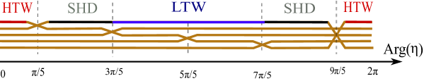
Figure 11: A circular slice of the Riemann surface of $\Phi(\eta)$ for $m=2$ $(p=3)$.

4.6 The complex curve of the specific free energy

The two scaling functions were obtained by eliminating $y$ from the two equations (4.20) and (4.21), assuming that the temperature coupling is positive or negative. The equations allow to consider the coupling constants $t$ and $h$ as non-restricted complex variables and define the scaling functions in the HT and the LT regimes as the restrictions to two different sheets of the same analytic function ${\cal G}(\xi)$, defined by (4.23),

$$\begin{aligned} {\cal G}\,&={\textstyle{1\over 2}}\textstyle{p(3p-1)\over p^{2}-1}\,y^{p-1}-{\textstyle{1\over 2}}\textstyle{3p+1\over p+1}\,y^{p}\\ \xi^{2}&=y^{(3p-1)/2}\ \left(y-1\right)\,.\end{aligned}$$ (4.39)

In this sense one can speak of the complex curve of the specific free energy. When $p$ and $2\omega={3p+1\over 2}$ are integers, this is an algebraic curve of genus zero.

The scaling function ${\cal G}_{\text{high}}(\xi)$ is the restriction of ${\cal G}(\xi)$ on the principal (HT) sheet, while the scaling function ${\cal G}^{\text{low}}$ is obtained as the analytic continuation of ${\cal G}_{\text{high}}(\zeta)$ below the YL cuts,

$$\begin{aligned} {\cal G}_{\text{high}}(\xi)&={\cal G}(\xi),\qquad\qquad\qquad\qquad\qquad\xi\in\text{ HT sheet},\\ \qquad{{\cal G}}_{\text{low}}(\zeta)&=e^{\mp i\pi p}\,{{\cal G}}_{\text{high}}(e^{\pm i\pi{3p+1\over 4}}\zeta),\ \qquad\zeta=e^{\mp i\pi\textstyle{3p+1\over 4}}\xi\in\text{LT sheet}.\end{aligned}$$ (4.40)

Let us first remind the structure of the Riemann surface of ${\cal G}(\zeta)$ in the simplest case of the Ising model, which has been analyzed in the unpublished work by Al. Zamolodchikov [21]. When $p=3$, the Riemann surface represents a five-sheet cover of the complex $\xi$-plane. The five sheets of the Riemann surface of the curve $\xi^{2}=y^{5}-y^{4}$ are shown in Fig.12. There are two copies of the LT sheet, each of then connected to the HT sheet by an auxiliary sheet having two cuts. After changing the variable $\xi\to\zeta=e^{\mp i5\pi/4}\xi$, the Langer cut in the two copies of the LT sheet places itself on the negative axis in the $\zeta$-plane.

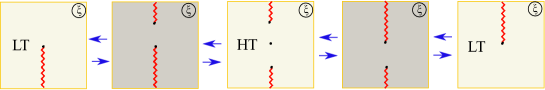
Figure 12: The five sheets of the Riemann surface for the Ising model, $p=3$.

For general $p$ the analytic continuation from the HT sheet can be performed in four different ways, by going in clockwise/anticlockwise direction beneath the upper/lower YL cut. That is, the HT sheet is connected in general to four different copies of the LT sheet, which form an orbit of the $Z_{2}\times Z_{2}$ symmetry (1.22) of the meromorphic function ${\cal G}(\xi)$. This symmetry preserves the HT sheet (or each of the copies of the HT sheet, if there are several of them), but not the LT sheets.

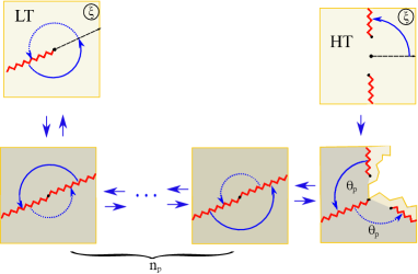
Figure 13: Analytic continuation under the YL cut from the HT sheet to the LT sheet.

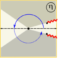
Figure 14: Analytic continuation under the YL cut from the HT sheet to the LT sheet.

In Fig.14 we show the part of the Riemann surface containing a path, starting from the real axis on the HT sheet, going under the upper YL cut and continuing anti-clockwise, until it reaches the positive axis ($\zeta\equiv e^{i\pi{3p+1\over 4}}\xi>0$) of the LT sheet. For convenience we place the Langer cut on the negative $\zeta$-axis of the LT sheet. The total angle swept by the path is $\omega\pi={3p+1\over 4}\pi$. We taylor the sheets of the Riemann surface visited by the path according to the following decomposition of the angular distance along the path,

$$\textstyle{3p+1\over 4}\pi={\textstyle{1\over 2}}\pi+\theta_{p}+n_{p}\pi+\pi\,,\qquad(n_{p}\ \text{ integer},\ \ 0<\theta_{p}\leq\pi).$$ (4.41)

This means that the second sheet has, besides the YL cut, a cut along the ray $\arg(\xi)={\textstyle{1\over 2}}\pi+\theta_{p}$, and possibly other cuts. The remaining $n_{p}$ identical sheets have two cuts along the rays $\arg(\xi)={\textstyle{1\over 2}}\pi+\theta_{p}$ and $\arg(\xi)={\textstyle{1\over 2}}\pi+\theta_{p}+\pi$. The axis $\zeta>0$ of the LT sheet is rotated with respect to the positive axis of the $\xi$-plane at angle ${\pi\over 2}+\theta_{p}$ if $n_{p}$ is odd, and ${\pi\over 2}+\theta_{p}+\pi$ if $n_{p}$ is even. The image of the path in the $\eta$-plane starts at the positive axis and ends at the negative axis, staying all the time in the upper half of the principal sheet of the function $\Phi(\eta)$, as shown in Fig.14. If the path is continued further anti-clockwise (the punctured line), it will visit once again the $n_{p}$ sheets and then the second sheet, to reach (in general another copy of) the HT sheet. The image of the path in the $\eta$-plane returns to the positive axis.

If one continues in the same way, the same pattern will reappear, rotated at angle $2\theta_{p}$, and so on. The symmetry $\xi\to e^{2i\theta_{p}}\xi$ of the Riemann surface of ${\cal G}(\xi)$ reflects the symmetry $\eta\to e^{2i\pi}\eta$ of the Riemann surface of $\Phi(\eta)$. For rational values of $p$, the path will eventually return to the starting point after a finite number of turns around the origin.

Let us consider some particular cases.

$\bullet$ Polymers ($n=0,\ p=2$).

The partition function is that of a grand canonical ensemble of open linear polymers. The Riemann surface for curve $\xi^{2}=y^{7/2}-y^{5/2}$ has 7 sheets, depicted in Fig.15. There are two copies of the HT sheet and four copies of the LT sheet. There is only one connecting sheet on which the function $y(\xi)$ has four simple branch points at $\pm\xi_{c},\pm i\xi_{c}$, as well as at $\xi=0$ and $\xi=\infty$.

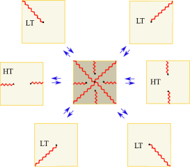
Figure 15: The seven sheets of the Riemann surface for linear polymers, $p=2$ ($n_{p}=0$).

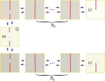
Figure 16: The Riemann surface for $p=2m-1$ with $m$ even. Here $n_{p}={3\over 2}m-3$, $\theta_{p}=\pi$.

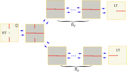
Figure 17: Riemann surface for $p=2m-1$ with $m$ odd. Here $n_{p}={3m-5\over 2}$, $\theta_{p}={\textstyle{1\over 2}}\pi$.

$\bullet$ $p=2m-1,\quad m\in{\mathbb{N}}$.

In this case the critical theory is a unitary CFT and the operator coupled to the magnetic field is the primary field $\Phi_{m,m}$. When $p$ is odd integer, the equations (4.39) become algebraic. The function ${\cal G}(\xi)$ has, apart of $\xi=0$ and $\xi=\infty$, only two branch points, $\xi=\pm i\xi_{c}$. The Riemann surface has $3m-1$ sheets, which include one HT sheet and two copies of the LT sheet. The $3m-1$ sheets of the Riemann surface are shown in Fig.17, for $m$ even, and in Fig.17, for $m$ odd. In the first case $n_{p}={3\over 2}m-3$ and $\theta_{p}=\pi$, while in the second case $n_{p}={3m-5\over 2}$ and $\theta_{p}={\textstyle{1\over 2}}\pi$.

Appendix A Matrix model solution for $O(n)$ spin system in magnetic field

A.1 Mapping to a matrix model and loop equation for the resolvent

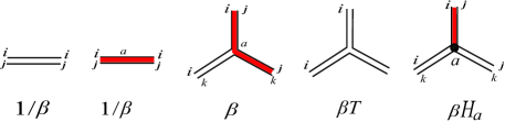
Figure 18: Feynman rules for the $O(n)$ matrix model in the presence of a magnetic field. The magnetic term $\vec{H}\cdot\vec{\bf Y}$ can be seen as a source for tadpoles.

The $O(n)$ matrix model [23], with an extra term taking into account the magnetic field, is the zero-dimensional planar field theory whose Feynman graphs are built according to the Feynman rules shown in Fig.(18). The partition function of the matrix model represents the integral over one hermitian matrix ${\bf M}$ and a $O(n)$ vector $\vec{\bf Y}$ whose components are hermitian matrices,

$${Z}_{N}\sim\int d{\bf M}\,d^{n}{\bf Y}e^{\beta{\rm tr}[-{1\over 2}{\rm Tr}{\bf M}^{2}-{1\over 2}{\rm Tr}\vec{\bf Y}^{2}+{T\over 3}{\bf M}^{3}+{1\over 2}{\bf M}\vec{\bf Y}^{2}+\vec{H}\cdot\vec{\bf Y}]}\,,$$ (A.1)

At this stage the number $n$ is considered integer. Expanding the free energy of the matrix model as a sum over Feynman diagrams, we obtain a sum over all polymer configurations on the disk as the one shown in figure 6. The weight of these diagrams is given by

$$N^{2-2g}\,\left(\dfrac{\beta}{N}\right)^{-\#\text{vertices}/2}\,T^{-L_{\rm tot}}\,n^{\#\text{loops}}\,H^{2\#\,\text{open lines}},$$ (A.2)

where $N$ is the size of the matrices and $g$ is the genus of the ‘fat’ planar graph. The functions defined in (4.6) are expressed in terms of the matrix model as

$$\begin{aligned} {\cal Z}^{\text{sphere}}(\bar{\mu},T,H)&=\lim_{N,\beta\to\infty}\dfrac{1}{N^{2}}\log Z_{N},\\ \ {\cal Z}^{\text{disk}}(\bar{\mu},{\bar{\mu}}_{{}_{\text{B}}},T,H)&=\lim_{N,\beta\to\infty}\dfrac{1}{N^{2}}\left\langle\,{\rm Tr}\log\left(1-e^{-{\bar{\mu}}_{{}_{\text{B}}}}{\bf M}\right)\,\right\rangle,\qquad\beta/{N}=e^{2\bar{\mu}}~{}~{}\text{fixed}.\end{aligned}$$ (A.3)

It is useful to shift the matrix variable as ${\bf M}={\bf X}+{1\over 2}{\bf I}$. Integrating over ${\vec{\bf Y}}$, we write the partition function (A.1) as an integral over the eigenvalues of ${\bf X}$,

$${Z}_{N} \sim \int\prod_{i=1}^{N}{dx_{i}\over(2x_{i})^{n/2}}\,e^{-\beta V(x_{i})}\prod_{i<j}{(x_{i}-x_{j})^{2}\over(x_{i}+x_{j})^{n}}.$$ (A.4)

with (after rescaling of $H$)

$$V(x)=-\frac{T}{3}\Big{(}x+\tfrac{1}{2}\Big{)}^{3}+\frac{1}{2}\Big{(}x+\tfrac{1}{2}\Big{)}^{2}+{H^{2}\over x}.$$ (A.5)

The basic observable in the matrix theory, the resolvent

$$W(x)=\frac{1}{\beta}\left\langle\text{tr}\frac{1}{x-{\bf X}}\right\rangle,$$ (A.6)

is equal, by (A.3), to the derivative of the disk partition function with respect to the boundary cosmological constant. One can check that the critical value of the later is $e^{\mu_{{}_{\text{B}}}}=1/2$, so that the spectral parameter $x$ in (A.6) is equal, up to a normalization, to the renormalized boundary cosmological constant, $x=\mu_{{}_{\text{B}}}$.

The resolvent $W(x)$ splits into a singular part $w(x)$ having a branch cut on the real axis, and an analytic part $W_{\rm reg}(x)$:

$$W(x)\stackrel{{\scriptstyle\text{def}}}{{=}}W_{\rm reg}(x)+w(x)\,.$$ (A.7)

The singular part of $W$ is proportional to the derivative of the disk free energy in the continuum limit ${\cal U}(\mu_{{}_{\text{B}}})$, defined (4.8),

$$w(x)=-{\cal U}^{\prime}(x).$$ (A.8)

The regular part is given by

$$W_{\rm reg}(x) = \frac{2V^{\prime}(x)-nV^{\prime}(-x)}{4-n^{2}}=-{H^{2}\over(2+n)\,x^{2}}-a_{0}-a_{1}x-a_{2}x^{2}.$$ (A.9)

The function $w(x)$ satisfies a quadratic identity that can be obtained using either the loop equation technique or the saddle point approach,

$${w^{2}(x)+w^{2}(-x)+nw(x)w(-x)\over 4-n^{2}}=c_{-4}\,x^{-4}+c_{-2}\,x^{-2}+c_{0}+c_{2}x^{2}+c_{4}x^{4}\,.$$ (A.10)

The coefficients $c_{k}$ are functions of $T$, $\bar{\mu},H$, $W_{1}=\beta^{-1}\langle\text{tr}X\rangle$, $W_{-1}=\beta^{-1}\langle{\rm tr}X^{-1}\rangle$ and $W_{-2}=\beta^{-1}\langle{\rm tr}X^{-2}\rangle$ and can be evaluated from the large-$x$ and small-$x$ asymptotics

$$w(x) = a_{2}x^{2}+a_{1}x+a_{0}+\frac{e^{2\bar{\mu}}}{x}+\frac{W_{1}}{x^{2}}+\frac{H^{2}}{(2+n)x^{2}}+O(x^{-3}),\qquad x\to\infty$$

$$w(x) = {b_{0}\over x^{2}}-W_{-1}-W_{-2}\,x+a_{1}x+O(x^{2}),\qquad x\to 0$$ (A.11)

in (A.10). Obviously

$$c_{-4}={b_{0}^{2}\over 2-n},\quad b_{0}={H^{2}\over 2+n}.$$ (A.12)

The solution of the loop equation (A.10) with the asymptotic (A.1) is given by a meromorphic function with a single cut $[a,b]$ on the first sheet, with $a<b<0$. The coefficient $c_{-4}$ is proportional to $H^{4}$, $c_{2}$ depends only on $T$ and $c_{4}$ is a constant. The coefficients, $c_{-2}$ and $c_{0}$ depend on $T$, $\bar{\mu},H$ directly and through the unknown quantities $W_{1}$, $W_{-1}$ and $W_{-2}$. Fortunately, we do not need to compute these coefficients explicitly in order to find the solution in the scaling limit, as we will see in the next section.

A.2 Solution in the scaling limit

We will solve the loop equation in the vicinity of the double singularity $T=T_{\text{crit}},\ H=0$ and $x=0,\ \bar{\mu}=\bar{\mu}^{c}$. This vicinity is parametrized by the renormalized couplings $t\sim T-T_{\text{crit}},\ h\sim H$ and $\mu_{B}\sim x,\ \mu\sim\bar{\mu}-\bar{\mu}_{c}$. We will use the parametrization (1.9) of the dimensionality $n$, with $1/p=\theta$:

$$n=2\cos(\pi\theta),\quad\theta={1/p}.$$ (A.13)

We will choose a specific normalization of the solution which simplify the formulas. We normalize $t$ and $h$ in such a way that the constants $b_{0}$ and $c_{2}$ are given by

$$b_{0}={\sqrt{2-n}\over 2(1-\theta)}h^{2},\quad c_{2}=\frac{1+\theta}{1-\theta}t.$$ (A.14)

Here we used the fact that $c_{2}$ depends only on $T$.Once this normalization is fixed, the quadratic identity (A.10) determines the solution uniquely.

In the continuum limit, the left bound of the interval supporting the eigenvalue density is sent to $-\infty$, and we can use an hyperbolic parametrization to resolve the branch cut of the resolvent on $[-\infty,-M]$,

$$\mu_{{}_{\text{B}}}\equiv x=M\cosh\tau\,.$$ (A.15)

The solution will be expressed in terms of the functions

$$C_{a}(\tau)={M^{a}\over a}\cosh(a\tau),\qquad a=k\pm\theta,\ \ k=\text{odd integer},$$ (A.16)

which form a complete set in the space of functions having the required analytic properties. In particular they satisfy the shift equation

$$C_{\nu}(\tau+i\pi)+C_{\nu}(\tau-i\pi)+nC_{\nu}(\tau)=0$$ (A.17)

also obeyed by the resolvent $w(\tau)$. Note also that the parametrization (A.15) can be written as $x=C_{1}(\tau)$. In terms of the parameter $\tau$, the functional equation (A.10) becomes a shift equation for the entire function $w(\tau)\equiv w[\mu_{B}(\tau)]$:

$${w^{2}(\tau+i\pi)+w^{2}(\tau)+n\,w(\tau+i\pi)w(\tau)\over 4\sin^{2}(\pi\theta)}={c_{-4}\over[C_{1}(\tau)]^{4}}+{c_{-2}\over[C_{1}(\tau)]^{2}}+c_{0}+c_{2}\,[C_{1}(\tau)]^{2}.$$ (A.18)

It is noted that the term proportional to $c_{4}$ is dropped in the renormalization process.

From the scaling dimension of the resolvent, $w\sim\mu^{(1+\theta)/2}$ (by definition $\mu$ has scaling dimension $1$) it follows that the r.h.s scales as $\mu^{1+\theta}$. From here, one finds the scaling of the coefficients:

$$h\sim\mu^{3+\theta\over 4},\quad t\sim\mu^{\theta},\quad c_{0}\sim\mu^{1+\theta},\quad c_{-2}\sim\mu^{2+\theta}.$$ (A.19)

We will try to satisfy the functional equation (A.18) by the following ansatz,

$$w(\tau) = C_{1+\theta}(\tau)+t\,C_{1-\theta}(\tau)+h^{2}{b_{+}C_{1+\theta}(\tau)+b_{-}C_{1-\theta}(\tau)\over[C_{1}(\tau)]^{2}}$$ (A.20)

The coefficients $b_{\pm}$ are fixed by the two leading terms in the small $x$ behavior (A.1), which can be transposed into conditions on $w(\tau)$ near the point $\tau=\pm i\pi/2$,

$$b_{\pm}=\mp\frac{1}{2}M^{-(1\pm\theta)}.$$ (A.21)

For this solution the coefficients $c_{-2}$ and $c_{0}$ are

$$\begin{aligned} &c_{-2}=-\frac{h^{2}}{4(1-\theta^{2})}\left[h^{2}M^{-2}+{2\over 1+\theta}M^{1+\theta}-{2\over 1-\theta}\,t\,M^{1-\theta}\right]\ ,\\ &c_{0}=\dfrac{1}{4}M^{2+2\theta}+{1\over 2(1-\theta^{2})}\left(h^{2}M^{-1+\theta}(1-t\,M^{-2\theta})-tM^{2}\right)+\dfrac{1}{4}\dfrac{1}{(1-\theta)^{2}}\,t^{2}M^{2-2\theta}.\end{aligned}$$ (A.22)

where $M=M(\mu,t,h)$.

We cannot determine the function $M(\mu,t,h)$ by comparing (A.22) with the r.h.s. of (A.10), because the information about the behavior at large $x$ is lost after taking the continuum limit. Instead, we will make use of the fact that the derivative $\partial_{\mu}w(x)$ does not depend on the potential and have, up to a normalization, a standard form [40]

$$\partial_{\mu}w(x)=-M^{-1+\theta}\ {\sinh\theta\tau\over\sinh\tau}.$$ (A.23)

Comparing this expression with the derivative of the solution (A.20) with respect to $\mu$ at fixed $x$,

$$\partial_{\mu}w|_{x}=-\partial_{\mu}M\left(M^{\theta}-tM^{-\theta}-h^{2}\,M^{-3}\right)\frac{\sinh\theta\tau}{\sinh\tau},$$ (A.24)

yields a compatibility condition, which can be written, after integration, as a transcendental equation for $M$:

$$\mu=\frac{M^{2}}{2}-t\ \frac{M^{2-2\theta}}{2-2\theta}+h^{2}{M^{-1-\theta}\over 1+\theta}.$$ (A.25)

The cosmological constant is determined up to an arbitrary integration constant $\sim t^{1/\theta}$.

The loop mass $M$ is proportional to the second second derivative $u=-\partial_{\mu}^{2}{\cal Z}$ of the partition function on the sphere in the continuum limit, defined in (4.8). There is a simple heuristic argument to see that. The derivative $-\partial_{\mu}{\cal U}(\mu_{{}_{\text{B}}})$ is the partition function on the disk with one marked point in the bulk. In the limit $\mu_{{}_{\text{B}}}\to\infty$ the boundary length vanishes and the boundary can be replaced by a point. The leading term in the limit $\mu_{{}_{\text{B}}}\to\infty$ is therefore proportional to the second derivative $\partial_{\mu}^{2}{\cal Z}$. Expanding at $\mu_{B}\to\infty$ we find

$$-\partial_{\mu}{\cal U}\sim-\mu_{{}_{\text{B}}}^{\theta}+M^{2\theta}\,\mu_{{}_{\text{B}}}^{-\theta}+\text{ lower powers of }\mu_{{}_{\text{B}}}$$ (A.26)

(the numerical coefficients are omitted). We conclude that the second derivative of the sphere partition function is

$$u\equiv-\partial_{\mu}^{2}{\cal Z}=M^{2\theta}.$$ (A.27)

Now we can write the equation of state for the $O(n)$ model on the sphere in its final form

$$\mu={u^{1\over\theta}\over 2}-t\,{u^{{1-\theta\over\theta}}\over 2-2\theta}+h^{2}\ {u^{-{1+\theta\over 2\theta}}\over 1+\theta},\quad u=-\partial_{\mu}^{2}{\cal Z}.$$ (A.28)

Of course, this equation implies certain normalization of $\mu$ and $\mu_{{}_{\text{B}}}$.

Appendix B Series expansions of the scaling functions

We have to deal with the transcendental equations of the form

$$\mu=z+\lambda\,z^{\alpha},\quad\alpha>1.$$ (B.1)

The solution of this equation as a power series can be derived using the Lagrange inversion theorem,

$$z^{\gamma} =\gamma\sum_{n=0}^{\infty}{\dfrac{(-1)^{n}\lambda^{n}}{n!}\dfrac{\Gamma[\alpha n+\gamma]}{\Gamma[(\alpha-1)n+\gamma+1]}\ \mu^{\gamma+n(\alpha-1)}}$$ (B.2)

$$=\mu^{\gamma}-\gamma\ \lambda\mu^{\gamma+\alpha-1}+{\gamma(2\alpha-1+\gamma)\over 2}\ \lambda^{2}\mu^{\gamma+2(\alpha-1)}+\dots.$$

HT expansion:

We would like to find the series expansion in $\xi$ of ${\cal G}_{\text{high}}$, defined by the eq. (4.23). It is easier to first consider the derivative

$$\dfrac{d{\cal G}_{\text{high}}}{d\xi^{2}}=-\dfrac{p}{p+1}\ y^{-(p+1)/2},\quad\xi^{2}=y^{(3p+1)/2}-y^{(3p-1)/2}.$$ (B.3)

After changing the variable to $y=1+f$, we write these equations as

$$\xi^{\frac{2(p+1)}{3p-1}}\dfrac{d{\cal G}_{\text{high}}}{d\xi^{2}}=-\dfrac{p}{p+1}f^{\frac{p+1}{3p-1}},\quad\xi^{\frac{4}{3p-1}}=f^{\frac{2}{3p-1}}+f^{\frac{3p+1}{3p-1}}.$$ (B.4)

We can now use the result (B.2) with $\mu=\xi^{\frac{4}{3p-1}}$, $\lambda=1$, $z=f^{2\over 3p-1},\alpha={3p+1\over 2}\text{ and }\gamma={p+1\over 2}$ to write

$$\dfrac{d{\cal G}_{\text{high}}}{d\xi^{2}}=-\dfrac{p}{2}\sum_{n=0}^{\infty}{\dfrac{\Gamma\left[\frac{3p+1}{2}n+\frac{p+1}{2}\right]}{\Gamma\left[\frac{3p-1}{2}n+\frac{3p+1}{2}\right]}{(-\xi^{2})^{n}\over n!}}.$$ (B.5)

Finally, integrating once with ${\cal G}_{\text{high}}(0)=1/(2(p-1))$ we get

$${\cal G}_{\text{high}}(\xi)=\dfrac{p}{2}\sum_{n=0}^{\infty}{\dfrac{\Gamma\left[\frac{3p+1}{2}n-p\right]}{\Gamma\left[\frac{3p-1}{2}n+2-p\right]}{(-\xi^{2})^{n}\over n!}}.$$ (B.6)

LT expansion:

For the derivative of the scaling function ${\cal G}_{\text{low}}(\zeta)$, defined by (4.29), we find

$${d{\cal G}_{\text{low}}\over d\zeta^{2}}=-{p\over p+1}\,y^{-{p+1\over 2}},\qquad\zeta^{2}=y^{(3p-1)/2}\ \left(y+1\right)\,.$$ (B.7)

The equation for $\zeta$ is equivalent to (B.1), with $\lambda=1$, $\mu=\zeta^{2}$, $z=y^{3p-1\over 2},\alpha={3p+1\over 3p-1},\gamma=-{p+1\over 3p-1}$, and by (B.2) we get, after integrating over $\zeta^{2}$,

$${\cal G}_{\text{low}}(\zeta) =\dfrac{p}{3p-1}\sum_{n=0}^{\infty}{\dfrac{\Gamma\left[\frac{3p+1}{3p-1}n-\frac{p+1}{3p-1}\right]}{n!\ \Gamma\left[\frac{2}{3p-1}n+\frac{5p-3}{3p-1}\right]}\zeta^{\frac{4(p-1)}{3p-1}+\frac{4n}{3p-1}}}.$$ (B.8)

The other expansions for the sheets having a branch point at $\zeta=0$ are obtained by considering the other roots of the function $\zeta^{1/(3p-1)}$.

Expansion at infinity ($\eta$-plane):

Again we compute the derivative

$${d\Phi\over d\eta}=\frac{p\ y^{-1+p}}{2(p-1)}$$ (B.9)

Tn order to use eq. (B.2) we set $y^{(3p+1)/2}=1+f$. In the new variable

$$\eta^{-\frac{3p+1}{3p-1}}=f^{-\frac{3p+1}{3p-1}}+f^{-\frac{2}{3p-1}},$$ (B.10)

and for the derivative of $\Phi$ we find, using that $y=(1+f)^{2/(3p+1)}=\eta^{-2/(3p-1)}f^{2/(3p-1)}$,

$$\dfrac{d\Phi}{d\eta}=\dfrac{p}{2(p-1)}\eta^{-\frac{2(p-1)}{3p-1}}f^{\frac{2(p-1)}{3p-1}}.$$ (B.11)

Applying (B.2) with $\mu=\eta^{-\frac{3p+1}{3p-1}}$, $\lambda=1$, $z=f^{-\frac{3p+1}{3p-1}},\alpha=\frac{2}{3p+1},\text{ and }\gamma=-\frac{2(p-1)}{3p+1}$ we get

$$\dfrac{d\Phi}{d\eta}=-\dfrac{p}{3p+1}\sum_{n=0}^{\infty}{\dfrac{\Gamma\left[\frac{2n}{3p+1}-\frac{2(p-1)}{3p+1}\right]}{n!\Gamma\left[\frac{p+3}{3p+1},-\frac{3p-1}{3p+1}n\right]}(-1)^{n}\eta^{n}}$$ (B.12)

and finally integrating this expression with the constant $\Phi(0)=-(3p+1)/(2(p+1))$,

$$\Phi(\eta)=-\dfrac{3p+1}{2(p+1)}+\dfrac{p}{3p+1}\sum_{n=1}^{\infty}{\dfrac{\Gamma\left[\frac{2n}{3p+1}-\frac{2p}{3p+1}\right]}{n!\Gamma\left[\frac{4p+2}{3p+1}-\frac{3p-1}{3p+1}n\right]}(-1)^{n}\eta^{n}}$$ (B.13)

The branches of $\Phi(\eta)$ for finite $\eta$ are in relation with the branch points of $y(\eta)$, solutions of $y^{3p+1\over 2}=-{\textstyle{1\over 2}}(3p-1)$:

$$y_{k}=e^{2\pi i{2k-1\over 3p+1}}\ |{\textstyle{1\over 2}}(3p-1)|^{2\over 3p+1},\quad k=0,\pm 1,\dots,$$ (B.14)

which gives for the positions of the branch points in the $\eta$ plane

$$\eta_{k}=e^{i\pi(2k-1)/2\omega}\ \eta_{c},\qquad\eta_{c}=\left(\frac{3p-1}{2}\right)^{\frac{2}{3p+1}}\frac{3p+1}{3p-1}.$$ (B.15)

References

- [1] C.-N. Yang and T. Lee, “Statistical theory of equations of state and phase transitions. 1. Theory of condensation,” Phys.Rev. 87 (1952) 404–409.
- [2] T. D. Lee and C. N. Yang, “Statistical Theory of Equations of State and Phase Transitions. II. Lattice Gas and Ising Model,” Phys. Rev. 87 (Aug, 1952) 410–419.
- [3] M. E. Fisher, “Yang-Lee Edge Singularity and Field Theory,” Phys. Rev. Lett. 40 (Jun, 1978) 1610–1613.
- [4] J. L. Cardy, “CONFORMAL INVARIANCE AND THE YANG-LEE EDGE SINGULARITY IN TWO-DIMENSIONS,” Phys. Rev. Lett. 54 (1985) 1354–1356.
- [5] J. Langer, “Theory of the condensation point,” Annals of Physics 41 (1967), no. 1, 108–157.
- [6] J. Langer, “Statistical theory of the decay of metastable states1,” Annals of Physics 54 (1969), no. 2, 258–275.
- [7] V. P. Yurov and A. B. Zamolodchikov, “Truncated fermionic space approach to the critical 2-D Ising model with magnetic field,” Int. J. Mod. Phys. A6 (1991) 4557–4578.
- [8] P. Fonseca and A. Zamolodchikov, “Ising field theory in a magnetic field: Analytic properties of the free energy,” hep-th/0112167.
- [9] S. Coleman, “Fate of the false vacuum: Semiclassical theory,” Phys. Rev. D 15 (May, 1977) 2929–2936.
- [10] J. Callan, Curtis G. and S. R. Coleman, “The Fate of the False Vacuum. 2. First Quantum Corrections,” Phys. Rev. D16 (1977) 1762–1768.
- [11] V. V. Mangazeev, M. T. Batchelor, V. V. Bazhanov, and M. Y. Dudalev, “Variational approach to the scaling function of the 2D Ising model in a magnetic field,” J.Phys.A 42 (2009) 042005, 0811.3271.
- [12] A. Mossa and G. Mussardo, “Analytic properties of the free energy: the tricritical Ising model,” J. Stat. Mech. (2008) P03010, 0710.0991.
- [13] A. M. Polyakov, “Quantum geometry of bosonic strings,” Phys. Lett. B103 (1981) 207–210.
- [14] V. G. Knizhnik, A. M. Polyakov, and A. B. Zamolodchikov, “Fractal structure of 2d-quantum gravity,” Mod. Phys. Lett. A3 (1988) 819.
- [15] F. David, “Conformal Field Theories Coupled to 2D Gravity in the Conformal Gauge,” Mod. Phys. Lett. A3 (1988) 1651.
- [16] J. Distler and H. Kawai, “Conformal field theory and 2D quantum gravity,” Nuclear Physics B 321 (1989) 509–527.
- [17] D. Boulatov and V. Kazakov, “The Ising Model on Random Planar Lattice: The Structure of Phase Transition and the Exact Critical Exponents,” Phys. Lett. 186B (1987) 379.
- [18] M. Staudacher, “The Yang-Lee edge singularity on a dynamical planar random surface,” Nucl. Phys. B336 (1990) 349.
- [19] C. Crnkovic, P. H. Ginsparg, and G. W. Moore, “The Ising Model, the Yang-Lee Edge Singularity, and 2D Quantum Gravity,” Phys. Lett. B237 (1990) 196.
- [20] E. Brezin, M. R. Douglas, V. Kazakov, and S. H. Shenker, “THE ISING MODEL COUPLED TO 2-D GRAVITY: A NONPERTURBATIVE ANALYSIS,” Phys. Lett. B237 (1990) 43.
- [21] A. Zamolodchikov, “Thermodynamics of the gravitational Ising model.” A talk given at ENS, Paris (unpublished), 2005.
- [22] A. Zamolodchikov and A. Zamolodchikov, “Decay of metastable vacuum in Liouville gravity,” hep-th/0608196.
- [23] I. Kostov, “ vector model on a planar random surface: spectrum of anomalous dimensions,” Mod. Phys. Lett. A4 (1989) 217.
- [24] E. Domany, D. Mukamel, B. Nienhuis, and A. Schwimmer, “DUALITY RELATIONS AND EQUIVALENCES FOR MODELS WITH O(N) AND CUBIC SYMMETRY,” Nucl. Phys. B190 (1981) 279–287.
- [25] B. Nienhuis, “Exact Critical Point and Critical Exponents of Models in Two Dimensions,” Phys. Rev. Lett. 49 (Oct, 1982) 1062–1065.
- [26] B. Nienhuis, in Phase Transitions and Critical Phenomena, vol. 11. Academic Press, London, 1987.
- [27] M. J. Martins, B. Nienhuis, and R. Rietman, “An intersecting loop model as a solvable superspin chain,” Phys. Rev. Lett. 81 (1998) 504–507, cond-mat/9709051.
- [28] J. L. Jacobsen, N. Read, and H. Saleur, “Dense loops, supersymmetry, and Goldstone phases in two dimensions,” Phys. Rev. Lett. 90 (2003) 090601, cond-mat/0205033.
- [29] B. Nienhuis, “Critical behavior of two-dimensional spin models and charge asymmetry in the Coulomb gas,” J. Stat. Phys. 34 (1984) 731–761.
- [30] H. Saleur, “Magnetic properties of the two-dimensional n=0 vector model,” Phys. Rev. B 35 (Mar, 1987) 3657–3660.
- [31] B. Nienhuis, E. Riedel, and M. Schick, “Critical behavior of the n-component cubic model and the Ashkin-Teller fixed line,” Physical Review B 27 (1983), no. 9, 5625.
- [32] B. Duplantier and H. Saleur, “Exact surface and wedge exponents for polymers in two dimensions,” Phys. Rev. Lett. 57 (1986) 3179–3182.
- [33] H. E. Stanley, “Dependence of Critical Properties on Dimensionality of Spins,” Phys. Rev. Lett. 20 (Mar, 1968) 589–592.
- [34] D. Kurtze and M. Fisher, “Yang-Lee edge singularities at high temperatures,” Physical Review B 20 (1979), no. 7, 2785.
- [35] P. Fendley, H. Saleur, and A. B. Zamolodchikov, “Massless flows. 1. The Sine-Gordon and O(n) models,” Int. J. Mod. Phys. A8 (1993) 5717–5750, hep-th/9304050.
- [36] I. Y. Kobzarev, L. B. Okun, and M. B. Voloshin, “Bubbles in Metastable Vacuum,” Sov. J. Nucl. Phys. 20 (1975) 644–646.
- [37] M. B. Voloshin, “DECAY OF FALSE VACUUM IN (1+1)-DIMENSIONS,” Yad. Fiz. 42 (1985) 1017–1026.
- [38] P. H. Ginsparg and G. W. Moore, “Lectures on 2-D gravity and 2-D string theory,” hep-th/9304011.
- [39] P. Di Francesco, P. H. Ginsparg, and J. Zinn-Justin, “2-D Gravity and random matrices,” Phys. Rept. 254 (1995) 1–133, hep-th/9306153.
- [40] I. Kostov, “Thermal flow in the gravitational model,” hep-th/0602075.