Calculation of the Minimum Ignition Energy based on the ignition delay time

Abstract

The Minimum Ignition Energy (MIE) of an initially Gaussian temperature profile is found both by Direct Numerical Simulations (DNS) and from a new novel model. The model is based on solving the heat diffusion equation in zero dimensions for a Gaussian velocity distribution. The chemistry is taken into account through the ignition delay time, which is required as input to the model. The model results reproduce the DNS results very well for the Hydrogen mixture investigated.

Furthermore, the effect of ignition source dimensionality is explored, and it is shown that for compact ignition kernels there is a strong effect on dimensionality. Here, three, two and one dimensional ignition sources represent a spherical kernel, a long spark and an ignition sheet, respectively.

1 Introduction

A flammable mixture of fuel and oxidant exposed to a flame will react and produce heat and combustion products in a very short time. If the same mixture is not exposed to a significant heat source at any time, the fuel-oxidant mixture is, however, stable and will not react. For e.g. safety issues it is important to know the amount of energy required in order to ignite the mixture and initiate the combustion process. It turns out that in addition to temperature and pressure, the Minimum Ignition Energy (MIE) for a given mixture depends on at least three different parameters; the geometry of the ignition source, the radius of the ignition source $r_{s}$ and the deposition period $t_{d}$. For deposition periods in the range $t_{a}<<t_{d}<<t_{c}$, the MIE should be independent on $t_{d}$ when $t_{a}=\delta_{f}/c$ is the acoustic time scale, $t_{c}=\alpha/S_{L}^{2}$ is the chemical time scale, $\delta_{f}\sim\alpha/S_{L}$ is the thickness of the flame, $\alpha$ is the thermal diffusivity, $S_{L}$ is the laminar flame speed and $c$ is the speed of sound. Several author groups calculated the MIE using different numerical techniques [1, 2, 3, 4] and experimental investigations [5].

Depending on the dimensionality of the heat source the MIE will vary considerably. The initial ignition kernel may have any given profile, depending on the heat source. In the current work a Gaussian profile has been chosen. A one dimensional heat source correspond to heating the mixture in an infinitely large plane, which could possibly be realized by laser sheets. A two dimensional heat source correspond to an infinitely long cylindrical ignition kernel. This is in essence the same as a spark ignition where the length of the spark is significantly longer than its width. Finally a Gaussian profile in three dimensions correspond to a spherical source which could be thought of as a very short spark, or as ignition by the combined effect of several focused lasers.

In the present work it is assumed that all thermal energy is deposited with a Gaussian distribution and constant pressure prior to starting the calculation. This essentially means that $t_{a}<<t_{d}<<t_{c}$. This simplification has been chosen in order to remove one variable from the equation and consequently to more easily see the fundamental underlying physics. Furthermore the focus is on Hydrogen, but the methods and conclusions should qualitatively be independent on the fuel and therefore be of generic interest.

2 Numerical simulations

The minimum ignition energy for a combustible hydrogen mixture is found be running a series of Direct Numerical Simulations (DNS) with the Pencil Code[6, 7]. Unlike Large Eddy Simulations (LES) and Reynold-average Navier-Stokes simulations (RANS), which use turbulence modelling, DNS solves the full Navier-Stokes equations without the use of any modelling and filtering.

To simulate the physical problem the conservation equations for mass, momentum, species and energy have to be solved together with the equation of state. The equation for conservation of mass is given as

$$\frac{D\ln\rho}{Dt}=-\mathbf{\nabla}\cdot\mathbf{U},$$ (1)

where $\mathbf{U}$ is the velocity vector, $\rho$ is the density and $D/Dt=\partial/\partial t+\mathbf{U}\cdot\mathbf{\nabla}$ is the advective derivative.

The momentum equation has the form

$$\frac{D{\mathbf{U}}}{D{t}}=\frac{1}{\rho}(-\mathbf{\nabla}p+\mathbf{F}_{vs}),$$ (2)

where $\mathbf{F}_{vs}=\nabla\cdot(2\rho\nu\mathbf{S})$ is the viscous force, $\mathbf{S}$ is the rate of strain tensor, and $p$ is the pressure. The species evolution equation is

$$\frac{D{Y_{j}}}{D{t}}=\frac{1}{\rho}\left(-\mathbf{\nabla}\cdot\mathbf{J}_{j}+\dot{\omega_{j}}\right),$$ (3)

where $\dot{\omega_{j}}$ is the reaction rate, $\mathbf{J}_{j}$ is the diffusive flux and $Y_{j}$ is the mass fraction of specie $j$. Lastly, the energy equation is solved for the temperature

$$\left(c_{p}-\frac{R}{M}\right)\frac{D\ln T}{Dt}=\displaystyle\sum\limits_{j}\frac{DY_{j}}{Dt}\left(\frac{R}{M_{j}}-\frac{h_{j}}{T}\right)-\frac{R}{M}\mathbf{\nabla}\cdot\mathbf{U}+\frac{2\nu\mathbf{S}^{2}}{T}-\frac{\mathbf{\nabla}\cdot\mathbf{q}}{\rho T},$$ (4)

where $c_{p}$ is the heat capacity at constant pressure, $R$ is the universal gas constant, $M$ is the molar mass, $T$ is the temperature, $h$ is the enthalpy and $\mathbf{q}$ is the heat flux. For temporal discretization the Pencil Code uses a third order Runge-Kutta method, while a sixth-order central difference scheme is used for the spatial discretization. For a more thorough discussion on the equations solved see Babkovskaia, Haugen and Brandenburg (2011) [7].

Figure 1: Illustration of the initial Gaussian temperature distribution, where $T_{0}=300$ K, $r_{\mathrm{s_{0}}}=0.05$ cm, $T_{\mathrm{max}}=1300$ K and the size of the domain $L=0.3~{}\text{cm}$.

To simulate an ignition source an initial temperature distribution is imposed in the domain. The distribution is chosen to be Gaussian, and parallels could be drawn to a real life heat source that has its hottest spot in the center. For instance, if a cross-section of a real electrical spark is made, the temperature distribution at this cross-section could compare well with a Gaussian shaped temperature distribution in two dimensions. The initial distribution is given by

$$T(r)=\left(T_{\mathrm{max}}-T_{0}\right)e^{-\left(\frac{r}{r_{s_{0}}}\right)^{2}}+T_{0},$$ (5)

where $T_{\mathrm{max}}$ is the maximum temperature, $T_{0}$ is ambient temperature and $r_{\mathrm{s_{0}}}$ is the radius of the distribution. Fig. 1 illustrates the initial temperature profile in one dimension for one of the simulations.

To simulate a closed vessel or container the spatial derivative of the temperature, species and the density, together with the value of all velocity components, are set to zero at the walls. The domain is chosen to be sufficiently large, which implies that all spatial gradients are close to zero at the boundaries for all relevant times. The size of the domain, $L$, ranges from $0.5~{}\text{cm}$ for $r_{s0}=0.1~{}\text{cm}$ to $0.06~{}\text{cm}$ for $r_{s0}=0.01~{}\text{cm}$.

In this work the fuel is chosen to be Hydrogen. This choice is made due to the relative simplicity of the Hydrogen reaction mechanism. The flammable mixture thus consist of dry air mixed with hydrogen, so the initial species are $H_{2}$, $O_{2}$ and $N_{2}$. For all our simulations we take the equivalence ratio of 0.8. We have assumed that all the minor species in the air, such as argon and carbon-dioxide are negligible and that the initial gas is completely homogeneous.

Radicals are not included in the initial mixture, even though the temperature profile already exists in the system at time zero. The radicals will start to form immediately after the simulation is started.

3 Model description

In the following a new, novel, model for calculation of MIE is described. The model accounts for the chemistry only through the ignition delay time, and it only considers the central point in the temperature profile. Since a Gaussian temperature profile is assumed for all times, the spatial gradients are easily found when $T_{\mathrm{m}}(t)$ and $r_{s}(t)$ are known.

3.1 Obtaining an expression for the central temperature

In this subsections it will be shown how the Gaussian temperature distribution and the heat equation are used to find an expression of the central temperature as a function of time. In later subsections it will be illustrated how this expression is connected with the ignition delay time, and how the model determines a case of ignition.

A large closed volume $V$ is considered. Given that the initial temperature distribution is Gaussian it is assumed that the distribution stays Gaussian also during the short period until it can be determined if the mixture ignites or not. When the chemical reactions start influencing the temperature it is, however, clear that the profile will differ from Gaussian as the chemical heating initially will occur only in the center of the profile. The temperature distribution is then given by

$$T\left(r,t\right)=\left(T_{\mathrm{m}}(t)-T_{0}\right)e^{-\left(\frac{r}{r_{\mathrm{s}}(t)}\right)^{2}}+T_{0},$$ (6)

where $T_{0}$ is the ambient temperature, $T_{\mathrm{m}}(t)$ is the temperature in the middle of the distribution and $r_{\mathrm{s}}(t)$ is the radius of the heat source, in this case the standard deviation. The initial values at $t=0$ are defined to be

$$T_{\mathrm{m}}(0) =T_{\mathrm{max}}$$ (7)

$$r_{\mathrm{s}}(0) =r_{\mathrm{s_{0}}}.$$ (8)

The heat equation is required in order to include heat diffusion, and is given as

$$\frac{\partial{T}}{\partial{t}}=\alpha\nabla^{2}T,$$ (9)

where $\alpha$ is the thermal diffusivity. In 2D, it is convenient to use the polar coordinate system, and in 3D it is the spherical coordinate system which is most convenient. Since both $\theta$ an $\phi$ are set to be symmetric, the derivatives with respect to $\theta$ and $\phi$ will be zero in our system. Hence, the Laplace operator is

$$\nabla^{2}=\frac{1}{r^{N-1}}\frac{\partial}{\partial r}\left(r^{N-1}\frac{\partial}{\partial r}\right),$$ (10)

where $N=$ 1, 2 or 3 is the number of dimensions.

By inserting the Gaussian temperature distribution, Eq. (6), into Eq. (9), and then evaluate the remaining equation at $r=0$, it simplifies to

$$\frac{\partial T_{\mathrm{m}}(t)}{\partial t}=-2\alpha(T_{\mathrm{m}})N\frac{T_{\mathrm{m}}(t)-T_{0}}{r_{\mathrm{s}}(t)^{2}}.$$ (11)

Since a closed volume $V$ is considered the specific volume $n=V/M_{\rm total}$, where $M_{\rm total}$ is the total mass within the volume, must be conserved. This yields

$$n-n_{0}=\int_{V}\frac{1}{\rho}-\frac{1}{\rho_{0}}dv=\frac{\cal{R}}{P}\int_{V}T-T_{0}dv=\mbox{constant}$$ (12)

when $n_{0}$ is the reference specific volume for $T_{\rm max}=T_{0}$ and $\cal{R}$ is the universal gas constant divided by the mean molar mass. Combining this with Eqs. (6)–(8) gives

$$(T_{\mathrm{m}}(t)-T_{0})\cdot r_{\mathrm{s}}(t)^{N}=(T_{\mathrm{max}}-T_{0})\cdot r_{\mathrm{s_{0}}}^{N}.$$ (13)

From this equation $r_{s}(t)$ can be solved for, such that

$$r_{\mathrm{s}}(t)=r_{\mathrm{s_{0}}}\bigg{(}\frac{T_{\mathrm{max}}-T_{0}}{T_{\mathrm{m}}(t)-T_{0}}\bigg{)}^{\frac{1}{N}},$$ (14)

where $N$ again is the number of dimensions. The variable $r_{s}(t)$ can now be replaced in Eq. (11) to obtain a solvable first order differential equation, which is given as

$$\frac{\partial T_{\mathrm{m}}(t)}{\partial t}=-2\alpha(T_{\mathrm{m}})N\frac{\left(T_{\mathrm{m}}(t)-T_{0}\right)^{\frac{2+N}{N}}}{r_{\mathrm{s_{0}}}^{2}\left(T_{\mathrm{max}}-T_{0}\right)^{\frac{2}{N}}}.$$ (15)

The thermal diffusivity $\alpha(T)$ is here based on empirical thermodynamical data and fitted by the polynomial

$$\alpha\left(T_{\mathrm{m}}(t)\right)=\left(E+DT_{\mathrm{m}}(t)+CT_{\mathrm{m}}^{2}(t)+BT_{\mathrm{m}}^{3}(t)+AT_{\mathrm{m}}^{4}(t)\right),$$ (16)

where the parameters are given in Table LABEL:TABLE:_alpha_parameters.

Table 1: The parameters from the regression of $\alpha(T)$

Parameter	Value
A	0.133608 $\cdot 10^{-13}$
B	0.208675 $\cdot 10^{-9}$
C	0.234699 $\cdot 10^{-5}$
D	0.971533 $\cdot 10^{-3}$
E	0.257533 $\cdot 10^{-5}$

To solve Eq. (15), which numerically is only zero dimensional, straight forward time stepping is used. The method applied in this work is the fourth order Runge-Kutta method.

3.2 The ignition delay time

The elements included in the model so far do not involve chemistry. To account for the chemistry involved in an ignition process the ignition delay time is used.

To be able to predict ignition in a given mixture, one need to obtain data on the ignition delay time from that specific mixture.

In order to measure the ignition delay time, a definition of when an ignition has taken place is required. There are several different definitions available in the literature, two definitions which are often used are 1) the time until the temperature has increased 400 K past the initial temperature and, 2) the time until the maximum temporal derivative of the temperature is achieved.

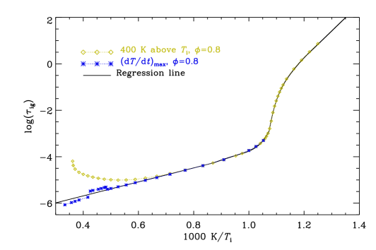
Figure 2: Ignition delay time as a function of temperature for two different definitions of the ignition delay time. The yellow line present the results found by defining ignition as the point where the temperature has reached 400 degrees above the initial temperature, while for the blue line ignition is defines as the time when the temperature gradient is at its maximum. The black line is a best fit to the blue line.

Fig. 2 shows how the ignition delay time depends on temperature. In the figure there are two data sets, where both are obtained from zero dimensional simulations with the Pencil Code. The two are based on different methods of ignition determination. It can be seen that they differ when the temperature is sufficiently high. This is due to the fact that for high temperatures an increasing amount of the chemical energy is converted into radicals instead of thermal energy. This means that above a certain preheat temperature the mixture temperature will not increase with as much as 400 K, and this leads to the very rapid increase of $\tau_{\mathrm{ig}}$ for definition 1).

The model use $\tau_{\mathrm{ig}}(T)$ together with the heat equation to predict if a mixture ignites or not, based on mixture composition and the initial parameters $T_{\mathrm{max}}$ and $r_{\mathrm{s_{0}}}$. Lets define an ignition progress variable $P$ such that $P=0$ at $t=0$ and $P=1$ when the system has reached ignition. If $P$ does not reach 1 this means that the mixture did not ignite, i.e. not enough energy was supplied to the system. An equation, which fulfill these requirements, is

$$P=\int\limits_{t=0}^{\infty}\!\frac{1}{\tau_{\mathrm{ig}}(T_{\mathrm{m}}(t))}\,\mathrm{d}t.$$ (17)

The rationale behind this equation is that in order for ignition to occur a certain amount of radicals are required. These radicals are produced at all temperatures above a certain limit. The rate of radical production is inversionally proportional to the ignition delay time.

Initially the parameters $T_{\mathrm{max}}$ and $r_{\mathrm{s_{0}}}$ are given. For each time step of lenght $\Delta t$, some heat diffuses away, and a new temperature, $T_{\mathrm{m}}(t+\Delta t)$, is obtained from Eq. (15). Based on the new temperature a new ignition delay time, $\tau_{\mathrm{ig}}\left(T_{\mathrm{m}}\left(t+\Delta t\right)\right)$, is obtained, which gives a new contribution to the ignition progress variable $P$. If, at any given time, P equals unity the current parameters and conditions have produced an ignition. As seen from Fig. 2, the lower the temperature gets, the higher the ignition delay time gets. This means that the term $1/\tau_{\mathrm{ig}}(T_{\mathrm{m}}(t))$ in Eq. (17) gets smaller, and each contribution towards $P$ for each time step gets smaller. If heat is diffused away too quickly $P$ will never reach 1, and the process will count as a non ignition case.

4 Results

In all of the following an hydrogen-air mixture with an equivalence ratio of 0.8 is considered.

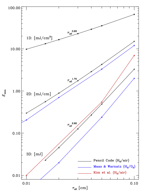
Figure 3: MIE as a function of ignition source radius for different dimensionality’s. Black line correspond to the DNS results from this work, blue line are the results for Maas & Warnatz (1998) [4] with a stoichiometric Hydrogen-Oxygen mixture while the red line is the results of Kim et al. (2004) [3] with a stoichiometric Hydrogen-Air mixture.

The ignition energy supplied to the mixture is

$$Q=\int_{V}c_{P}\rho(T-T_{0})dV^{\prime}$$ (18)

where $V$ is a large volume containing the ignition source and $T$ is given by Eq. (5). In order to find MIE for a given $r_{s}$ a series of simulations with gradually increasing $T_{\rm max}$ are run. By definition MIE equals $Q$ for the lowest temperature $T_{\rm max}$ at which the mixture is ignited. In Fig. 3 the MIE is shown as a function of ignition source radius for 1, 2 and 3 dimensional setups. For the three dimensional case our DNS results with the Pencil Code (black line) is slightly above the results of Maas & Warnatz (1998) [4], this is however as expected since Maas & Warnatz (1998) [4] considered pure Oxygen as oxidizer, while in the current work air has been used. Furthermore, it is seen that the DNS results are very similar to the results of Kim et al. (2004) [3], which was performed with a stoichiometric Hydrogen-Air mixture, except for the largest radius where the results of Kim et al. (2004) [3] bends upward. It is not known what cause the discrepancy for the largest radii.

For the two dimensional results it is once again seen that the Pencil-Code results correspond very well with the results of Maas & Warnatz (1998) [4] except for the vertical shift due to the differences in oxidizer.

For the one dimensional line there are no literature results with which it could be compared, but the trends nevertheless seems to be correct.

Naively one could think that the MIE would scale as $r_{s0}^{N}$ where $N$ is the dimensionality. Due to the stronger temperature gradients for smaller radii there will however be more thermal diffusion away from the center of the profile for smaller radii, and the MIE should therefore scale as $r_{s0}^{M}$ where $M<N$. This is indeed also what is found in the simulations where $M$ is 0.83, 1.70 and 2.62, for 1D, 2D and 3D, respectively.

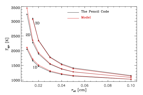
Figure 4: In this figure the results from the Pencil Code and the results from the simplified model are compared for all the dimensions.The parameters are $T_{0}=300$ K, $\phi=0.8$ and $P=1$ atm.

Lets define an ignition temperature $T_{\rm ign}(r_{s0})$, which is a function of the initial width of the distribution $r_{s0}$, such that for $T_{\rm max}<T_{\rm ign}(r_{s0})$ there is no ignition while for $T_{\rm max}>T_{\rm ign}(r_{s0})$ the mixture ignites. In Fig. 4 $T_{\rm ign}$ from the DNS simulations is shown as a function of $r_{s0}$ for the three different dimensionality’s (black line). It is clearly seen that as the width of the initial profile is decreased the required temperature for ignition increases strongly. This is because the temperature diffusion rate scale as the second order gradient, which for a Gaussian distribution means that $\partial T/\partial t\sim r_{s}(t)^{-2}$ (see Eq. (11)). Furthermore it is seen that the higher the dimensionality the higher is the required initial temperature. This comes from the fact that high dimensionality yields more degrees of freedom for the thermal diffusion, and consequently the temperature in the middle of the distribution decreases faster. This is seen in Eq. (15) where $\partial T/\partial t\propto N$.

The red lines in Fig. 4 show the results obtained with the new model. It is seen that the model results are very similar to the results from the full DNS. Thus it is clear that for the setup used here the new model is a very good alternative to the full DNS, and there are no obvious reasons why this should not be the case also for other fuels, equivalence ratios, ambient temperatures etc.

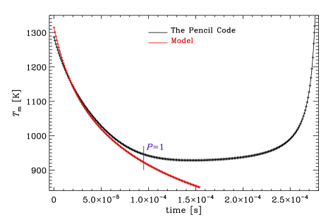
Figure 5: Temperature evolution for DNS (black line) and model (red line) results. The time where the ignition progress variable $P$ is unity is marked by the blue line. This example is taken from the one dimensional result with $r_{s0}=0.03$ cm.

In Fig. 5 the central temperature evolution is compared for the DNS results and the model results for the same specific case. The evolution is very similar for early times, but they are seen to deviate after $\sim 10^{-4}$ s when the mixture starts to burn (as we see in the results of DNS) and thus produce heat. This is however not a problem since the model calculations will be finalized when $P\geq 1$, meaning that ignition has been achieved, which for this particular case happened after $9.5\times 10^{-5}$ s. If, however, the initial temperature is lower, such that there will be no ignition, the model calculation will be stopped, with the conclusion that no ignition could be achieved, when $P$ has converged at a level below unity.

5 Conclusion

A new novel model for determining ignition has been described for the case of an initial Gaussian temperature distribution. The model, which require a functional description of the ignition delay time as input, is compared against fully resolved DNS results and found to produce very similar results. This indicate that what determines if an initial ignition kernel will evolve into a successful ignition or not relies on two tings; 1) the amount of thermal diffusion away from the center of the distribution and 2) the integrated value of the inverse ignition delay. It is also expected that diffusion of radicals out of the center of the distribution will have an effect on ignition, but this is apparently only of equal or less importance compared to the thermal diffusion.

Regarding the importance of the dimensionality of the heat source it is found that for higher dimensionality’s there are more degrees of freedom for the thermal diffusion, and consequently the temperature will decrease more quickly in such a distribution such that the required maximum temperature for ignition is higher for the higher dimensions.

References

- [1] Kurdyumov, V., Blasco, J., Sanchez, A. L. and Linan, A. Combustion and flame, 136, 394-397 (2004)
- [2] Kondo, S., Takahashi, A. and Tokuhashi, K. Journal of Hazardous Materials, A103, 11-23 (2003)
- [3] Kim, H. J., Chung, S. H. and Sohn, C. H. KSME International Journal, 18, 838-846 (2004)
- [4] U. Maas and J. Warnatz, COMBUSTION AND FLAME 74: 53-69 (1988)
- [5] R. Ono, M. Nifuko, S. Fujiwara, S. Horiguchi and T. Oda, Journal of Electrostatics 65 (2007) 87-93
- [6] The Pencil Code is a high-order finite-difference code (sixth order in space and third order in time); http://pencil-code.googlecode.com.
- [7] Babkovskaia, N., Haugen, N. E. L. and Brandenburg, A. Journal of Computational Physics, 230, 1-12 (2011)