Abstract. Estimating the number of spikes in a spiked model is an important problem in many areas such as signal processing. Most of the classical approaches assume a large sample size $n$ whereas the dimension $p$ of the observations is kept small. In this paper, we consider the case of high dimension, where $p$ is large compared to $n$. The approach is based on recent results of random matrix theory. We extend our previous results to a more difficult situation where some spikes are equal, and compare our algorithm to an existing benchmark method.

Keywords. Spiked population model, high-dimensional covariance matrix, random matrix theory, Tracy-Widom law.

1. Introduction

The spiked population model has been introduced in [Joh01], and appears in many scientific fields. In wireless communications, a signal emitted by a source is modulated and received by an array of antennas, and the reconstruction of the original signal is directly linked to the inference of “spikes”. In psychology literature, the strict factor model is equivalent to the spiked population model, and the number of factors has a primary importance [And03]. Similar models can be found in physics of mixture [KN08], [Nad] or population genetics. More precisely, we consider the following spiked population model for the observed signals $\mathsf{x}(t)$:

$$\mathsf{x}(t) = \sum_{k=1}^{q_{0}}f_{k}(t)a_{k}+\sigma n(t)=\mathsf{A}f(t)+\sigma n(t)\text{,}$$ (1)

where $f(t)=(f_{1}(t),\ldots,f_{q_{0}}(t))^{*}\in\mathbb{R}^{q_{0}}$ are $q_{0}$ independent random signals ($q_{0}<p$) with mean zero and unit variance; $\mathsf{A}=(a_{1},\ldots,a_{q_{0}})$ is a $p\times q_{0}$ full rank matrix (mixing weights); and $\sigma\in\mathbb{R}$ is the unknown noise level, $n(t)\sim\mathcal{N}(0,\mathsf{I}_{p})$ is a $p$-dimensional Gaussian white noise independent of $f(t)$.

The population covariance matrix $\Sigma$ of $\mathsf{x}(t)$ equals $\mathsf{A}\mathsf{A}^{*}+\sigma^{2}\mathsf{I}_{p}$ and has the spectral decomposition

$$\mathsf{W}^{*}\Sigma\mathsf{W}=\sigma^{2}\mathsf{I}_{p}+\mbox{diag}(\alpha_{1},\dots,\alpha_{q_{0}},0,\dots,0)$$

where $\mathsf{W}$ is an unknown basis of $\mathbb{R}^{p}$ and $\alpha_{1}\geq\alpha_{2}\geq\dots\geq\alpha_{q_{0}}>0$. As in [PY12], we rewrite the spectral decomposition of $\Sigma$ as

$$\mathsf{W}^{*}\Sigma\mathsf{W}=\sigma^{2}\mbox{diag}(\alpha_{1}^{\prime},\dots,\alpha_{q_{0}}^{\prime},1,\dots,1)\text{,}$$

with $\alpha_{i}^{\prime}=\alpha_{i}/\sigma^{2}+1$.

Notice that Model (1) is called a strict factor model in [And03]. It should not be confused with those factor model widely used in econometric and finance which have generally a more complex structure. For instance, the term strict factor model is used in these fields to refer to a noise with a general diagonal covariance, while in the so-called approximate factor model or the dynamic factor model (see e.g. [CR83] and [FHLR00]), the noise is cross-sectionally correlated unlike the white noise structure assumed in (1), and the factors $f(t)$ could be a time-series unlike the i.i.d. structure assumed in (1). In sum, these factor models have a much more complex structure than the spiked population model (1) considered in this paper.

A fundamental inference problem in Model (1) is the determination of the number of spikes $q_{0}$. Many methods have been developed, mostly based on information theoretic criteria, such as the minimum description length (MDL) estimator, Bayesian model selection or Bayesian Information Criteria (BIC) estimators, see [WK85] for a review. Nevertheless, these methods are based on asymptotic expansions for large sample size and may not perform well when the dimension of the data $p$ is large compared to the sample size $n$. To our knowledge, this problem in the context of high-dimension appears for the first time in [CS92]. Recent advances have been made using the random matrix theory by [Har] or Onatski [Ona09] in economics, and Kritchman & Nadler [KN08] in chemometric literature.

Several studies have also appeared in the area of signal processing from high-dimensional data. Everson & Roberts [ER00] proposed a method using both random matrix theory (RMT) and Bayesian inference, while Ulfarsson & Solo combined RMT and Stein’s unbiased risk estimator (SURE) in [US08]. In [NE08] and [Nad10], the authors proposed some estimators using information theoretic criteria. Finally in [KN09], Kritchman & Nadler constructed an estimator based on the distribution of the largest eigenvalue (hereafter refereed as the KN estimator). In [PY12], we have also introduced a new method based on recent results of [BY08] and [Pau07] in random matrix theory. It is worth mentioning that for high-dimensional time series, an empirical method for the estimation of the spike number has been recently proposed in [LYB11] and [LY12].

In all the cited references above, spikes are assumed to be distinct. However, we observe that when some of these spikes are close each other, the estimation problem becomes more difficult and these algorithms need to be modified. We refer this new situation as the case with possibly equal spikes and its precise formulation will be given in Section 2.2. The aim of this work is to extend our method [PY12] to this new situation and to compare it with the KN estimator, that is known in the literature as one of the best estimation methods.

The rest of the paper is organized as follows. In Section 2, the estimation problem of the number of possibly equal spikes is introduced, and our estimator is then proposed with a proof for its asymptotic consistency. Section 3 provides simulation experiments to assess the finite-sample quality of our estimator. In Section 4, we analyze the influence of a tuning parameter $C$ used in our procedure and propose an automatic calibration method of the parameter. Next, we carry out simulation experiments in Section 5 to compare our method to the benchmark KN estimator. Conclusions then follow and the appendix collects all the proofs.

2. Main results

The sample covariance matrix of the $n$ $p$-dimensional i.i.d. vectors considered at each time $t$, $(\mathsf{x}_{i}=\mathsf{x}(t_{i}))_{1\leq i\leq n}$ is

$$\mathsf{S}_{n}=\frac{1}{n}\sum_{i=1}^{n}\mathsf{x}_{i}\mathsf{x}_{i}^{*}\text{.}$$

Denote by $\lambda_{n,1}\geq\lambda_{n,2}\geq\dots\geq\lambda_{n,p}$ its eigenvalues. Our aim is to estimate $q_{0}$ on the basis of $\mathsf{S}_{n}$. We first recall our previous result of [PY12] in the case of different spikes. Next, we propose an extension of the algorithm to the case with possibly equal spikes. The consistency of the extended algorithm is established.

2.1. Previous work: estimation with different spikes

We consider the case where the $(\alpha_{i})_{1\leq i\leq q_{0}}$ are all different, so there are $q_{0}$ distinct spikes. It is assumed in the sequel that $p$ and $n$ are related so that when $n\rightarrow+\infty$, $p/n\rightarrow c>0$. Therefore, $p$ can be large compared to the sample size $n$ (high-dimensional case).

Moreover, we assumed that $\alpha_{1}^{\prime}>\dots>\alpha_{q_{0}}^{\prime}>1+\sqrt{c}$ for all $i\in\{1,\dots,q_{0}\}$; i.e all the spikes $\alpha_{i}$’s are greater than $\sigma^{2}\sqrt{c}$. For $\alpha\neq 1$, we define the function

$$\phi(\alpha)=\alpha+\frac{c\alpha}{\alpha-1}\text{.}$$

Baik and Silverstein [BS06] proved that, under a moment condition on $\mathsf{x}$, for each $k\in\{1,\dots,q_{0}\}$ and almost surely,

$$\lambda_{n,k}\longrightarrow\sigma^{2}\phi(\alpha_{k}^{\prime})\text{.}$$

They also proved that for all $1\leq i\leq L$ with a prefixed range $L$ and almost surely,

$$\lambda_{n,q_{0}+i}\rightarrow b=\sigma^{2}(1+\sqrt{c})^{2}\text{.}$$

The estimation method of $q_{0}$ in [PY12] is based on a close inspection of differences between consecutive eigenvalues

$$\delta_{n,j}=\lambda_{n,j}-\lambda_{n,j+1}\text{, }j\geq 1\text{.}$$

Indeed, the results quoted above imply that a.s. $\delta_{n,j}\rightarrow 0$, for $j\geq q_{0}$ whereas for $j<q_{0}$, $\delta_{n,j}$ tends to a positive limit. Thus it becomes possible to estimate $q_{0}$ from index-numbers $j$ where $\delta_{n,j}$ become small. More precisely, the estimator is

$$\hat{q}_{n} = \mbox{min}\{j\in\{1,\dots,s\}:\delta_{n,j+1}<d_{n}\}\text{,}$$ (2)

where $s>q_{0}$ is a fixed number big enough, and $d_{n}$ is a threshold to be defined. In practice, the integer $s$ should be thought as a preliminary bound on the number of possible spikes. In [PY12], we proved the consistency of $\hat{q}_{n}$ providing that the threshold satisfies $d_{n}\rightarrow 0$, $n^{2/3}d_{n}\rightarrow+\infty$ and under the following assumption on the entries of $\mathsf{x}$.

Assumption 1.

The entries $\mathsf{\mathsf{x}}^{i}$ of the random vector $\mathsf{\mathsf{x}}$ have a symmetric law and a sub-exponential decay, that means there exists positive constants $D$, $D^{\prime}$ such that, for all $t\geq D^{\prime}$,

$$\mathbb{P}(|\mathsf{\mathsf{x}}^{i}|\geq t^{D})\leq e^{-t}\text{.}$$

2.2. Estimation with possibly equal spikes

As said in the Introduction, when some spikes are close each other, estimation algorithms need to be modified. More precisely, we adopt the following theoretic model with $K$ different spike strengths $\alpha_{1},\dots,\alpha_{K}$, each of them can appear $n_{k}$ times (equal spikes), respectively. In other words,

$$\mbox{spec}(\Sigma) = (\underbrace{\alpha_{1},\dots,\alpha_{1}}_{n_{1}},\dots,\underbrace{\alpha_{K},\dots,\alpha_{K}}_{n_{K}},\underbrace{0,\dots,0}_{p-q_{0}})+\sigma^{2}(\underbrace{1,\dots,1}_{p})$$

$$= \sigma^{2}(\underbrace{\alpha_{1}^{\prime},\dots,\alpha_{1}^{\prime}}_{n_{1}},\dots,\underbrace{\alpha_{K}^{\prime},\dots,\alpha_{K}^{\prime}}_{n_{K}},\underbrace{1,\cdots,1}_{p-q_{0}})\text{.}$$

with $n_{1}+\dots+n_{K}=q_{0}$. When all the spikes are unequal, differences between sample spike eigenvalues tend to a positive constant, whereas with two equal spikes, such difference will tend to zero. This fact creates an ambiguity with those differences corresponding to the noise eigenvalues which also tend to zero. However, the convergence of the $\delta_{n,i}$’s, for $i>q_{0}$ (noise) is faster (in $O_{\mathbb{P}}(n^{-2/3})$) than that of the $\delta_{n,i}$ from equal spikes (in $O_{\mathbb{P}}(n^{-1/2})$) as a consequence of Theorem 3.1 of Bai & Yao [BY08]. This is the key feature we use to adapt the estimator (2) to the current situation with a new threshold $d_{n}$. The precise asymptotic consistency is as follows.

Theorem 1.

Let $(\mathsf{x}_{i})_{(1\leq i\leq n)}$ be $n$ copies i.i.d. of $\mathsf{x}$ which follows the model (1) and satisfies Assumption 1. Suppose that the population covariance matrix $\Sigma$ has $K$ non null and non unit eigenvalues $\alpha_{1}>\dots>\alpha_{K}>\sigma^{2}\sqrt{c}$ with respective multiplicity $(n_{k})_{1\leq k\leq K}$ ($n_{1}+\dots+n_{K}=q_{0}$), and $p-q_{0}$ unit eigenvalues. Assume that $\frac{p}{n}\rightarrow c>0$ when $n\rightarrow+\infty$. Let $(d_{n})_{n\geq 0}$ be a real sequence such that $d_{n}=o(n^{-1/2})$ and $n^{2/3}d_{n}\rightarrow+\infty$. Then the estimator $\hat{q}_{n}$ is consistent; i.e $\widehat{q}_{n}\rightarrow q_{0}$ in probability when $n\rightarrow+\infty$.

Compared to the previous situation, the only modification of our estimator is a new condition $d_{n}=o(n^{-1/2})$ on the convergence rate of $d_{n}$. The proof of Theorem 1 is postponed to Appendix.

There is a variation of the estimator defined as follows. Instead of making a decision once one difference $\delta_{k}$ is below the threshold $d_{n}$ (see (2)), one may decide once two consecutive differences $\delta_{k}$ and $\delta_{k+1}$ are both below $d_{n}$, i.e. define the estimator to be

$$\hat{q}_{n}^{*} = \mbox{min}\{j\in\{1,\dots,s\}:\delta_{n,j+1}<d_{n}\text{ and }\delta_{n,j+2}<d_{n}\}\text{.}$$ (3)

It can be easily checked that the proof for the consistency of $\hat{q}_{n}$ applies equally to $\hat{q}_{n}^{*}$ under the same conditions as in Theorem 1. This version of the estimator will be used in all the simulation experiments below. Intuitively, $\hat{q}_{n}^{*}$ should be more robust than $\hat{q}_{n}$. We notice that eventually more than two consecutive differences could be used in (3). However, our simulation experiments have shown that using more consecutive differences does not improve significantly. So we limit ourselves the simulation study to two consecutive differences.

3. Implementation issues and overview of simulation experiments

The practical implementation of the estimator $\hat{q}_{n}^{*}$ depend on two unknown parameters, namely the noise variance $\sigma^{2}$ and the threshold sequence $d_{n}$. As for an estimate of $\sigma^{2}$, we used in [PY12] an algorithm based on the maximum likelihood estimate

$$\widehat{\sigma}^{2}=\frac{1}{p-q_{0}}\sum_{i=q_{0}+1}^{p}\lambda_{n,i}\text{.}$$

As explained in [KN08] and [KN09], this estimator has a negative bias. Hence the authors developed an improved estimator with a smaller bias. We will use this improved estimator of the noise level when it is unknown.

It remains to choose a threshold sequence $d_{n}$. As argued in [PY12], we use a sequence $d_{n}$ of the form $Cn^{-2/3}\sqrt{2\log\log n}$, where $C$ is a “tuning” parameter to be adjusted. In our Monte-Carlo experiments, we shall consider two choices of $C$: the first one is manually tuned and used to assess some theoretical properties of the estimator $\hat{q}_{n}^{*}$; and the second one is a data-driven and automatically chosen value that is used in real-life applications. This automatic choice is introduced in Section 4.

In the remaining of the paper, we conduct extensive simulation experiments to assess the quality of the estimator $\hat{q}_{n}^{*}$ including a detailed comparison with a benchmark detector from the literature.

In all experiments, data are generated with the assigned noise level $\sigma^{2}=1$ and empirical values are calculated using 500 independent replications. Table 1 gives a summary of the parameters in the experiments. One should notice that both the given value of $\sigma^{2}=1$ and the estimated one, as well as the manually tuned and the automatic chosen values of $C$ are used in different scenarios. There are in total three sets of experiments. The first set (Figures 1-2 and Models A, B), given in this section, illustrates the convergence of our estimator in the situation of equal spikes. The second set of experiments (Figures 3-4 and Models D-K) addresses the performance of the automatic tuned $C$ and they are reported in Section 4. The last set of experiments (Figures 5-6-7), reported in Section 5, are designed for a comparison with the benchmark detector KN.

Table 1. Summary of parameters used in the simulation experiments. (L: left, R: right)

Fig.	Mod.	spike	Fixed parameters				Var.
No.	No.	values	$p,n$	$c$	$\sigma^{2}$	$C$	par.
1		($\alpha$)	$(200,800)$	1/4	Given	$5.5$	$\alpha$
			$(2000,500)$	4		9
2	A	$(\alpha,\alpha,5)$	$(200,800)$	$1/4$	Given	$6$	$\alpha$
	B	$(\alpha,\alpha,15)$	$(2000,500)$	$4$		$9.9$
3L	D	$(6,5)$		10	Given	11 and auto	$n$
	E	$(6,5,5)$
3R	F	$(10,5)$		1	Given	5 and auto	$n$
	G	$(10,5,5)$
4L	H	$(1.5)$		1	Given	5 and auto	$n$
	I	$(1.5,1.5)$
4R	J	$(2.5,1.5)$		1	Given	5 and auto	$n$
	K	$(2.5,1.5,1.5)$
5L	D	$(6,5)$		10	Estimated	Auto	$n$
5R	J	$(2.5,1.5)$		1	Estimated	Auto	$n$
6L	E	$(6,5,5)$		10	Estimated	Auto	$n$
6R	K	$(2.5,1.5,1.5)$		1	Estimated	Auto	$n$
7	L	No spike		$1$	Estimated	Auto	$n$
				$10$

3.1. Comparison between the case of equal spikes and different spikes

In Figure 1, we consider the case of a single spike $\alpha$ and analyze the probability of misestimation as a function of the value of $\alpha$, for $(p,n)=(200,800)$, $c=0.25$ and $(p,n)=(2000,500)$, $c=4$. We set $C=5.5$ for the first case and $C=9$ for the second case (all manually tuned). The noise level $\sigma^{2}=1$ is given. The estimator performs well: we recover the threshold from which the behavior of the spike eigenvalues differ from the noise ones ($\sqrt{c}=0.5$ for the first case, and $2$ for the second).

Figure 1. Misestimation rates as a function of spike strength for $(p,n)=(200,800)$ and $(p,n)=(2000,500)$.

Next we keep the same parameters while adding some equal spikes. In Figure 2, we consider Model A: $(\alpha_{1},\alpha_{2},\alpha_{3})=(\alpha,\alpha,5)$, $0\leq\alpha\leq 2.5$ and Model B: $(\alpha_{1},\alpha_{2},\alpha_{3})=(\alpha,\alpha,15)$, $0\leq\alpha\leq 8$. The dimensions are $(p,n)=(200,800)$ and $C=6$ for Model A, and $(p,n)=(2000,500)$ and $C=9.9$ for Model B.

Figure 2. Misestimation rates as a function of spike strength for $(p,n)=(200,800)$, Model A and $(p,n)=(2000,500)$, Model B.

There is no particular difference with the previous situation: when spikes are close or even equal, or near to the critical value, the estimator remains consistent although the convergence rate becomes slower. Overall, these experiments demonstrate that the proposed estimator is able to find the number of spikes.

4. On the choice of $C$: an automatic calibration procedure

In the previous experiments, the tuning parameter $C$ has been selected manually on a case by case basis. This is however untenable in a real-life situation. We now provide an automatic calibration of this parameter. The idea is to use the difference of the two largest eigenvalues of a Wishart matrix (which correspond to the case of no spike): indeed, our algorithm should stop once two consecutive eigenvalues are below the threshold $d_{n}$ corresponding to a noise eigenvalue. As we do not know precisely the distribution of the difference between eigenvalues of a Wishart matrix, we approximate the distribution of the difference between the two largest eigenvalues $\tilde{\lambda}_{1}-\tilde{\lambda}_{2}$ by simulation under 500 independent replications. We then take the mean $s$ of the 10th and the 11th largest spacings, so $s$ has the empirical probability $\mathbb{P}(\tilde{\lambda}_{1}-\tilde{\lambda}_{2}\leq s)=0.98$: this value will give reasonable results. We calculate a $\widetilde{C}$ by multiplying this threshold by $n^{2/3}/\sqrt{2\times\log\log(n)}$. The result for various $(p,n)$, with $c=1$ and $c=10$ are displayed in Table 2.

Table 2. Approximation of the threshold $s$ such that $\mathbb{P}(\tilde{\lambda}_{1}-\tilde{\lambda}_{2}\leq s)=0.98$.

(p,n)	(200,200)	(400,400)	(600,600)	(2000,200)	(4000,400)	(7000,700)
Value of $s$	0.340	0.223	0.170	0.593	0.415	0.306
$\widetilde{C}$	6.367	6.398	6.277	11.106	11.906	12.44

The values of $\widetilde{C}$ are quite close to the values we would have chosen in similar settings (For instance, $C=5$ for $c=1$ and $C=9.9$ or 11 for $c=10$), although they are slightly higher. Therefore, this automatic calibration of $\widetilde{C}$ can be used in practice for any data and sample dimensions $p$ and $n$.

To assess the quality of the automatic calibration procedure, we run some simulation experiments using both $\widetilde{C}$ and the manually tuned $C$. We consider in Figure 3 the case $c=10$. On the left panel we consider Model D ($\alpha=(6,5)$) and Model E ($\alpha=(6,5,5)$) (upper curve). On the right panel we have Model F ($\alpha=(10,5)$) and Model G ($\alpha=(10,5,5)$) (upper curve). The dotted lines are the results with $C$ manually tuned.

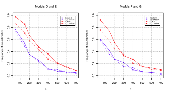
Figure 3. Misestimation rates as a function of $n$ for Models D, E (left) and Models F, G (right).

Using the automatic value $\tilde{C}$ causes only a slight deterioration of the estimation performance. We observe significantly higher error rates in the case of equal spikes for moderate sample sizes.

The case $c=1$ is considered in Figure 4 with Models H ($\alpha=1.5$) and I ($\alpha=(1.5,1.5)$) (upper curve) on the left and Model J ($\alpha=(2.5,1.5)$) and K ($\alpha=(2.5,1.5,1.5)$) (upper curve) on the right.

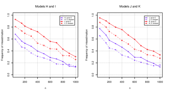
Figure 4. Misestimation rates as a function of $n$ for Models H, I (left) and Models J, K (right).

Compared to the previous situation of $c=10$, using the automatic value $\widetilde{C}$ affects a bit more our estimator (up to 20% of degradation). Nevertheless, the estimator remains consistent. Furthermore, we have to keep in mind that our simulation experiments have considered critical cases where spikes eigenvalues are close: in many of practical applications, theses spikes are more separated so that the influence of $C$ will be less important.

5. Method of Kritchman & Nadler and comparison

5.1. Algorithm of Kritchman & Nadler

In their papers [KN08] and [KN09], Kritchman & Nadler develop a different method to estimate the number of spikes. In this section we compare by simulation our estimator (PY) with this method (KN). Notice that these authors have compared their estimator KN with existing estimators in the signal processing literature, based on the minimum description length (MDL), Bayesian information criterion (BIC) and Akaike information criterion (AIC) [WK85]. In most of the studied cases, the estimator KN performs better. Furthermore in [Nad10], this estimator is compared to an improved AIC estimator and it still has a better performance. Thus we decide to consider only this estimator KN for the comparison here.

In the absence of spikes, $n\mathsf{S}_{n}$ follows a Wishart distribution with parameters $n,p$. In this case, Johnstone [Joh01] has provided the asymptotic distribution of the largest eigenvalue of $\mathsf{S}_{n}$.

Proposition 1.

Let $\mathsf{S}_{n}$ be the sample covariance matrix of $n$ vectors distributed as $\mathcal{N}(0,\sigma^{2}\mathsf{I}_{p})$, and $\lambda_{n,1}\geq\lambda_{n,2}\geq\dots\geq\lambda_{n,p}$ be its eigenvalues. Then, when $n\rightarrow+\infty$, such that $\frac{p}{n}\rightarrow c>0$

$$\mathbb{P}\left(\frac{\lambda_{n,1}}{\sigma^{2}}<\frac{\beta_{n,p}}{n^{2/3}}s+b\right)\rightarrow F_{1}(s)\mbox{, }s>0$$

where $b=(1+\sqrt{c})^{2}$, $\beta_{n,p}=\left(1+\sqrt{\frac{p}{n}}\right)\left(1+\sqrt{\frac{n}{p}}\right)^{\frac{1}{3}}$ and $F_{1}$ is the Tracy-Widom distribution of order 1.

Assume the variance $\sigma^{2}$ is known. To distinguish a spike eigenvalue $\lambda$ from a noise one at an asymptotic significance level $\gamma$, their idea is to check whether

$$\lambda_{n,k}>\sigma^{2}\left(\frac{\beta_{n,p-k}}{n^{2/3}}s(\gamma)+b\right)$$ (4)

where $s(\gamma)$ verifies $F_{1}(s(\gamma))=1-\gamma$ and can be found by inverting the Tracy-Widom distribution. This distribution has no explicit expression, but can be computed from a solution of a second order Painlevé ordinary differential equation. The estimator KN is based on a sequence of nested hypothesis tests of the following form: for $k=1,2,\ldots,\mbox{min}(p,n)-1$,

$$\mathcal{H}_{0}^{(k)}\mbox{: }q_{0}\leq k-1\quad vs.\quad\mathcal{H}_{1}^{(k)}\mbox{: }q_{0}\geq k\mbox{ .}$$

For each value of $k$, if (4) is satisfied, $\mathcal{H}_{0}^{(k)}$ is rejected and $k$ is increased by one. The procedure stops once an instance of $\mathcal{H}_{0}^{(k)}$ is accepted and the number of spikes is then estimated to be $\tilde{q}_{n}=k-1$. Formally, their estimator is defined by

$$\tilde{q}_{n}=\underset{k}{\mbox{argmin}}\left(\lambda_{n,k}<\widehat{\sigma}^{2}\left(\frac{\beta_{n,p-k}}{n^{2/3}}s(\gamma)+b\right)\right)-1\text{.}$$

Here $\widehat{\sigma}$ is some estimator of the noise level (as discussed in Section 3). The authors proved the strong consistency of their estimator as $n\rightarrow+\infty$ with fixed $p$, by replacing the fixed confidence level $\gamma$ with a sample-size dependent one $\gamma_{n}$, where $\gamma_{n}\rightarrow 0$ sufficiently slow as $n\rightarrow+\infty$. They also proved that $\lim_{p,n\rightarrow+\infty}\mathbb{P}\left(\tilde{q}_{n}\geq q_{0}\right)=1$.

It is important to notice here that the construction of the KN estimator differs form ours, essentially because of the fixed alarm rate $\gamma$. We will discuss the issue of the false alarm rate in the last section.

5.2. Comparison with our method

In order to follow a real-life situation, we assume that $\sigma^{2}=1$ is unknown and we estimate it for both methods. Furthermore, we use the automatic calibration procedure to choose the constant $C$ in our method. We give a value of $\gamma=0.5\%$ to the false alarm rate of the estimator KN, as suggested in [KN09] and use their algorithm available at the author’s homepage.

We consider in Figure 5 Model D: $(\alpha_{1},\alpha_{2})=(6,5)$ and and Model J: $(\alpha_{1},\alpha_{2})=(2.5,1.5)$.

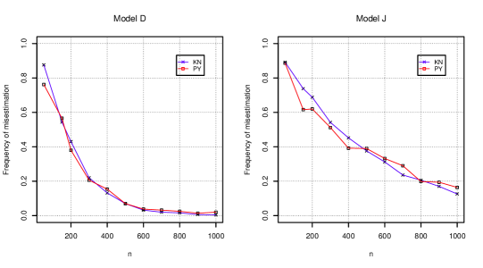
Figure 5. Misestimation rates as a function of $n$ for Model D (left) and Model J (right).

For both Model D and J, the performances of the two estimator are close. However the estimator PY is slightly better for moderate values of $n$ ($n\leq 400$) while the estimator KN has a slightly better performance for larger $n$. The difference between the two estimators are more important for Model J (up to 5% improvement).

Next we consider in Figure 6 Model E: $(\alpha_{1},\alpha_{2},\alpha_{2})=(6,5,5)$ and Model K: $(\alpha_{1},\alpha_{2},\alpha_{2})=(2.5,1.5,1.5)$, two models analogous to Model D and J but with two equal spikes.

Figure 6. Misestimation rates as a function of $n$ for Model E (left) and Model K (right).

For Model E, the estimator PY shows superior performance for $n\leq 500$ (up to 20% less error): adding an equal spike affects more the performance of the estimator KN. The difference between the two algorithms for Model K is higher than in the previous cases; the estimator PY performs better in all cases, up to 10%.

In Figure 7 we examine a special case with no spike at all (Model L). The estimation rates become the so-called false-alarm rate, a concept widely used in signal processing literature. The cases of $c=1$ and $c=10$ with $\sigma^{2}=1$ given are considered.

Figure 7. False-alarm rates as a function of $n$ for $c=1$ (left) and $c=10$ (right).

In both situations, the false-alarm rates of two estimators are quite low (less than 4%), and the KN one has a better performance.

In summary, in most of situations reported here, our algorithm compares favorably to an existing benchmark method (the KN estimator). It is also important to notice a fundamental difference between these two estimators: the KN estimator is designed to keep the false alarm rate at a very low level while our estimator attempts to minimize an overall misestimation rate. We develop more in details these issues in next section.

5.3. Influence of $C$ on the misestimation and false alarm rate

In the previous simulation experiments, we have chosen to report the misestimation rates. However, to have a fair comparison to either the KN estimator or any other method of the number of spikes, the different methods should have comparable false alarm probabilities. This section is devoted to an analysis of possible relationship between the constant $C$ and the implied false alarm rate. Following [KN09], the false alarm rate $\gamma$ of such an algorithm can be viewed as the type I error of the following test

$$\mathcal{H}_{0}\mbox{: }q_{0}=0\quad vs.\quad\mathcal{H}_{1}\mbox{: }q_{0}>0\mbox{,}$$

that is the probability of overestimation in the white noise case. Recall the step $k$ of the algorithm KN tests

$$\mathcal{H}_{0}^{(k)}\mbox{: }q_{0}\leq k-1\quad vs.\quad\mathcal{H}_{1}^{(k)}\mbox{: }q_{0}\geq k\mbox{.}$$

In [KN09], the authors argue that their threshold is determined such that

$$\mathbb{P}(\mbox{reject }\mathcal{H}_{0}^{(k)}|\mathcal{H}_{0}^{(k)})\approx\gamma\text{.}$$

More precisely, they give an asymptotic bound of the overestimation probability: they show that for $n=500$ and $p>10$, this probability is close to $\gamma$.

Since for our method, we do not know explicitly the corresponding false alarm rate, we recall in Table 3 the results from Figure 7, which were for the cases $c=1$ and $c=10$, with the automatic value $\tilde{C}$, under 500 independent replications.

Table 3. False alarm rates in case of $c=1$ and $c=10$.

(p,n)	(150,150)	(300,300)	(500,500)	(700,700)
PY	0.056	0.028	0.022	0.016
KN	0.008	0.002	0.001	0.000
(p,n)	(1500,150)	(3000,300)	(5000,500)	(7000,700)
PY	0.03	0.08	0.026	0.016
KN	0.004	0.006	0.004	0.006

As seen previously, the false alarm rates of our algorithm are much higher than the false alarm rate $\gamma=0.5\%$ of the KN estimator. Nevertheless, and contrary to the KN estimator, the overestimation rate of our estimator will be different from the false alarm rate, and will depend on the number of spikes and their values. Indeed, we use the gaps between two eigenvalues, instead of each eigenvalue separately. Consequently, there is no justification to claim that the probability $\mathbb{P}(\hat{q}_{n}>q|q=q_{0})$, for $q_{0}>1$ will be close to $\mathbb{P}(\hat{q}_{n}>0|q=0)$. To illustrate this phenomenon, we use the settings of Model E and K ($q_{0}=3$) and we evaluate the overestimation rate using 500 independent replications (note that the corresponding false alarm rates are those in Table 3). The results are displayed in Table 4.

Table 4. Empirical overestimation rates from Model E ($\alpha=(6,5,5)$, $c=10$) and Model K ($\alpha=(2.5,1.5,1.5)$, $c=1$).

	(p,n)	(1500,150)	(3000,300)	(5000,500)	(7000,700)
Model E	PY	0.004	0.022	0.018	0.01
	KN	0.000	0.000	0.000	0.000
	(p,n)	(150,150)	(300,300)	(500,500)	(700,700)
Model K	PY	0.006	0.002	0.002	0.006
	KN	0.000	0.000	0.000	0.000

We observe that these overestimation rates are lower than the false alarm rates given in Table 2: this suggests that no obvious relationship exists between the false alarm rate $\gamma$ and the overestimation rates for our algorithm.

Furthermore, the overestimation rates of the KN estimator are $0$ in all cases: it means that misestimation is mostly underestimated.

In summary, if the goal is to keep overestimation rates at a constant and low level, one should employ the KN estimator without hesitation (since by construction, the probability of overestimation is kept to a very low level). Otherwise, if the goal is also to minimize the overall misestimation rates i.e. including underestimation errors, our algorithm can be a good substitute to the KN estimator. One could think of choosing $C$ in each case to have a probability of overestimation kept fixed at a low level, but in this case the probability of underestimation would be high and the performance of the estimation would be poor: our estimator is constructed to minimize the overall misestimation rate.

6. Concluding remarks

In this paper we have considered the problem of the estimation of the number of spikes in high-dimensional data. When some spikes have close or even equal values, the estimation becomes harder and existing algorithm need to be re-examined or corrected. In this spirit, we have proposed a new version of our previous algorithm. Its asymptotic consistency is established. We compare our algorithm to an existing competitor proposed by Kritchman & Nadler (KN, [KN08], [KN09]). From our extensive simulation experiments in various scenarios, overall our estimator can have smaller misestimation rates, especially in cases with close and relatively low spike values (Figure 6) or more generally for almost all the cases provided that the sample size $n$ is moderately large ($n\leq 400$ or 500). Nevertheless, if the primary aim is to fix the false alarm rate and the overestimation rates at a very low level, the KN estimator is preferable.

Our algorithm depends on a tuning parameter $C$. By comparison, the KN estimator is remarkably robust and a single value of $\gamma=0.5\%$ was used in all the experiments. In Section 5 we have provided a first approach to an automatic calibration of $C$ which is quite satisfactory. More investigation is needed in the future for this calibration in order to further improve the performance of our estimator.

Acknowledgment The authors are grateful to two Referees and the Associate Editor for their helpful comments that have led to many improvements of the paper.

Appendix A Proof of Theorem 1

Without loss of generality we will assume that $\sigma^{2}=1$ (if it is not the case, we consider $\frac{\lambda_{n,j}}{\sigma^{2}}$). For the proof, we need the following Propositions 2 and 3 from the literature. Proposition 2 is a result of Bai and Yao [BY08] which derives from a CLT for the $n_{k}$-packed eigenvalues

$$\sqrt{n}[\lambda_{n,j}-\phi(\alpha_{k}^{\prime})]\mbox{, }j\in J_{k}$$

where $J_{k}=\{s_{k-1}+1,\dots,s_{k}\}$, $s_{i}=n_{1}+\cdots+n_{i}$ for $1\leq i\leq K$.

Proposition 2.

Assume that the entries $\mathsf{x}^{i}$ of $\mathsf{x}$ satisfy $\mathbb{E}(\|\mathsf{x}^{i}\|^{4})<+\infty$, $\alpha_{j}^{\prime}~{}>~{}1+\sqrt{c}$ for all $1\leq j\leq K$ and have multiplicity $n_{1},\dots,n_{K}$ respectively. Then as $p$, $n\rightarrow+\infty$ so that $\frac{p}{n}\rightarrow c$, the $n_{k}$-dimensional real vector

$$\sqrt{n}\{\lambda_{n,j}-\phi(\alpha_{k}^{\prime})\mbox{, }j\in J_{k}\}$$

converges weakly to the distribution of the $n_{k}$ eigenvalues of a Gaussian random matrix whose covariance depends on $\alpha_{k}^{\prime}$ and $c$.

Proposition 3 is a direct consequence of Proposition 5.8 from Benaych-Georges, Guionnet and Maida [BGGM11]:

Proposition 3.

Assume that the entries $\mathsf{x}^{i}$ of $\mathsf{x}$ have a symmetric law and a sub-exponential decay, that means there exists positive constants D, D’ such that, for all $t\geq\mbox{D'}$, we have $\mathbb{P}(|\mathsf{x}^{i}|~{}\geq~{}t^{D})~{}\leq~{}e^{-t}$. Then, for all $1\leq i\leq L$ with a prefixed range $L$,

$$n^{\frac{2}{3}}(\lambda_{n,q_{0}+i}-b)=O_{\mathbb{P}}(1)\text{.}$$

We also need the following lemma:

Lemma 1.

Let $(\mathsf{X}_{n})_{n\geq 0}$ be a sequence of positive random variables which weakly converges to a probability distribution with a continuous cumulative distribution function. Then for all real sequence $(u_{n})_{n\geq 0}$ which converges to 0,

$$\mathbb{P}(\mathsf{X}_{n}\leq u_{n})\rightarrow 0\text{.}$$

Proof.

As $(\mathsf{X}_{n})_{n\geq 0}$ converges weakly, there exists a function $G$ such that, for all $v\geq 0$, $\mathbb{P}(\mathsf{X}_{n}~{}\leq~{}v)\rightarrow G(v)$. Furthermore, as $u_{n}\rightarrow 0$, there exists $N\in\mathbb{N}$ such that for all $n~{}\geq~{}N$, $u_{n}~{}\leq~{}v$. So $\mathbb{P}(\mathsf{X}_{n}\leq u_{n})\leq\mathbb{P}(\mathsf{X}_{n}\leq v)$, and $\varlimsup\limits_{n\to+\infty}\mathbb{P}(\mathsf{X}_{n}\leq u_{n})\leq\varlimsup\limits_{n\to+\infty}\mathbb{P}(\mathsf{X}_{n}~{}\leq~{}v)=G(v)$. Now we can take $v\rightarrow 0$: as $(\mathsf{X}_{n})_{n\geq 0}$ is positive, $G(v)\rightarrow 0$. Consequently, $\mathbb{P}(\mathsf{X}_{n}~{}\leq~{}u_{n})\rightarrow~{}0\text{.}$ ∎

Proof.

of Theorem 1. The proof is essentially the same as Theorem 3.1 in [PY12], except when the spikes are equal. We have

$$\{\hat{q}_{n}=q_{0}\} =\{q_{0}=\mbox{min}\{j:\delta_{n,j+1}<d_{n}\}\}$$

$$=\{\forall j\in\{1,\dots,q_{0}\}\mbox{, }\delta_{n,j}\geq d_{n}\}\cap\{\delta_{n,q_{0}+1}<d_{n}\}\text{.}$$

Therefore

$$\mathbb{P}(\hat{q}_{n}=q_{0}) =\mathbb{P}\left(\bigcap_{1\leq j\leq q_{0}}\{\delta_{n,j}\geq d_{n}\}\cap\{\delta_{n,q_{0}+1}<d_{n}\}\right)$$

$$=1-\mathbb{P}\left(\bigcup_{1\leq j\leq q_{0}}\{\delta_{n,j}<d_{n}\}\cup\{\delta_{n,q_{0}+1}\geq d_{n}\}\right)$$

$$\geq 1-\sum_{j=1}^{q_{0}}\mathbb{P}(\delta_{n,j}<d_{n})-\mathbb{P}(\delta_{n,q_{0}+1}\geq d_{n})\text{.}$$

Case of $j=q_{0}+1$. In this case, $\delta_{n,q_{0}+1}=\lambda_{n,q_{0}+1}-\lambda_{n,q_{0}+2}$ (noise eigenvalues). As $d_{n}\rightarrow 0$ such that, $n^{2/3}d_{n}\rightarrow+\infty$, and by using Proposition 3 in the same manner as in the proof of Theorem 3.1 in [PY12], we have

$$\mathbb{P}(\delta_{n,q_{0}+1}\geq d_{n})\rightarrow 0\text{.}$$

Case of $1\leq j\leq q_{0}$. These indexes correspond to the spike eigenvalues.

• Let $I_{1}=\{1\leq l\leq q_{0}|\mbox{card}(J_{l})=1\}$ (simple spike) and $I_{2}=\{l-1|l\in I_{1}\text{ and }l-1>1\}$. For all $j\in I_{1}\cup I_{2}$, $\delta_{n,j}$ corresponds to a consecutive difference of $\lambda_{n,j}$ issued from two different spikes, so we can still use Proposition 3 and the proof of Theorem 3.1 in [PY12] to show that

  $$\mathbb{P}(\delta_{n,j}<d_{n})\rightarrow 0\mbox{, }\forall j\in I_{1}\text{.}$$

• Let $I_{3}=\{1\leq l\leq q_{0}-1|l\notin(I_{1}\cup I_{2})\}$. For all $j\in I_{3}$, it exists $k\in\{1,\dots,K\}$ such that $j\in J_{k}$.

  • If $j+1\in J_{k}$ then, by Proposition 2, $\mathsf{X}_{n}=\sqrt{n}\delta_{n,j}$ converges weakly to a limit which has a density function on $\mathbb{R}^{+}$. So by using Lemma 1 and that $d_{n}=o(n^{-1/2})$, we have

    $$\mathbb{P}\left(\delta_{n,j}<d_{n}\right)=\mathbb{P}\left(\sqrt{n}\delta_{n,j}<\sqrt{n}d_{n}\right)\rightarrow 0\text{;}$$

  • Otherwise, $j+1\notin J_{k}$, so $\alpha_{j}\neq\alpha_{j+1}$. Consequently, as previously, $\delta_{n,j}$ corresponds to a consecutive difference of $\lambda_{n,j}$ issued from two different spikes, so we can still use Proposition 2 and the proof of Theorem 3.1 in [PY12] to show that

    $$\mathbb{P}(\delta_{n,j}<d_{n})\rightarrow 0\text{.}$$

• The case of $j=q_{0}$ is considered as in [PY12].

Conclusion. $\mathbb{P}(\delta_{n,q_{0}+1}\geq d_{n})\rightarrow 0$ and $\sum_{j=1}^{q_{0}}\mathbb{P}(\delta_{n,j}<d_{n})\rightarrow 0$, therefore

$$\mathbb{P}(\hat{q}_{n}=q_{0})\underset{n\rightarrow+\infty}{\longrightarrow}1\text{.}$$

∎

References

- [And03] T. W. Anderson. An introduction to multivariate statistical analysis. Wiley Series in Probability and Statistics. Wiley-Interscience [John Wiley & Sons], Hoboken, NJ, third edition, 2003.
- [BGGM11] F. Benaych-Georges, A. Guionnet, and M. Maida. Fluctuations of the extreme eigenvalues of finite rank deformations of random matrices. Electron. J. Probab., 16(60):1621–1662, 2011.
- [BS06] Jinho Baik and Jack W. Silverstein. Eigenvalues of large sample covariance matrices of spiked population models. J. Multivariate Anal., 97(6):1382–1408, 2006.
- [BY08] Zhidong Bai and Jian-feng Yao. Central limit theorems for eigenvalues in a spiked population model. Ann. Inst. Henri Poincaré Probab. Stat., 44(3):447–474, 2008.
- [CR83] Florent Chamberlain, Gary and Michael Rothschild. Arbitrage, factor structure, and mean-variance analysis on large asset markets. Econometrica, 51(5):1281–1304, 1983.
- [CS92] L. Combettes and Jack W. Silverstein. Signal detection via spectral theory of large dimensional random matrices. IEEE Trans. Signal Process., 40(8):2100–2105, 1992.
- [ER00] Richard Everson and Stephen Roberts. Inferring the eigenvalues of covariance matrices from limited, noisy data. IEEE Trans. Signal Process., 48(7):2083–2091, 2000.
- [FHLR00] Mario Forni, Marc Hallin, Marco Lippi, and Lucrezia Reichlin. The generalized dynamic factor model: identification and estimation. Rev. Econom. Statist., 82(4):540–554, 2000.
- [Har] M.C. Harding. Estimating the number of factors in large dimensional factor models. Preprint.
- [Joh01] Iain M. Johnstone. On the distribution of the largest eigenvalue in principal components analysis. Ann. Statist., 29(2):295–327, 2001.
- [KN08] Shira Kritchman and Boaz Nadler. Determining the number of components in a factor model from limited noisy data. Chem. Int. Lab. Syst., 94, 2008.
- [KN09] Shira Kritchman and Boaz Nadler. Non-parametric detection of the number of signals: Hypothesis testing and random matrix theory. IEEE Trans. Signal Process., 57(10):3930–3941, 2009.
- [LY12] C. Lam and Q. Yao. Factor modeling for high-dimensional time series: inference for the number of factors. Ann. Statist., 40(2):694–726, 2012.
- [LYB11] C. Lam, Q. Yao, and N. Bathia. Estimation of latent factors for high-dimensional time series. Biometrika, 98:901–918, 2011.
- [Nad] Boaz Nadler. User-friendly guide to multivariate calibration and classification. NIR Publications, Chichester.
- [Nad10] Boaz Nadler. Nonparametric detection of signals by information theoretic criteria: performance analysis and an improved estimator. IEEE Trans. Signal Process., 58(5):2746–2756, 2010.
- [NE08] Raj Rao Nadakuditi and Alan Edelman. Sample eigenvalue based detection of high-dimensional signals in white noise using relatively few samples. IEEE Trans. Signal Process., 56(7, part 1):2625–2638, 2008.
- [Ona09] Alexei Onatski. Testing hypotheses about the numbers of factors in large factor models. Econometrica, 77(5):1447–1479, 2009.
- [Pau07] Debashis Paul. Asymptotics of sample eigenstructure for a large dimensional spiked covariance model. Statist. Sinica, 17(4):1617–1642, 2007.
- [PY12] Damien Passemier and Jian-feng Yao. On determining the number of spikes in a high-dimensional spiked population model. Random Matrices: Theory and Applications, 1(1):1150002, 2012.
- [US08] Magnus O. Ulfarsson and Victor Solo. Dimension estimation in noisy PCA with SURE and random matrix theory. IEEE Trans. Signal Process., 56(12):5804–5816, 2008.
- [WK85] Mati Wax and Thomas Kailath. Detection of signals by information theoretic criteria. IEEE Trans. Acoust. Speech Signal Process., 33(2):387–392, 1985.