Equivalence of Wilson Loops in ABJM and $\mathcal{N}=4$ SYM Theory

Abstract

In previous investigations, it was found that four-sided polygonal light-like Wilson loops in ABJM theory calculated to two-loop order have the same form as the corresponding Wilson loop in $\mathcal{N}=4$ SYM at one-loop order. Here we study light-like polygonal Wilson loops with $n$ cusps in planar three-dimensional Chern-Simons and ABJM theory to two loops. Remarkably, the result in ABJM theory precisely agrees with the corresponding Wilson loop in $\mathcal{N}=4$ SYM at one-loop order for arbitrary $n$. In particular, anomalous conformal Ward identites allow for a so-called remainder function of conformal cross ratios for $n\geq 6$, which is found to be trivial at two loops in ABJM theory in the same way as it is trivial in $\mathcal{N}=4$ SYM at one-loop order. Furthermore, the result for arbitrary $n$ obtained here, allows for a further investigation of a Wilson loop / amplitude duality in ABJM theory, for which non-trivial evidence was recently found by a calculation of four-point amplitudes that match the Wilson loop in ABJM theory.

I Introduction

Our motivation to consider polygonal light-like Wilson loops in 3d Chern-Simons and $\mathcal{N}=6$ superconformal Chern-Simons (ABJM) theory Aharony:2008ug stems from the Wilson loop/scattering amplitude duality in $\mathcal{N}=4$ super Yang-Mills.

In planar $\mathcal{N}=4$ super Yang-Mills $n$-particle MHV scattering amplitudes $\mathcal{A}_{n}^{\text{MHV}}=A_{n}^{\text{tree}}M_{n}$ are related to the expectation value of the $n$-cusped Wilson loop operator

$$\langle W_{n}\rangle:=\frac{1}{N}\,\langle 0|\,{\rm Tr\,}\mathcal{P}\exp\left(i\oint_{\mathcal{C}_{n}}A_{\mu}dz^{\mu}\right)\,|0\rangle\,.$$ (1)

The contour of the $n$-sided polygon $\mathcal{C}_{n}$ is given by $n$ points $x_{i}$ $(i=1,...,n)$ which are related to the massless particle momenta via $x_{i+1}-x_{i}=p_{i}$. The segments of the contour are thus light-like, i.e. $(x_{i}-x_{i+1})^{2}=p_{i}^{2}=0$.

The relation between the Wilson loop and the scattering amplitude is given by

$$\ln M_{n}=\ln\langle W_{n}\rangle+\text{const}\,.$$ (2)

This duality was discovered in the dual $AdS_{5}\times S^{5}$ string picture at strong gauge coupling in Alday:2007hr and shown to exist also in the weak coupling regime Drummond:2007aua ; Brandhuber:2007yx ; Drummond:2007cf with profound consequences on the symmetries of these correlators leading to a dual superconformal Drummond:2008vq respectively Yangian symmetry Drummond:2009fd of scattering amplitudes, for reviews see Alday:2008yw ; Henn:2009bd . For a rieview of AdS/CFT integrability see Beisert:2010jr .

It was found that the expectation value of the Wilson loop in $\mathcal{N}=4$ super Yang-Mills is governed by an anomalous conformal Ward identity that completely fixes its form at 4 and 5 points and allows for an arbitrary function of conformal invariants starting from 6 points. This so-called remainder function $R_{n}$ is indeed present starting from 6 points and leads to a correction Drummond:2007bm , Bern:2008ap of the BDS ansatz Bern:2005iz for planar gluon scattering amplitudes.

Recently, the duality has been extended to amplitudes with arbitrary helicity states by introducing a suitable supersymmetric Wilson loop CaronHuot:2010ek ; Mason:2010yk .

Furthermore, a duality between light-like Wilson loops with $n$ cusps and $n$-point correlation functions of half-BPS protected operators in the limit where the positions of adjacent operators become light-like separated was established in Alday:2010zy ; Eden:2010ce ; Eden:2011yp ; Eden:2011ku ; Adamo:2011dq .

From the string perspective the scattering amplitude/Wilson loop duality in the $AdS_{5}/CFT_{4}$ system arises from a combination of bosonic and fermionic T-dualities under which the free $AdS_{5}\times S^{5}$ superstring is self-dual Berkovits:2008ic ; Beisert:2008iq . Hence, for the existence of an analogue duality in ABJM theory one would require a similar self-duality of the $AdS_{4}\times\mathbb{CP}_{3}$ superstring under the combined T-dualities. The problem was analysed in Grassi:2009yj ; Adam:2010hh ; Adam:2009kt ; Dekel:2011qw ; Bakhmatov:2010fp ; Bakhmatov:2011aa but no T-self-duality could be established so far.

At tree-level, recent developments have uncovered Yangian and dual superconformal symmetry of the amplitudes in ABJM theory Bargheer:2010hn ; Lee:2010du ; Huang:2010qy ; Gang:2010gy ; Lipstein:2011ej . In Agarwal:2008pu a vanishing result for the four-point one-loop amplitudes in ABJM theory was found and the authors speculated whether the two-loop scattering amplitudes in $\mathcal{N}=6$ Chern-Simons could be simply related to the one-loop $\mathcal{N}=4$ Yang-Mills amplitudes.

In Henn:2010ps we calculated the expectation value of the Wilson loop operator (1) in the planar limit for light-like polygonal contours $\mathcal{C}_{n}$ in pure Chern-Simons and ABJM theory.

Conformal Ward identities force $\langle W_{n}\rangle_{\text{1-loop}}$ to depend only on conformally invariant cross ratios of the $(x_{i}-x_{j})^{2}$. At one-loop order in pure Chern-Simons and ABJM theory we found that the correlators with four and six cusps vanish, leading to the conclusion that the allowed function of conformal cross ratios is trivial at six points. We thus conjectured the n-point correlator to vanish

$$\langle W_{n}\rangle^{\text{CS}}_{\text{1-loop}}=0$$ (3)

which was indeed proven in Bianchi:2011rn and also non-trivial evidence for a duality between Wilson loops and correlators in ABJM theory was found at one-loop level.

Furthermore, we computed the tetragonal Wilson loop $W_{4}$ at two-loop order in pure Chern-Simons and ABJM theory. Remarkably, the result in dimensional reduction regularisation with $d=3-2\epsilon$ for the correlator in ABJM theory is of the same functional form as the one-loop result in $\mathcal{N}=4$ super Yang-Mills theory. Most interestingly, it was recently found by two independent approaches, using generalized unitarity methods in Chen:2011vv and by a direct superspace Feynman diagram calculation in Bianchi:2011dg , that the two-loop result for four-point scattering amplitudes in ABJM theory agrees with the Wilson loop

$$M_{4}^{(2)}=\frac{A_{4}^{(2)}}{A_{4}^{\text{tree}}}=\langle W_{4}\rangle^{\text{ABJM}}_{\text{2-loop}}+const.$$ (4)

upon a specific identification of the regularisation scales Bianchi:2011dg ; Chen:2011vv . This establishes the first non-trivial example for a Wilson loop / amplitude duality of the form (2) in ABJM theory. Very recently, these result were extended to the more general case of ABJ theory in Bianchi:2011fc .

In light of these recent findings on structural similarities between observables in $\mathcal{N}=4$ super Yang-Mills and ABJM theory, it is natural to ask, whether the duality between Wilson loops and amplitudes in ABJM theory continues to hold beyond $n=4$, as it does in $\mathcal{N}=4$.

In this work we perform numerical computations to extend our findings of Henn:2010ps to the $n$-sided Wilson loop at two-loop order. Remarkably, we find that the hexagonal Wilson loop at two loops agrees with the corresponding Wilson loop in $\mathcal{N}=4$ super Yang-Mills.

We perform a detailed numerical analysis for the hexagonal Wilson loop leading to a guess for the $n$-point case, which we numerically check also for $n>6$ in a limited set of kinematical points. Again we find, that the result agrees with the result for the Wilson loop in $\mathcal{N}=4$ super Yang-Mills. It is thus natural to expect the result to hold for all $n$

$$\langle W_{n}\rangle^{\text{ABJM}}_{\text{2-loop}} =\left(\frac{N}{k}\right)^{2}\Big{[}-\frac{1}{2}\sum_{i=1}^{n}\frac{(-{\mu^{\prime}}^{2}\,x_{i,i+2}^{2})^{2\epsilon}}{(2\epsilon)^{2}}$$ (5)

$$\qquad\qquad\qquad+\mathcal{F}_{n}^{\text{WL}}+r_{n}\Big{]}$$

where ${\mu^{\prime}}^{2}=\mu^{2}8\pi e^{\gamma_{E}}$, $r_{n}$ is a constant that depends linearly on $n$ and is specified below (III) and where the finite contribution $\mathcal{F}_{n}^{\text{WL}}$ is given by the finite part of the Wilson loop in $\mathcal{N}=4$ SYM, which up to a constant is the finite part in the BDS conjecture Bern:2005iz , i.e. for $n=4$ and $n=6$

$$\mathcal{F}_{4}^{\text{WL}} =\frac{1}{2}\ln^{2}\left(\frac{x_{13}^{2}}{x_{24}^{2}}\right)+\frac{\pi^{2}}{2}$$ (6)

$${}\mathcal{F}_{6}^{\text{WL}} =\frac{\pi^{2}}{2}+\frac{1}{2}\sum_{i=1}^{6}\Bigg{[}-\ln\left(\frac{x^{2}_{i,i+2}}{x^{2}_{i,i+3}}\right)\ln\left(\frac{x^{2}_{i+1,i+3}}{x^{2}_{i,i+3}}\right)$$

$${}+ \frac{1}{4}\ln^{2}\left(\frac{x^{2}_{i,i+3}}{x^{2}_{i+1,i+4}}\right)-\frac{1}{2}\text{Li}_{2}\left(1-\frac{x_{i,i+2}^{2}x_{i+3,i+5}^{2}}{x_{i,i+3}^{2}x_{i+2,i+5}^{2}}\right)\Bigg{]}\,.$$

Thus, the Wilson loop in ABJM theory at two-loop order precisely agrees with the form of the Wilson loop or, via the amplitude / Wilson loop duality, with the $n$-point MHV amplitudes at one loop in $\mathcal{N}=4$ super Yang-Mills.

It would be very interesting to establish a six-point amplitude calculation in order to see whether the duality relation (2) in ABJM theory also holds at six points. Furthermore, it would be interesting to perform a four-point amplitude or Wilson loop computation at four loops, to check whether the conjectured BDS-like ansatz Bianchi:2011dg for the four-point amplitude in ABJM indeed holds.

The relations between Wilson loops, amplitudes and correlators seem to hold not only in the special case of the maximally supersymmetric $\mathcal{N}=4$ SYM theory but also in ABJM theory. Since the duality may thus not just be a particular feature of $\mathcal{N}=4$ SYM, it remains an important task to understand the precise origin of the similarity of these different observables in quantum field theory.

II N-sided Wilson Loops in CS theory

The solution of the Ward identity Henn:2010ps for the light-like polygonal Wilson loop in pure Chern-Simons theory reads

$${}\langle W_{n}\rangle^{\text{CS}}_{\text{2-loop}}=-\frac{1}{4}\left(\frac{N}{k}\right)^{2}\Big{[} 2\ln(2)\sum_{i=1}^{n}\frac{(-x_{i,i+2}^{2}\tilde{\mu}^{2})^{2\epsilon}}{2\epsilon}$$

$$+g_{n}(u_{abcd})+\mathcal{O}(\epsilon)\Big{]}\,.$$ (7)

where $\tilde{\mu}^{2}=\mu^{2}\pi e^{\gamma_{E}}$ and $g_{n}$ is a function that depends only on conformally invariant cross ratios $u_{abcd}=(x_{ab}^{2}x_{cd}^{2})/(x_{ad}^{2}x_{cb}^{2})$ which can be constructed starting from $n=6$.

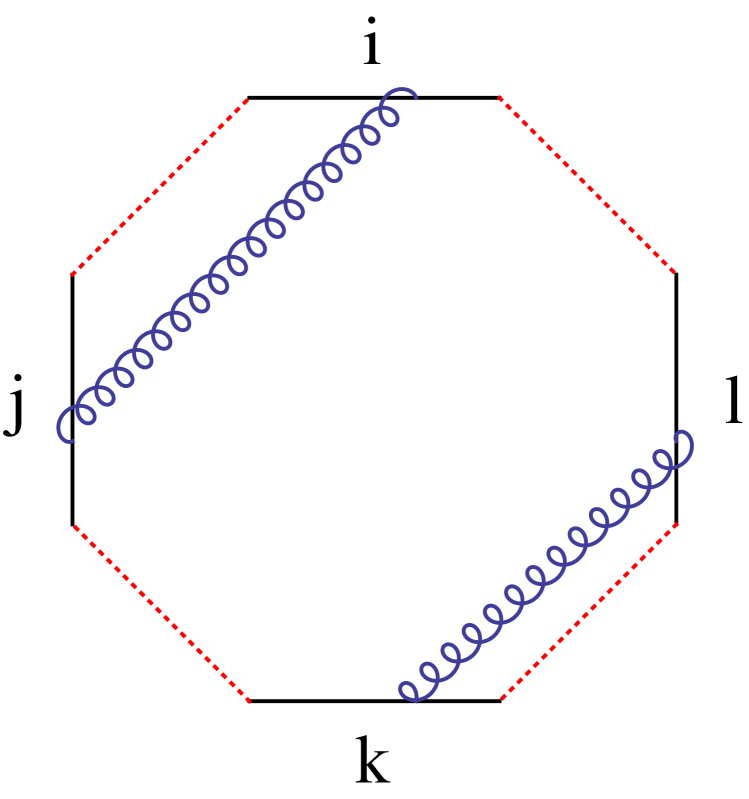
a

Figure 1: 1 Two-gluon diagrams $I_{ijkl}$ given in (24), 1 vertex diagrams $I_{ijk}$ given in (A.2). Dashed lines represent one or more light-like distances.

At two loops there are two types of contributions to the Wilson loop in pure Chern-Simons theory, one from two-gluon diagrams $\langle W_{n}\rangle^{\text{two-gluon}}=\sum I_{ijkl}$ and another one from diagrams involving a three-gluon vertex $\langle W_{n}\rangle^{\text{vertex}}=\sum I_{ijk}$

$$\langle W_{n}\rangle^{\text{CS}}_{\text{2-loop}}=\langle W_{n}\rangle^{\text{two-gluon}}+\langle W_{n}\rangle^{\text{vertex}}\,.$$ (8)

The indices $i,j,k,l$ denote the edges that the propagators attach to, see figure 1 and their expressions are given in appendix A.1, A.2. Contributions from gauge- and ghost-loops cancel in dimensional reduction regularisation Chen:1992ee , for more details see Henn:2010ps .

As explained in Henn:2010ps , the vertex diagrams are divergent in the region of integration where all three propagators approach the same edge (all diagrams with more than one propagator on the same edge vanish identically due to the antisymmetry of the Levi-Civita symbol), and we split them up as in (27)

$$\langle W_{n}\rangle^{\text{vertex}}=\langle W_{n}\rangle^{\text{div}}+\langle W_{n}\rangle^{\text{finite}}\,.$$ (9)

The divergent part can be calculated analytically

$${}\langle W_{n}\rangle^{\text{div}}=-\left(\frac{N}{k}\right)^{2}\left(\frac{\ln(2)}{2}\sum_{i=1}^{n}\frac{(-x_{i,i+2}^{2}\tilde{\mu}^{2})^{2\epsilon}}{2\epsilon}\right)\,.$$

Thus, the function $g_{n}$ in (II) is given by

$$g_{n}(u_{abcd})=\langle W_{n}\rangle^{\text{two-gluon}}+\langle W_{n}\rangle^{\text{finite}}\,.$$ (10)

We evaluate these contributions using a Mathematica program that generates all $n$-point diagrams, performs the index-contractions and numerically integrates the diagrams for randomly generated kinematical configurations, for more details see appendix A.
 
Hexagonal Wilson loop
 
For the hexagonal Wilson loop we evaluated the contributions in (10) for a large set of conformally equivalent and conformally non-equivalent kinematical configurations.

Conformally equivalent configurations must yield the same result, since, by the anomalous conformal Ward identity, the expectation value is constrained to the form (II), and thus the function $g_{n}$ depends only on conformally invariant quantities.

It turns out, that even for kinematical configurations which are not conformally equivalent, the unknown function yields the same constant

$$g_{6}(u_{abcd})=c_{6}-12\ln(2),\quad c_{6}=5.57\pm 0.05\,.$$ (11)

In figure 2 we show the results for the two-gluon and vertex contributions for a continuously deformed kinematical configuration, generated as explained in app. A.3, in order to illustrate, how the different contributions vary while their sum remains constant.

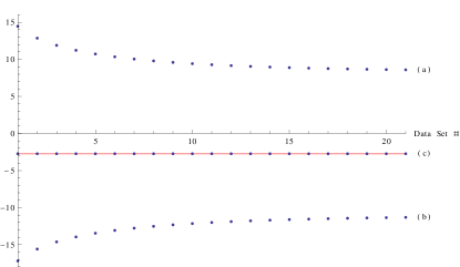
Figure 2: Numerical results for the hexagon $n=6$: $(a)=\langle W_{n}\rangle^{\text{two-gluon}}$, $(b)=\langle W_{n}\rangle^{\text{finite}}$ and their sum $(c)=g_{n}(u_{abcd})$, see (10), for the kinematical points given in A.3. We omit the common factor $\frac{1}{4}\left(\frac{N}{k}\right)^{2}$.

Generalization to $n$ Cusps
 
It turns out that also for $n>6$ the function of conformal cross ratios is just a constant, i.e.

$$g_{n}(u_{abcd})=c_{n}-2n\ln(2)\,.$$ (12)

In figure 3 we show the dependence of the numerical constant $c_{n}$ on the number of cusps $n$ up to $n=14$. Clearly, the constant depends linearly on the number of cusps $n$. It seems reasonable to assume that this dependence holds for all $n$, i.e.

$$c_{n}=a+b\cdot n\,,$$ (13)

which is the line shown in fig. 3 with the parameters $a=6.6\pm 0.1$, $b=-2.028\pm 0.025$. Thus, we expect the Chern-Simons contribution to the $n$-point Wilson loop to be

$$\langle W_{n}\rangle^{\text{CS}} =-\frac{1}{4}\left(\frac{N}{k}\right)^{2}\Bigg{[}2\ln(2)\sum_{i=1}^{n}\frac{(-x_{i,i+2}^{2}\tilde{\mu}^{2})^{2\epsilon}}{2\epsilon}+g_{n}\Bigg{]}$$ (14)

where $g_{n}$ is the constant given by (12) and (13).

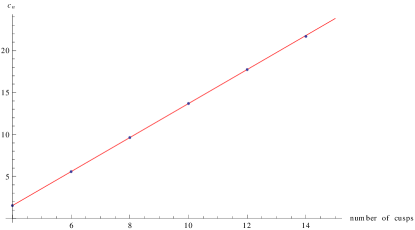
Figure 3: This figure shows the dependence of the constant $c_{n}$ (13) on the number of cusps $n$ of the Wilson loop.

III ABJM theory

In ABJM theory we have two gauge fields $A_{\mu}$, $\hat{A}_{\mu}$ and use the Wilson loop operator proposed in Drukker:2008zx , which is a linear combination of two Wilson loops, each with one of the gauge fields, see also Henn:2010ps . The one-loop contributions are identical to pure Chern Simons theory and cancel each other. Both two-loop contributions yield the same result and thus, it is sufficient to calculate the Wilson loop with the gauge field $A_{\mu}$. In addition to the Chern-Simons contributions (14) we have contributions of bosonic and fermionic matter fields which appear in the one-loop corrected gluon-propagator

$$\langle W_{n}\rangle^{\text{ABJM}}_{\text{2-loop}}=\langle W_{n}\rangle^{\text{CS}}_{\text{2-loop}}+\langle W_{n}\rangle^{\text{matter}}_{\text{2-loop}}\,.$$ (15)

The matter contribution is similar to the one in $\mathcal{N}=4$ SYM Brandhuber:2007yx , since the one-loop corrected propagator calculated in $d$ dimensions Henn:2010ps is

$$G_{\mu\nu}^{(1)}(x) =-\frac{1}{N}\left(\frac{N}{k}\right)^{2}\pi^{2-d}\Gamma\left(\frac{d}{2}-1\right)^{2}\frac{\eta_{\mu\nu}}{(-x^{2})^{d-2}}\,,$$ (16)

which up to two small differences is the tree level $\mathcal{N}=4$ SYM gluon propagator. The first difference is a trivial prefactor, and the second is that since we are at two loops, the power of $1/x^{2}$ is $1-2\epsilon$ here, as opposed to $1-\epsilon$ in the one-loop computation in $\mathcal{N}=4$ SYM. Thus, it is clear that the results will be very similar to the expectation value of the Wilson loop in $\mathcal{N}=4$ SYM.

As in $\mathcal{N}=4$ SYM we have three classes of diagrams shown in figure 4. Diagram 4 vanishes due to the light-likeness of the edges, whereas 4 yields a divergent, and 4 yields a finite contribution.

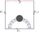
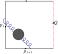
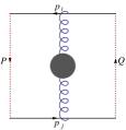
Figure 4: The diagrams involving the one-loop corrected gluon propagator have the same structure as the 1-loop diagrams in $\mathcal{N}=4$ SYM. Dashed lines labelled with $P$ and $Q$ represent one or more light-like distances.

We have Henn:2010ps

$${}\langle W_{n}\rangle^{\text{matter}}_{\text{2-loop}}=\left(\frac{N}{k}\right)^{2}\left((4\pi e^{\gamma_{E}})^{2\epsilon}+\frac{\pi^{2}}{2}\epsilon^{2}\right)\sum_{i>j}I_{ij}$$

where

$$I_{ij}=\frac{1}{2}\int_{0}^{1}ds_{i}\int_{0}^{1}ds_{j}$$ (17)

$$\frac{x^{2}_{i,j+1}+x^{2}_{i+1,j}-x^{2}_{i,j}-x^{2}_{i+1,j+1}}{(-x^{2}_{ij}\bar{s}_{i}\bar{s}_{j}-x^{2}_{i+1,j}s_{i}\bar{s}_{j}-x^{2}_{i,j+1}\bar{s}_{i}s_{j}-x^{2}_{i+1,j+1}s_{i}s_{j})^{d-2}}\,.$$

There are $n$ divergent diagrams $I_{i+1,i}$ of the type shown in fig. 4

$${}I_{i+1,i}=-\frac{1}{8}\frac{(-x_{i,i+2}^{2})^{2\epsilon}}{\epsilon^{2}}$$

and the finite diagrams $I_{ij}$ with $|i-j|\geq 1$, see fig. 4, were solved in Brandhuber:2007yx

$${}I_{ij}=\frac{1}{2}\Big{(} -{\text{Li}_{2}}\left(1-ax_{i,j}^{2}\right)-{\text{Li}_{2}}\left(1-ax_{i+1,j+1}^{2}\right)$$

$$+{\text{Li}_{2}}\left(1-ax_{i,j+1}^{2}\right)+{\text{Li}_{2}}\left(1-ax_{i+1,j}^{2}\right)\Big{)}$$

where

$${}a=\frac{x_{ij}^{2}+x_{i+1,j+1}^{2}-x_{i,j+1}^{2}-x_{i+1,j}^{2}}{x_{ij}^{2}x_{i+1,j+1}^{2}-x_{i,j+1}^{2}x_{i+1,j}^{2}}\,.$$

The sum over all finite diagrams $\sum_{i>j+1}^{n}I_{ij}=\mathcal{F}_{n}^{\text{WL}}$ is related to the well-known finite part of the BDS conjecture Bern:2005iz via $\mathcal{F}_{n}^{\text{WL}}=\mathcal{F}_{n}^{\text{BDS}}-\frac{n}{4}\zeta(2)$, explicitly spelled out in (6) for $n=4$ and $n=6$.

Then, the full matter part reads

$${}\langle W_{n}\rangle^{\text{matter}}_{\text{2-loop}} =-\frac{1}{4}\left(\frac{N}{k}\right)^{2}\Bigg{[}\sum_{i=1}^{n}\frac{(-x_{i,i+2}^{2}\mu^{2}4\pi e^{\gamma_{E}})^{2\epsilon}}{2\epsilon^{2}}$$

$$\qquad\quad\qquad\quad-4\mathcal{F}_{n}^{\text{WL}}+\frac{n}{4}\pi^{2}\Bigg{]}\,.$$ (18)

where we have restored the regularisation scale $\mu$. Taking into account the Chern-Simons result (14), the full result in ABJM theory can be written as

$${}\langle W_{n}\rangle^{\text{ABJM}}_{\text{2-loop}} =\left(\frac{N}{k}\right)^{2}\Bigg{[}-\frac{1}{2}\sum_{i=1}^{n}\frac{(-x_{i,i+2}^{2}\mu^{2}8\pi e^{\gamma_{E}})^{2\epsilon}}{(2\epsilon)^{2}}$$

$$\qquad\qquad\qquad+\mathcal{F}_{n}^{\text{WL}}+r_{n}\Bigg{]}$$ (19)

where $r_{n}=-(\frac{n}{4}\pi^{2}+c_{n}-2n\ln(2)-5n\ln^{2}(2))/4$ and $c_{n}$ is the numerical constant given by (13).

Indeed, this is of the same form as the one-loop result for the Wilson loop in $\mathcal{N}=4$ SYM.

IV Acknowledgements

I would like to thank Marco S. Bianchi, Simon Caron-Huot, Wei-Ming Chen, Livia Ferro, Martin Heinze, Johannes Henn, Yu-tin Huang, Matias Leoni, Andrea Mauri, Silvia Penati, Jan Plefka, Andreas Rodigast, Radu Roiban, Alberto Santambrogio, Theodor Schuster and Sebastian Wuttke for useful discussions, correspondence and comments on the draft. Furthermore, I thank the organisers of the Mathematica summer school, the IGST workshop and conference for hospitality during my stay at the Perimeter Institute, where part of this work was carried out. In particular, I would like to thank Nikolay Gromov and Pedro Viera for their excellent lectures and tutorials on programming with Mathematica, which was extensively used in this project.

Appendix A Two Loop Diagrams

We use the same conventions as in Henn:2010ps , i.e. the metric with $\eta_{\mu\nu}=\text{diag}(1,-1,-1)$ and we define an $n$-sided polygon by $n$ points $x_{i}$ ($i=1,...,n$), with the edge $i$ being the line connecting $x_{i}$ and $x_{i+1}$. Defining

$$p_{i}^{\mu}=x^{\mu}_{i+1}-x^{\mu}_{i}$$ (20)

and parametrising the position $z^{\mu}_{i}$ on edge $i$ with the parameter $s_{i}\in[0,1]$ we have

$$z^{\mu}_{i}(s_{i})=x^{\mu}_{i}+p^{\mu}_{i}s_{i},\quad z_{ij}^{\mu}:=z_{i}^{\mu}-z_{j}^{\mu}$$ (21)

Furthermore, we use the notations

$$\epsilon(p,q,r)=\epsilon_{\mu\nu\rho}p^{\mu}q^{\nu}r^{\rho}\qquad\text{and}\qquad\bar{s}_{i}=1-s_{i}.$$ (22)

We use the Lagrangian of ABJM theory given in Henn:2010ps .

A.1 Two Gluon Diagrams

The contributions from the two-gluon diagrams are all finite and can be written as, see Henn:2010ps ,

$$\langle W_{n}\rangle^{\text{two-gluon}}=\frac{1}{4}\left(\frac{N}{k}\right)^{2}\sum_{i\geq j\geq k\geq l}\left(I_{ij,kl}+I_{il,jk}\right)$$ (23)

where

$$I_{ij,kl}=\int ds_{i,j,k,l}\frac{\epsilon(\dot{z}_{i},\dot{z}_{j},z_{i}-z_{j})}{\left((z_{i}-z_{j})^{2}\right)^{3/2}}\frac{\epsilon(\dot{z}_{k},\dot{z}_{l},z_{k}-z_{l})}{\left((z_{k}-z_{l})^{2}\right)^{3/2}}$$ (24)

and the integration boundaries haven to be chosen according to the path ordering, such that $z(s_{i})>z(s_{j})>z(s_{k})>z(s_{l})$. The diagram vanishes due to the epsilon tensor contractions if the gluon propagator of at least one of the index pairs connects the same or adjacent edges.

As a check of the numerics one can use the factorizing diagrams $I_{i+5,i+3,i+2,i}$, which are just a product of the analytically known one-loop diagrams Bianchi:2011rn .

A.2 Vertex Diagrams

The contribution from the vertex diagrams is calculated in the same way as in Henn:2010ps , but generalized to $n$ points and we find

$$\langle W_{n}\rangle^{\text{vertex}} =-\frac{1}{4}\left(\frac{N}{k}\right)^{2}\left(\pi e^{\gamma_{E}}\right)^{2\epsilon}(1-2\epsilon)$$ (25)

$$\quad\times\frac{1}{4\pi}\sum_{i>j>k}\left(I_{ijk}^{(a)}+I_{ijk}^{(b)}\right)+\mathcal{O}(\epsilon)\,.$$

The indices $i,j,k$ indicate the edges the gluon-propagators connect to and

$${}I^{(a)}_{ijk} =\int ds_{i,j,k},d[\beta]_{3}\epsilon^{\alpha\beta\gamma}\epsilon_{\mu\alpha\sigma}\epsilon_{\nu\beta\lambda}\epsilon_{\rho\gamma\tau}p_{i}^{\mu}p_{j}^{\nu}p_{k}^{\rho}$$

$$\quad\left[\partial_{j}^{\lambda}\Delta\partial_{i}^{\sigma}\partial_{k}^{\tau}\Delta+\partial_{i}^{\sigma}\Delta\partial_{j}^{\lambda}\partial_{k}^{\tau}\Delta+\partial_{k}^{\tau}\Delta\partial_{i}^{\sigma}\partial_{j}^{\lambda}\Delta\right]\Delta^{1-d}$$

$${}I^{(b)}_{ijk} =\int ds_{i,j,k},d[\beta]_{3}\epsilon^{\alpha\beta\gamma}\epsilon_{\mu\alpha\sigma}\epsilon_{\nu\beta\lambda}\epsilon_{\rho\gamma\tau}p_{i}^{\mu}p_{j}^{\nu}p_{k}^{\rho}$$

$$\quad\left[\partial_{i}^{\sigma}\Delta\partial_{j}^{\lambda}\Delta\partial_{k}^{\tau}\Delta\right]\Delta^{-d}(1-d)$$ (26)

where $\partial_{i}^{\mu}=\partial/\partial z_{i,\mu}$ and

$${}\int d[\beta]_{3} =\int_{0}^{1}d\beta_{i,j,k}\delta(\sum_{m}\beta_{m}-1)(\beta_{i}\beta_{j}\beta_{k})^{d/2-2},$$

$${}\Delta =-z_{ij}^{2}\beta_{i}\beta_{j}-z_{ik}^{2}\beta_{i}{\beta}_{k}-z_{kj}^{2}\beta_{k}{\beta}_{j}\,.$$

Integrals with at least two propagators on the same edge (two identical indices $i,j,k$) vanish due to the antisymmetry of $I_{ijk}$ in the indices. Integrals $I^{(a)}_{ijk}$ of the type $i=k+2,j=k+1,k$ are divergent, see Henn:2010ps , all other integrals are finite. The divergent integrals can be split up into a divergent and a finite piece

$$\langle W_{n}\rangle^{\text{vertex}}=\langle W_{n}\rangle^{\text{div}}+\langle W_{n}\rangle^{\text{finite}}\,.$$ (27)

where the divergent piece can be evaluated analytically and reads

$$\langle W_{n}\rangle^{\text{div}}=-\left(\frac{N}{k}\right)^{2}\left(\frac{\ln(2)}{2}\sum_{i=1}^{n}\frac{(-x_{i,i+2}^{2}\mu^{2}\pi e^{\gamma_{E}})^{2\epsilon}}{2\epsilon}\right)\,.$$ (28)

The reamining finite piece is

$$\langle W_{n}\rangle^{\text{finite}}$$ (29)

$${}=-\frac{1}{4}\left(\frac{N}{k}\right)^{2} \left(\frac{1}{4\pi}\sum_{i>j>k}\left(I_{ijk}^{(a,f)}+I_{ijk}^{(b)}\right)-n\,2\ln(2)\right)$$

where $I^{(a,f)},I^{(b)}$ are given by the following expressions for the case $i=k+2,j=k+1,k$. All other cases are treated purely numerically starting from (A.2), i.e. in particular $I^{(a,f)}_{ijk}=I^{(a)}_{ijk}$ in these cases.

For $i=3,j=2,k=1$, after solving two integrations and changing integration parameters to $\beta_{i}=xy,\beta_{j}=\bar{x}y,\beta_{k}=\bar{y}$ (where $\bar{x}=1-x,\bar{y}=1-y$), we have

$$I_{321}^{(a,f)}=-\frac{1}{2}\int_{0}^{1}ds_{j}dxdy\frac{(x\bar{x}\bar{y})^{1/2}}{e^{\prime}f^{\prime}}$$

$$\left(\ln\left(e^{\prime}\frac{x_{13}^{2}}{x_{24}^{2}}+f^{\prime}-\frac{g}{x_{24}^{2}}\right)+\ln\left(e^{\prime}+f^{\prime}\frac{x_{24}^{2}}{x_{13}^{2}}-\frac{g}{x_{13}^{2}}\right)\right)$$

$$+\int_{0}^{1}ds_{j}dxdy\frac{(x\bar{x}\bar{y})^{1/2}}{e^{\prime}f^{\prime}}\left(1+\ln(x\bar{x}\bar{y})+\ln(e^{\prime}f^{\prime})\right)$$

where the last term does not depend on the kinematical quantities and can be further integrated analytically and/or evaluated to high numerical precision. We used the abbreviations

$${}e =-x_{13}^{2}e^{\prime}=-x_{13}^{2}\bar{y}(x+s_{j}\bar{x}),$$

$${}f =-x_{24}^{2}f^{\prime}=-x_{24}^{2}x(\bar{y}+y\bar{s}_{j}\bar{x})$$

$${}g =(x_{13}^{2}+x_{24}^{2}-x_{14}^{2})x\bar{y}\,.$$

Furthermore, after solving two integrations we find

$${}I^{(b)}_{321}=2\int_{0}^{1}dxdyds_{j}(x\bar{y})^{3/2}\bar{x}^{1/2}\frac{(x_{14}^{2}-x_{13}^{2}-x_{24}^{2})}{e^{\prime}f^{\prime}(e+f+g)}\,.$$

These are the expressions we use for the numerical evaluation of the finite parts of the divergent diagrams.

A.3 Generation of kinematical configurations

A set of $n$ light-like ($p_{i}^{2}=0$) vectors $p_{i}^{\mu}$ satisfying momentum conservation $\sum p_{i}^{\mu}=0$ can easily be generated by choosing the $p^{0}_{i}$ components of $n-3$ vectors and the angle $\theta_{i}$ between $p_{i}^{1}=p_{i}^{0}\cos\theta_{i}$, $p_{i}^{2}=p_{i}^{0}\sin\theta_{i}$. The remaining components are then fixed. For $n$ even it is possible to choose configurations, where all non-light-like distances $x_{ij}^{2}$ are space-like. For the numerical evaluation we make use of this type of configurations, such that all integrals are real.

The configurations used for the results shown in fig. 2 are obtained by continuously deforming two angles $\theta_{i}$, leading to conformally non-equivalent kinematical configurations. We use the angles

$$\theta_{i}(a):=\pi\left\{\frac{16}{9}a,\frac{13}{9},\frac{5}{3}a,\frac{13}{8},\frac{19}{14},1\right\}$$ (30)

and choose $p_{i}^{\mu=0}=\{1,-3,4\}$, the remaining components are then fixed. The parameter $a$ is chosen between $a=1$ and $a=1.2$ in steps of $0.01$.

References

- (1) O. Aharony, O. Bergman, D. L. Jafferis and J. Maldacena, “6 superconformal Chern-Simons-matter theories, M2-branes and their gravity duals”, JHEP 0810, 091 (2008), arxiv:0806.1218.
- (2) L. F. Alday and J. M. Maldacena, “Gluon scattering amplitudes at strong coupling”, JHEP 0706, 064 (2007), arxiv:0705.0303.
- (3) J. M. Drummond, G. P. Korchemsky and E. Sokatchev, “Conformal properties of four-gluon planar amplitudes and Wilson loops”, Nucl. Phys. B795, 385 (2008), arxiv:0707.0243.
- (4) A. Brandhuber, P. Heslop and G. Travaglini, “MHV Amplitudes in 4 Super Yang–Mills and Wilson Loops”, Nucl. Phys. B794, 231 (2008), arxiv:0707.1153.
- (5) J. M. Drummond, J. Henn, G. P. Korchemsky and E. Sokatchev, “On planar gluon amplitudes/Wilson loops duality”, Nucl. Phys. B795, 52 (2008), arxiv:0709.2368.
- (6) J. M. Drummond, J. Henn, G. P. Korchemsky and E. Sokatchev, “Dual superconformal symmetry of scattering amplitudes in 4 super-Yang–Mills theory”, Nucl. Phys. B828, 317 (2010), arxiv:0807.1095.
- (7) J. M. Drummond, J. M. Henn and J. Plefka, “Yangian symmetry of scattering amplitudes in 4 super Yang-Mills theory”, JHEP 0905, 046 (2009), arxiv:0902.2987.
- (8) L. F. Alday and R. Roiban, “Scattering Amplitudes, Wilson Loops and the String/Gauge Theory Correspondence”, Phys. Rept. 468, 153 (2008), arxiv:0807.1889.
- (9) J. Henn, “Duality between Wilson loops and gluon amplitudes”, Fortsch.Phys. 57, 729 (2009), arxiv:0903.0522, Based on the author’s Ph.D. thesis at the University Lyon I (France and prepared at LAPTH, Annecy-le-Vieux (France).
- (10) N. Beisert, C. Ahn, L. F. Alday, Z. Bajnok, J. M. Drummond et al., “Review of AdS/CFT Integrability: An Overview”, arxiv:1012.3982, Long author list - awaiting processing.
- (11) J. M. Drummond, J. Henn, G. P. Korchemsky and E. Sokatchev, “The hexagon Wilson loop and the BDS ansatz for the six-gluon amplitude”, Phys. Lett. B662, 456 (2008), arxiv:0712.4138.
- (12) Z. Bern, L. J. Dixon, D. A. Kosower, R. Roiban, M. Spradlin, C. Vergu and A. Volovich, “The Two-Loop Six-Gluon MHV Amplitude in Maximally Supersymmetric Yang-Mills Theory”, Phys. Rev. D78, 045007 (2008), arxiv:0803.1465.
- (13) Z. Bern, L. J. Dixon and V. A. Smirnov, “Iteration of planar amplitudes in maximally supersymmetric Yang-Mills theory at three loops and beyond”, Phys. Rev. D72, 085001 (2005), hep-th/0505205.
- (14) S. Caron-Huot, “Notes on the scattering amplitude / Wilson loop duality”, JHEP 1107, 058 (2011), arxiv:1010.1167.
- (15) L. Mason and D. Skinner, “The Complete Planar S-matrix of N=4 SYM as a Wilson Loop in Twistor Space”, JHEP 1012, 018 (2010), arxiv:1009.2225.
- (16) L. F. Alday, B. Eden, G. P. Korchemsky, J. Maldacena and E. Sokatchev, “From correlation functions to Wilson loops”, arxiv:1007.3243.
- (17) B. Eden, G. P. Korchemsky and E. Sokatchev, “More on the duality correlators/amplitudes”, arxiv:1009.2488.
- (18) B. Eden, P. Heslop, G. P. Korchemsky and E. Sokatchev, “The super-correlator/super-amplitude duality: Part I”, arxiv:1103.3714, * Temporary entry *.
- (19) B. Eden, P. Heslop, G. P. Korchemsky and E. Sokatchev, “The super-correlator/super-amplitude duality: Part II”, arxiv:1103.4353, * Temporary entry *.
- (20) T. Adamo, M. Bullimore, L. Mason and D. Skinner, “A Proof of the Supersymmetric Correlation Function / Wilson Loop Correspondence”, JHEP 1108, 076 (2011), arxiv:1103.4119, * Temporary entry *.
- (21) N. Berkovits and J. Maldacena, “Fermionic T-Duality, Dual Superconformal Symmetry, and the Amplitude/Wilson Loop Connection”, JHEP 0809, 062 (2008), arxiv:0807.3196.
- (22) N. Beisert, R. Ricci, A. A. Tseytlin and M. Wolf, “Dual Superconformal Symmetry from Superstring Integrability”, Phys. Rev. D78, 126004 (2008), arxiv:0807.3228.
- (23) P. A. Grassi, D. Sorokin and L. Wulff, “Simplifying superstring and D-brane actions in superbackground”, JHEP 0908, 060 (2009), arxiv:0903.5407.
- (24) I. Adam, A. Dekel and Y. Oz, “On the fermionic T-duality of the sigma-model”, JHEP 1010, 110 (2010), arxiv:1008.0649.
- (25) I. Adam, A. Dekel and Y. Oz, “On Integrable Backgrounds Self-dual under Fermionic T-duality”, JHEP 0904, 120 (2009), arxiv:0902.3805.
- (26) A. Dekel and Y. Oz, “Self-Duality of Green-Schwarz Sigma-Models”, JHEP 1103, 117 (2011), arxiv:1101.0400.
- (27) I. Bakhmatov, “On x T-duality”, Nucl.Phys. B847, 38 (2011), arxiv:1011.0985.
- (28) I. Bakhmatov, E. O. Colgain and H. Yavartanoo, “Fermionic T-duality in the pp-wave limit”, arxiv:1109.1052, * Temporary entry *.
- (29) T. Bargheer, F. Loebbert and C. Meneghelli, “Symmetries of Tree-level Scattering Amplitudes in N=6 Superconformal Chern-Simons Theory”, arxiv:1003.6120.
- (30) S. Lee, “Yangian Invariant Scattering Amplitudes in Supersymmetric Chern-Simons Theory”, Phys.Rev.Lett. 105, 151603 (2010), arxiv:1007.4772.
- (31) Y.-t. Huang and A. E. Lipstein, “Dual Superconformal Symmetry of N=6 Chern-Simons Theory”, JHEP 1011, 076 (2010), arxiv:1008.0041.
- (32) D. Gang, Y.-t. Huang, E. Koh, S. Lee and A. E. Lipstein, “Tree-level Recursion Relation and Dual Superconformal Symmetry of the ABJM Theory”, JHEP 1103, 116 (2011), arxiv:1012.5032.
- (33) A. E. Lipstein, “Integrability of N = 6 Chern-Simons Theory”, arxiv:1105.3231.
- (34) A. Agarwal, N. Beisert and T. McLoughlin, “Scattering in Mass-Deformed Chern-Simons Models”, JHEP 0906, 045 (2009), arxiv:0812.3367.
- (35) J. M. Henn, J. Plefka and K. Wiegandt, “Light-like polygonal Wilson loops in 3d Chern-Simons and ABJM theory”, JHEP 1008, 032 (2010), arxiv:1004.0226.
- (36) M. S. Bianchi, M. Leoni, A. Mauri, S. Penati, C. A. Ratti et al., “From Correlators to Wilson Loops in Chern-Simons Matter Theories”, JHEP 1106, 118 (2011), arxiv:1103.3675, * Temporary entry *.
- (37) W.-M. Chen and Y.-t. Huang, “Dualities for Loop Amplitudes of N=6 Chern-Simons Matter Theory”, arxiv:1107.2710, * Temporary entry *.
- (38) M. S. Bianchi, M. Leoni, A. Mauri, S. Penati and A. Santambrogio, “Scattering Amplitudes/Wilson Loop Duality In ABJM Theory”, arxiv:1107.3139.
- (39) M. S. Bianchi, M. Leoni, A. Mauri, S. Penati and A. Santambrogio, “Scattering in ABJ theories”, arxiv:1110.0738, * Temporary entry *.
- (40) W. Chen, G. W. Semenoff and Y.-S. Wu, “Two loop analysis of non Abelian Chern-Simons theory”, Phys. Rev. D46, 5521 (1992), hep-th/9209005.
- (41) N. Drukker, J. Plefka and D. Young, “Wilson loops in 3-dimensional N=6 supersymmetric Chern- Simons Theory and their string theory duals”, JHEP 0811, 019 (2008), arxiv:0809.2787.
- (42) K. Wiegandt, “PhD thesis, Humboldt University”.