Mathematical aspects of degressive proportionality

Abstract

We analyze mathematical properties of apportionment functions in the context of allocating seats in the European Parliament. Some exemplary families of such functions are specified and the corresponding allocations of seats among the Member States of the European Union are presented. We show that the constitutional constraints for the apportionment are so strong that the admissible functions lead to rather similar solutions.

1 Introduction

One of the major mathematical approaches to the problem of allocating seats in the European Parliament can be described by the following general scheme. First, one has to choose a concrete characterization of the size of a given Member State $i$ by a number $p_{i}$ (for example, equal to the total number of its inhabitants, citizens, or voters) we call here population, and precisely define by which means these data should be collected and how often they should be updated. Then, one needs to transform these numbers by an allocation (or apportionment) function $A$ belonging to a given family indexed (usually monotonically and continuously) by some parameter $d$, whose range of variability is determined by the requirement that the function fulfills constraints imposed by the treaties: is non-decreasing and degressively proportional.

Additionally, the apportionment function satisfies certain boundary conditions, $A\left(p\right)=m$ and $A\left(P\right)=M$, where the population of the smallest and the largest state equals, respectively, $p$ and $P$, and the smallest and the largest number of seats are predetermined as, respectively, $m$ and $M$. (In the case of the European Parliament these quantities are explicitly bounded by the treaty, $m\geq M_{\min}=6$ and $M\leq M_{\max}=96$.) To obtain integer numbers of seats in the Parliament one has to round the values of the allocation function, e.g., using one of three standard rounding methods (upward, downward or to the nearest integer). Finally, one has to choose the parameter $d$ in such a way that the sum of the seat numbers of all Member States equals the given Parliament size $S$, solving (if possible) in $d$ the equation

$$\sum_{i=1}^{N}\left[A_{d}\left(p_{i}\right)\right]=S\text{ ,}$$ (1)

where $N$ stands for the number of Member States, $p_{i}$ for the population of the $i$-th state ($i=1,\ldots,N$), and $\left[\cdot\right]$ denotes the rounded number. Though usually there is a whole interval of parameters satisfying this requirement, nonetheless, in a generic case, the distribution of seats established in this way is unique. Thus, this technique bears a resemblance to divisor methods in the proportional apportionment problem applied first by Thomas Jefferson in 1792 (Balinski & Young, 1978, Toplak, 2009).

The crucial role in this apportionment scheme plays the notion of degressive proportionality. The principle of degressive proportionality enshrined in the Lisbon Treaty was probably borrowed from the discussions on the taxation rules, where the term has appeared already in the nineteenth century, when many countries introduced income tax for the first time in their history (Young, 1994). It was already included in the debate on the apportionment in the Parliament in late 1980s, but at first, it was a rather vague idea that gradually evolved into a formal legal (and mathematical) term in the report Lamassoure & Severin (2007) adopted by the European Parliament. There were also suggestions to apply this general principle to other parliamentary or quasi-parliamentary bodies like the projected Parliamentary Assembly of the United Nations (Bummel, 2010).

In fact the entire problem of apportionment of seats in the Parliament is mathematically similar (not counting rounding) to the taxation problem, what is illustrated in the table below.

apportionment	taxation
Member States	Tax payers
Population	Income
Seats	Post-tax income
Allocation function	Post-tax income function
Parliament size	Total disposable income
Aeats monotonicity	Income order preservation
Degressivity of seats distribution	Progressivity of tax distribution
Subadditivity of seats distribution	Merging-proofness

In consequence, the similar mathematical tools can be used to solve both of them; see for instance Young (1987), Thomson (2003), Kaminski (2006), Hougaard (2009), Ju & Moreno-Ternero (2011), and Moreno-Ternero (2011), where the authors use the above presented scheme to consider possible parametric solutions of the taxation problem or the dual profit-sharing problem. Of course, the analogy has clear limitations since income and post-tax income are calculated in the same units, whereas population and seats are not. Moreover, money is (at least theoretically) infinitely divisible, while seats are indivisible.

Although quite a novelty in politics, nevertheless, the concept of degressive proportionality is not entirely new in mathematics. It was already analysed in late 1940s under the name of ‘quasi-homogeneity’ by Rosenbaum (1950, Definition 1.4.1), see also Kuczma (2009, p. 480), and since then studied also under the name of ‘subhomogeneity’, see e.g. Burai & Száz (2005). Moreover, an increasing function such that its inverse is degressively proportional (and so it is an allocation function) is called ‘star-shaped’ (with respect to the origin) in the mathematical literature. In other words, the function is degressively proportional if and only if the lines joining points lying below its graph with the origin do not cross the graph. Star-shaped functions were introduced in Bruckner & Ostrow (1962), and since then have been studied in many areas of pure and applied mathematics, see e.g. Ding & Wolfstetter (2009), Dahm (2010). Thus, the results concerning this class of functions can be applied, mutatis mutandis, to degressively proportional functions.

Note that in the original definition of the degressive proportionality formulated in Lamassoure & Severin (2007) it was postulated that this property holds for the number of seats after rounding the values of the allocation function to whole numbers. However, one can show that there exist such distributions of population that there is no solution of the apportionment problem satisfying so understood degressive proportionality (Ramírez González, 2010, Grimmett et al., 2011a). In particular, such difficulty arises in situations where there are a number of Member States having similar populations. Consequently, in Grimmett et al. (2011a) it was recommended to weaken this condition and to amend the definition of degressive proportionality assuming that ‘the ratio between the population and the number of seats of each Member State before rounding to whole numbers must vary in relation to their respective populations in such a way that each Member from a more populous Member State represents more citizens than each Member from a less populous Member State’. This proposal has been recently approved by the The Constitutional Affairs’ Committee of the European Parliament (AFCO). For the detailed mathematical analysis of the original definition of the degressive proportionality, see Łyko et al. (2010), Cegiełka (2011), Florek (2011), Ramírez González et al. (2011), and Serafini (2011).

In this paper we describe several exemplary families of allocation functions and discuss their fundamental properties. Mathematical technicalities collected in Sect. 3-5 can be skipped by more practically oriented readers, who may proceed to Sect. 6, in which general results are applied to the European Parliament.

2 Allocation functions - definition and examples

Before selecting an allocation function $A$ one needs to specify the boundary conditions $m$ and $M$, which denote the number of seats for the smallest and the largest member state, with population $p$ and $P$, respectively. In the case of the European Parliament, the treaty sets the following bounds only: $m\geq M_{\min}=6$ and $M\leq M_{\mathrm{\max}}=96$.

Definition 1.

Let $0<p<P$, $0<m<M$, and $pM<Pm$. We call $A:\left[p,P\right]\rightarrow\left[m,M\right]$ a (degressive) allocation function, if:

1. (monotonicity) $A$ is non-decreasing;

2. (degressive proportionality) $A$ is degressively proportional, i.e. the function $t\rightarrow A\left(t\right)/t$ is non-increasing.

We shall also consider the situation where $P=M=+\infty$, assuming then that $A:\left[p,+\infty\right)\rightarrow\left[m,+\infty\right)$. For the sake of brevity we shall omit the word ‘degressive’ and instead of saying that ‘$A$ is a degressive allocation function’ we shall simply say that ‘$A$ is an allocation function’.

Below, we consider several families of allocation functions fulfilling additionally boundary conditions: $A\left(p\right)=m$ and $A\left(P\right)=M$. Each of them depends on one (free) parameter ($d$) with its range of variability determined by other assumptions imposed on $A$. For instance, in case of the allocation of seats in the Parliament, the parameter $d$ is set by the constraint (1) that the total size of the House is fixed.

Note also that the actual value of the constant $d$ changes from one allocation function to another.

1. base+prop functions - the ‘floor’ version:

   $$A_{1a}(t):=\max\left[m,\;\left(t-P\right)/d+M\right]\text{ ,}$$ (2)

   where $\frac{P}{M}\leq d\leq\frac{P-p}{M-m}$; then the function is convex; and the ‘cup’ version:

   $$A_{1b}\left(t\right):=\min\left[m+\left(t-p\right)/d,\;M\right]\text{ ,}$$ (3)

   where $\frac{p}{m}\leq d\leq\frac{P-p}{M-m}$; in this case the function is concave. Note that not only the choice of the parameter $d$, but also the choice of one of two forms of the base+prop function ($A_{1a}$ or $A_{1b}$) depends on other constraints ($p_{i},i=1,\ldots,N$, and $S$) in (1), see also Sect. 4. Observe further that the base+prop+floor and base+prop+cup functions are in a sense extremal allocation functions satisfying boundary conditions: $A\left(p\right)=m$ and $A\left(P\right)=M$, since it is clear that every such function must fulfill the inequalities:

   $$\max\left[m,\;\left(M/P\right)t\right]\leq A(t)\leq\min\left[\left(m/p\right)t,\;M\right]$$ (4)

   for $t\in\left[p,P\right]$, and thus it is bounded from below by a base+prop+floor function ($d:=P/M$), and from above by a base+prop+cup function ($d:=p/m$).

2. piecewise linear functions:

   $$A_{2a}(t):=\max\left[m+\left(t-p\right)/d,\;\left(M/P\right)t\right]\text{ ,}$$ (5)

   where $\frac{P-p}{M-m}\leq d$; the function is convex; or

   $$A_{2b}(t):=\min\left[\left(m/p\right)t,\;\left(t-P\right)/d+M\right]\text{ ,}$$ (6)

   where $\frac{P-p}{M-m}\leq d$; the function is concave. Again, the choice of one of two forms of the piecewise linear function ($A_{2a}$ or $A_{2b}$) depends on constraints in (1).

3. quadratic (parabolic) functions:

   $$A_{3}\left(t\right):=\left(\frac{t-p}{P-p}\frac{M}{P}+\frac{P-t}{P-p}\frac{m}{p}\right)t-d\left(t-p\right)\left(P-t\right)\text{ .}$$ (7)

   Depending on the system constraints $M,m,P,p$ and the parameter $d$ determined by the total size $S$ of the House, the function is convex or concave. In particular, if

   $$0\leq d-\Theta\leq\frac{\min\left(M-m,m-Mp/P\right)}{\left(P-p\right)^{2}}\text{ ,}$$ (8)

   with $\Theta:=\frac{m/p-M/P}{P-p}$, the function (7) is convex. In the case

   $$0\geq d-\Theta\geq-\frac{\min\left(M-m,mP/p-M\right)}{\left(P-p\right)^{2}}$$ (9)

   the parabolic allocation function is concave.

4. base+power functions:

   $$A_{4}(t):=M\frac{t^{d}-p^{d}}{P^{d}-p^{d}}+m\frac{P^{d}-t^{d}}{P^{d}-p^{d}}\text{ ,}$$ (10)

   where either $0<d\leq 1$ and $\left(M/m-1\right)d\leq\left(P/p\right)^{d}-1$, or $1<d$ and $\left(1-m/M\right)d\leq 1-\left(p/P\right)^{d}$. In the first case the function is concave, in the second convex. In the limiting case ($d\rightarrow 0$) we get a logarithmic function:

   $$A_{l}(t):=\frac{\ln\left(P^{m}/p^{M}\right)+\left(M-m\right)\ln t}{\ln\left(P/p\right)}\text{ ,}$$ (11)

   which is an allocation function, if $M/m-1\leq\ln\left(P/p\right)$.

5. homographic functions:

   $$A_{5}\left(t\right):=\frac{M\left(t/M-d\right)\left(t-p\right)+m\left(t/m-d\right)(P-t)}{\left(P/M-d\right)\left(t-p\right)+\left(p/m-d\right)\left(P-t\right)}\text{ ,}$$ (12)

   where either $d\leq p/M$ or $d\geq P/m$. In the first case the function is concave, in the second convex. In the limiting case ($d\rightarrow\pm\infty$) we get a linear function.

All five families discussed above share a common element: the linear (affine, $\frac{d}{dt}A_{\operatorname*{lin}}\left(t\right)\equiv\operatorname*{const}\geq 0$) function $A_{\operatorname*{lin}}:\left[p,P\right]\rightarrow\left[m,M\right]$ given by the formula

$$A_{\operatorname*{lin}}(t):=M\frac{t-p}{P-p}+m\frac{P-t}{P-p}\text{ .}$$ (13)

On the other hand, if $\frac{d}{dt}\frac{A\left(t\right)}{t}\equiv const\leq 0$, then $A$ must be a quadratic function given by (7) with $d=0$, i.e.,

$$A_{q}\left(t\right):=\left(\frac{t-p}{P-p}\frac{M}{P}+\frac{P-t}{P-p}\frac{m}{p}\right)t\text{ .}$$ (14)

Some of the above solutions were already discussed in the literature, also in the context of the European Parliament.

The base+prop class which seems to lead to the simplest of all these methods was first analysed in Pukelsheim (2007, 2010), see also Martínez-Aroza & Ramírez-González (2008, 2010), and became the basis for the recent proposal, called ‘Cambridge Compromise’, elaborated in January 2011, and discussed later by the Committee on Constitutional Affairs (AFCO) of the European Parliament (Grimmett, 2011, Grimmett et al., 2011a). Here we present this method in the ‘spline’ form, see Martínez-Aroza & Ramírez-González (2008). Likewise, one of the methods of apportionment of seats in the projected Parliamentary Assembly of the United Nations is based on this model (Bummel, 2010, p. 25). Note that, in fact, the composition of the Electoral College that formally elects the President and Vice President of the United States of America also reflects the base+prop scheme, where each state is allocated as many electors as it has Senators (equal base) and Representatives (proportional representation, with at least one seat per state) in the United States Congress. The idea of combining these two approaches to the apportionment problem was first put forward by one of the Founding Fathers of the United States and the future American President, James Madison in 1788 (Madison, 1788).

The quadratic (parabolic) method was proposed and advocated by Ramírez González and his co-workers in a series of papers (Ramírez González, 2004, Ramírez González et al., 2006, Martínez-Aroza & Ramírez-González, 2008, 2010, Ramírez González, 2010).

The methods of apportionment of seats in the European Parliament using base+power functions were also considered by several authors, see Theil & Schrage (1977), Ramírez González et al. (2006), Arndt (2008), Martínez-Aroza & Ramírez-González (2008, 2010), Słomczyński & Życzkowski (2010), Grimmett et al. (2011b) and Moberg (2011). Note that a similar method was proposed for solving the taxation problem already in the nineteenth century by a Dutch economist Arnold Jacob Cohen-Stuart (Cohen-Stuart, 1889). Moreover, the variant of this method (using the square-root function) was also considered in Bummel (2010, p. 27).

As far as we know, out of five families presented above, only the piecewise linear family has not yet been analysed in detail in the European Parliament context, since the homographic functions have been independently studied under the name of projective quotas by Serafini (2011). On the other hand, yet another class of ‘linear-hyperbolic’ functions was used both in the apportionment problem for the European Parliament (Słomczyński & Życzkowski, 2010) as well as in the tax schedule proposed by a Swedish economist Karl Gustav Cassel at the beginning of the twentieth century (Cassel, 1901). Note, that also the proportional apportionment method with minimum and maximum requirements (Balinski & Young, 2001, Martínez-Aroza & Ramírez-González, 2008, p. 133) can be described within this general framework, taking (neither concave nor convex) apportionment function $A$ given by $A(t)=\operatorname*{med}(m,dt,M)$, where $M/P<d<m/p$, and $\operatorname*{med}$ stands for the median value of three.

For a simple and general algorithm of constructing families of allocation functions see Sect. 5.

3 Allocation functions - necessary and sufficient conditions

In this section we present several simple propositions that give necessary and sufficient conditions for a function $A:\left[p,P\right]\rightarrow\left[m,M\right]$ to be a (degressive) allocation function. Almost all these facts belong to mathematical folklore, but we provide short proofs here for the completeness of presentation. First of all, observe that an allocation function needs to be continuous, because, as a non-decreasing function, it can only have jump discontinuities, but this contradicts degressive proportionality.

We start from a simple characterization of allocation functions.

Proposition 1.

$A$ is an allocation function if and only if

$$\frac{A\left(s\right)}{A\left(t\right)}\leq\max\left(1,\frac{s}{t}\right)\text{ ,}$$ (15)

or equivalently

$$\min\left(1,\frac{s}{t}\right)\leq\frac{A\left(s\right)}{A\left(t\right)}$$ (16)

for every $s,t\in\left[p,P\right]$.

See also Peetre (1970, p. 327).

Proof.

Let $s<t$, then (15) is equivalent to $A\left(s\right)/A\left(t\right)\leq 1$. On the other hand for $s>t$ we get $A\left(s\right)/A\left(t\right)\leq s/t$, as desired. ∎

Note that $A$ need not be neither concave nor convex. (Consider, e.g., the allocation function $A:\left[2,8\right]\rightarrow[\sqrt{2}+1/2,2\sqrt{2}+1/8]$ given by $A(t)=\sqrt{t}+1/t$ for $2\leq t\leq 8$, that has an inflection point at $t=4$.) However, if $A$ is an allocation function, then it can be bounded from above by its greatest convex minorant and from below by its least concave majorant. Because of this, it cannot be neither ‘too convex’ nor ‘too concave’.

Corollary 2.

If $A$ is an allocation function, then

$$\frac{1+\sqrt{p/P}}{2}\overline{A}\left(t\right) \leq\frac{t\left(P-p\right)}{P\left(t-p\right)+t\left(P-t\right)}\overline{A}\left(t\right)\leq$$ (17)

$$A\left(t\right) \leq\frac{t\left(P-p\right)}{p\left(P-t\right)+t\left(t-p\right)}\underline{A}\left(t\right)\leq\frac{1+\sqrt{P/p}}{2}\underline{A}\left(t\right)\text{ ,}$$

for each $t\in\left[p,P\right]$, where $\underline{A}$ and $\overline{A}$ denote, respectively, the greatest convex minorant function and the least concave majorant of $A$ (i.e. the largest convex function smaller than $A$ and the smallest concave function larger than $A$).

Proof.

For $t\in\left[p,P\right]$ we have $\overline{A}\left(t\right)=\sup\sum_{i=1}^{n}\lambda_{i}A\left(t_{i}\right)$, where the sum runs over $\lambda_{i}\geq 0$, $t_{i}\in\left[p,P\right]$, $n\in\mathbb{N}$, satisfying $\sum_{i=1}^{n}\lambda_{i}=1$, $\sum_{i=1}^{n}\lambda_{i}t_{i}=t$. From (15) we get $\sum_{i=1}^{n}\lambda_{i}A\left(t_{i}\right)\leq A\left(t\right)\sum_{i=1}^{n}\lambda_{i}\max\left(1,\frac{t_{i}}{t}\right)\leq\frac{2Pt-Pp-t^{2}}{t\left(P-p\right)}A\left(t\right)$. Hence $A\left(t\right)\geq\frac{t\left(P-p\right)}{2Pt-Pp-t^{2}}\overline{A}\left(t\right)\geq\frac{1+\sqrt{p/P}}{2}\overline{A}\left(t\right)$. The proof for the greatest convex minorant is analogous. ∎

The next proposition gives a sufficient condition for a convex or concave non-decreasing function to be an allocation function.

Proposition 3.

If $A$ is non-decreasing, concave and fulfills $A\left(t\right)/t\leq A\left(p\right)/p$ for all $t\in\left[p,P\right]$, or if it is non-decreasing, convex and satisfies $A\left(t\right)/t\geq A\left(P\right)/P$ for all $t\in\left[p,P\right]$, then $A$ is an allocation function. In particular, every concave function $A:\left[0,+\infty\right)\rightarrow\left[0,+\infty\right)$ is an allocation function restricted to any interval $\left[p,P\right]$ for $0<p<P$.

Proof.

In the former case to show that $A$ is degressively proportional, it is enough to observe that $A\left(s\right)/s=A\left(\frac{t-s}{t-p}\cdot p+\frac{s-p}{t-p}\cdot t\right)/s\geq A\left(p\right)\frac{t-s}{\left(t-p\right)s}+A\left(t\right)\frac{s-p}{\left(t-p\right)s}\geq A\left(t\right)/t$ for $s,t\in\left[p,P\right]$, $s<t$, as required. The proof for convex functions is analogous. ∎

In fact, if $A:\left[p,P\right]\rightarrow\left[m,M\right]$ is a restriction of the function defined on the interval $\left[0,P\right]$ such that $A\left(0\right)=0$, then, to get degressive proportionality, it is enough to assume that $A$ is concave on average, i.e., that the function $\left[0,P\right]\ni t\rightarrow a\left(t\right):=\frac{1}{t}\int_{0}^{t}A\left(s\right)ds\in\left[0,M\right]$ is concave, since $A(t)/t=a^{\prime}\left(t\right)+a\left(t\right)/t$ for $0<t\leq P$ and both components are non-increasing functions of $t$ in this case, see Bruckner & Ostrow (1962, Theorem 5).

We call a function $A:\left[p,P\right]\rightarrow\left[m,M\right]$ subadditive if $A\left(s+t\right)\leq A\left(s\right)+A\left(t\right)$ holds for every $s,t,s+t\in\left[p,P\right]$. The subadditivity is the necessary condition for a function being an allocation function, as the next proposition shows. (Analogously, in taxation progressivity of income tax implies its merging-proofness, see Ju & Moreno-Ternero (2011, Corollary 1).)

Proposition 4.

If $A$ is an allocation function, then $A$ is subadditive.

See also Rosenbaum (1950, Theorem 1.4.3) and Hille & Phillips (1957, Theorem 7.2.4).

Proof.

Let $s,t,s+t\in\left[p,P\right]$. From the degressive proportionality we get $A\left(s+t\right)/\left(s+t\right)\leq\min\left(A\left(s\right)/s,A\left(t\right)/t\right)$. Hence $A\left(s+t\right)\leq\left(s+t\right)\left(\frac{s}{s+t}\frac{A\left(s\right)}{s}+\frac{t}{s+t}\frac{A\left(t\right)}{t}\right)=A\left(s\right)+A\left(t\right)$. ∎

The converse implication fails in general, but it holds for convex and non-decreasing functions.

Corollary 5.

If $A:\left[p,+\infty\right)\rightarrow\left[m.+\infty\right)$ is convex and non-decreasing, then $A$ is an allocation function if and only if it is subadditive.

See Rosenbaum (1950, Theorem 1.4.6).

Proof.

According to Proposition 4 it is enough to show that convex, non-decreasing and subadditive function is degressively proportional. Let $p<s<t$. Then $A\left(t\right)\leq\frac{s}{t}A\left(s\right)+\left(1-\frac{s}{t}\right)A\left(s+t\right)\leq\frac{s}{t}A\left(s\right)+\left(1-\frac{s}{t}\right)\left(A\left(s\right)+A\left(t\right)\right)=A\left(s\right)+\left(1-\frac{s}{t}\right)A\left(t\right)$. Hence $A\left(t\right)/t\leq A\left(s\right)/s$, as desired. ∎

4 Allocation functions - concave or convex?

Analyzing possible schemes of allocating seats in the European Parliament several authors consider only concave allocation functions (Martínez-Aroza & Ramírez-González, 2008, 2010). However, as we have seen above, in the class of degressively proportional functions convex and concave functions seem to play similar roles, and both types of functions are represented in each of five basic classes considered.

The affine allocation function (which lies on the border between the concave and the convex realm) can serve as a solution of the apportionment problem if and only if $\sum_{i=1}^{N}A_{\operatorname*{lin}}\left(p_{i}\right)\approx S$. This, however, is only an approximate statement because the effect is influenced by the rounding procedure. Thus, in a concrete case, whether convex or concave functions should be used in the allocation scheme depends approximately on the sign of the expression $\sum_{i=1}^{N}A_{\operatorname*{lin}}\left(p_{i}\right)-S$. Taking into account that

$$\sum\nolimits_{i=1}^{N}A_{\operatorname*{lin}}\left(p_{i}\right)-S=\frac{\left(\left\langle P\right\rangle-p\right)\left(\left\langle M\right\rangle-m\right)N}{P-p}\left(\mu-\rho\right)\text{ ,}$$ (18)

with

$$\rho:=\frac{P-\left\langle P\right\rangle}{\left\langle P\right\rangle-p}$$ (19)

and

$$\mu:=\frac{M-\left\langle M\right\rangle}{\left\langle M\right\rangle-m}\text{ ,}$$ (20)

where $\left\langle P\right\rangle$ and $\left\langle M\right\rangle$ denote, respectively, the mean population of a country and the mean number of seats per country, we see that the solution of the dilemma depends on which of two numbers is greater $\rho$ or $\mu$. If $\rho\geq\mu$ one should use concave functions for resolving the problem, if $\rho\leq\mu$, convex. Since

$$\left(\mu-\rho\right)\left(\left\langle P\right\rangle-p\right)\left(\left\langle M\right\rangle-m\right)N^{2}=$$

$$T\left(M-m\right)-\left(S\left(P-p\right)-N\left(mP-Mp\right)\right)\text{ ,}$$

where $T$ is the total population of the Union, $S$ is the size of the House, and $N$ denotes the number of the Member States, the inequality $\rho\geq\mu$ can be rewritten in the following form affine in $T$, $S$, and $N$:

$$T\leq S\cdot\frac{P-p}{M-m}-N\cdot\frac{mP-Mp}{M-m}\text{ .}$$ (21)

In particular, this implies that any accession of a new state of moderate size (to leave $p$ and $P$ unchanged) to the Union (which means $T,N\uparrow$), keeping ‘constitutional’ parameters ($m$, $M$, $S$) fixed, reduces the probability of finding concave solution of the apportionment problem. Furthermore, the right hand side of (21) is a decreasing function of both $m$ and $M$ (as long as $Nm<S<NM$, which is both a natural and necessary assumption) and an increasing function of $S$. In consequence, seeking concave solutions, one has either to enlarge the size of the House, or to lower the number of seats assigned to the smallest or to the largest Member State (or both).

Note, however, that the treaties define only the minimal ($M_{\min}$) and maximal ($M_{\max}$) numbers of seats in the Parliament, requiring merely that $m:=A\left(p\right)\geq M_{\min}$ and $M:=A\left(P\right)\leq M_{\max}$, as well as the value of $S$. While we have to set the exact values of $m$ and $M$ to start the allocation procedure described in Sect. 1, our choice is formally limited only by these inequalities. Thus, if we believe that the concavity is a desirable feature of an allocation function and it should be possibly incorporated to its definition, we have to agree that the enlargement process will result at some point (defined in fact by the equality in (21)) in lowering the value of $M$ below $M_{\max}$. The only other solution of this problem one can imagine is to introduce an amendment to the treaty either decreasing the minimal number of seats $M_{\min}$ or increasing the total number of seats $S$. However, these two alternatives may be difficult to accept for political reasons, and in this case decreasing the number $M$ seems to be the most feasible solution of the problem within the ‘concave’ realm.

5 Degressive proportionality through logarithmic eyes

We believe that it is sometimes better to analyse allocation functions in logarithmic (log-log) coordinates, since this approach provides us with a number of benefits, namely:

• It is more convenient to plot a graph of population-seats relationship in these coordinates, and so, to compare different allocation methods, since we have more small than large member states in the European Union. NB, this is quite a natural situation from the statistical point of view (‘the larger the fewer’).

• In this setting it is easier to express our assumptions (monotonicity and degressive proportionality) in a uniform way.

• This approach gives us a better framework to analyse certain additional properties of allocation methods.

Definition 2.

Define $L:\left[\ln p,\ln P\right]\rightarrow\left[\ln m,\ln M\right]$ by

$$L(\ln t):=\ln A(t)$$ (22)

for $x\in\left[\ln p,\ln P\right]$. In other words, $L=\ln\circ\,A\circ\exp$ or $A=\exp\circ\,L\circ\ln$.

The choice of a logarithmic base corresponds to the choice of a unit and is not important here.

Proposition 6.

Assume that a function $A:\left[p,P\right]\rightarrow\left[m,M\right]$ is differentiable. Then the following equivalences are true:

$A$ is non-decreasing	$\Leftrightarrow$	$L^{\prime}\geq 0$
$A$ is degressively proportional	$\Leftrightarrow$	$L^{\prime}\leq 1$
$A$ is an allocation function	$\Leftrightarrow$	$0\leq L^{\prime}\leq 1$

.

In particular, the above statement gives us a clear mathematical interpretation of degressive proportionality. Now, our task can be reduced to a search for a function $L:\left[\log p,\log P\right]\rightarrow\left[\log m,\log M\right]$ fulfilling $0\leq L^{\prime}\leq 1$. These can be smoothly realized in a three-fold way:

1. $L$ is affine (i.e. $L^{\prime}$ is constant, i.e. $L^{\prime}\equiv c\in\left[0,1\right]$);

2. $L$ is convex (i.e. $L^{\prime}$ increases from, say, $0$ to $1$) (i.e. $A$ is geometrically convex, see Matkowski (1997));

3. $L$ is concave (i.e. $L^{\prime}$ decreases from, say, $1$ to $0$) (i.e. $A$ is geometrically concave, see Matkowski (1997)).

The first scenario leads to the power function (or in other words, a base+power function with the base $0$) given by $A(t):=b\,t^{d_{\ast}}$, where

$$d_{\ast}:=\left(\ln\left(M/m\right)\right)/\left(\ln\left(P/p\right)\right)$$ (23)

and

$$b:=\left(M-m\right)/(P^{d}-p^{d})=e^{[\left(\ln m\right)\left(\ln P\right)-\left(\ln M\right)\left(\ln p\right)]/\ln\left(P/p\right)}\text{ .}$$ (24)

Rather surprisingly, the distinction between the second and third possibility seems to have a clear interpretation in terms of properties of allocation function $A$, namely, the properties of sub- and superproportionality. The notion of subproportionality and the dual notion of superproportionality were introduced into the decision theory by Daniel Kahneman, a Nobel Prize laureate in economy, and Amos Tversky, a mathematical psychologists, in 1979 (Kahneman & Tversky, 1979) and since then used by many authors, see e.g. Al-Nowaihi & Dhami (2010). Let us recall their definition.

Definition 3.

We say that $A$ is superproportional (subproportional) iff for every $s,t\in\operatorname*{dom}(A)$, $s\leq t$ and $0\leq r\leq 1$ such that $rs,rt\in\operatorname*{dom}(A)$ we have

$$\frac{A(rs)}{A(rt)}\geq\frac{A(s)}{A(t)}\text{ \ \ }\left(\frac{A(rs)}{A(rt)}\leq\frac{A(s)}{A(t)}\right)\text{ .}$$ (25)

Proposition 7.

Let $L:\left[\log p,\log P\right]\rightarrow\left[\log m,\log M\right]$ and $A=\exp\circ L\circ\log$. The following equivalences hold:

• $L$ is convex iff $A$ is superproportional;

• $L$ is concave iff $A$ is subproportional.

Proof.

Note that $A$ is superproportional iff $L(b+a)-L(b)\leq L(c+a)-L(c)$ for $\log p\leq b\leq c\leq c+a\leq\log P$. This property is equivalent to convexity of $L$. The proof of the second equivalence is analogous. ∎

To illustrate this property consider two pairs of member states, Romania/France and Lithuania/Hungary, with the similar population quotient ($s/t\approx 1/3$) and another such configuration: Finland/Portugal and Latvia/Ireland ($s/t\approx 1/2$). In Tab. 1. the values of seat quotients for five methods analysed in Sect. 2 are shown. Note that in all these cases the seat quotient for the ‘smaller’ pair is greater than for the ‘larger’ one.

Table 1: Population ratio (PQ) for exemplary pairs of member states and the corresponding quotients of the number of seats (SQ) in the European Parliament for five classes of allocation functions: $1$ = base+prop, $2$ = piecewise linear, $3$ = parabolic, $4$ = base+power, $5$ = homographic with the rounding to the nearest integer.

ratio	PQ	SQ1	SQ2	SQ3	SQ4	SQ5
RO/FR	0.332	0.376	0.397	0.413	0.418	0.413
LT/HU	0.332	0.556	0.632	0.526	0.526	0.526
Fl/PT	0.503	0.677	0.737	0.684	0.650	0.684
LV/IE	0.503	0.727	0.769	0.727	0.750	0.727

Using other words, a superproportional method leads to the following property of an allocation system (at least before rounding):

The smaller a pair of states is, the larger is the gain

of the small member in the pair over the large one.

Thus, this is in fact a kind of degressive-degressive proportionality. It is easy to show that if an allocation function $A$ is subproportional, then it must be concave, and if it is convex it is necessarily superproportional.

This approach leads also to a simple algorithm for constructing allocation functions, see also Al-Nowaihi & Dhami (2010, Sect. 4). Choose a continuous function $h:\left[p,P\right]\rightarrow\left[0,1\right]$ such that

$$\int_{p}^{P}\frac{h(s)}{s}ds=\ln\left(M/m\right)\text{ .}$$ (26)

Solving the first-order homogeneous linear differential equation of the form

$$A^{\prime}\left(x\right)=\frac{h(x)}{x}A\left(x\right)$$ (27)

with the initial condition $A\left(p\right)=m$ we get the allocation function given by the formula

$$A(t)=m\exp\left(\int_{p}^{t}\frac{h(s)}{s}ds\right)$$ (28)

that fulfills also the final condition $A(P)=M$. In fact, every differentiable allocation function can be obtain in this way. Moreover, $A$ is superproportional (resp. subproportional) iff $h$ is increasing (resp. decreasing), which provides a simple test for checking superproportionality.

To illustrate this technique consider the function $h:\left[p,P\right]\rightarrow\left[0,1\right]$ given by

$$h\left(t\right)=\frac{d}{1+ct^{-d}}\text{ ,}$$ (29)

where the exact value of $c:=\frac{mP^{d}-Mp^{d}}{M-m}$ is determined by the integral condition (26), and we assume additionally that either $d_{1}<d\leq 1$, where

$$d_{1}:=\inf\{0<d<1:\left(M/m-1\right)d\leq\left(P/p\right)^{d}-1\}\text{ ,}$$ (30)

or $1<d<d_{2}$, where

$$d_{2}:=\sup\{d>1:\left(1-m/M\right)d\leq 1-\left(p/P\right)^{d}\}\text{ ,}$$ (31)

in order to ensure that $0\leq h\leq 1$. Applying (28) we get a base+power function $A$ given by (10).

Clearly, the function $h$ defined by (29) is increasing for $c>0$ and decreasing for $c<0$, and so the necessary and sufficient condition for $A$ being superproportional (resp. subproportional) in this case is that $c>0$ (resp. $c<0$) or equivalently $d>d_{\ast}$ (resp. $d<d_{\ast}$), where $d_{\ast}$ is given by (23) and $d_{1}<d_{\ast}<1$.

Summarizing, we have five possible forms of the base+power allocation function:

• concave and subproportional function for $d_{1}<d<d_{\ast}$;

• power function for $d=d_{\ast}$;

• concave and superproportional function for $d_{\ast}<d<1$;

• affine function for $d=1$;

• convex and superproportional function for $1<d<d_{2}$.

Note, however, that in a concrete situation the choice of the value of $d$ is determined by the constraint (1).

6 The European Parliament

For the European Parliament we have the following values of parameters: $p=412\,970$, $M_{\min}=6$, $P=81\,802\,257$, $M_{\max}=96$, $T=501\,103\,425$, $S=751$, and $N=27$. Assuming that the upper and the lower bounds are saturated, $m=M_{\mathrm{min}}$ and $M=M_{\mathrm{max}}$ we obtain $\rho\approx 3.\,485\geq 3.\,126\approx\mu$, so our choice of an allocation function is limited to concave functions. However, it follows from (21) that for the Parliament of size $703$ or less we would have to find the solution of the apportionment problem in the realm of convex functions or otherwise to relax the constraints considering some $M<M_{\max}$. (Due to rounding, this number may be somewhat smaller, cf. Kellermann (2011).) This means also that, in fact, we have currently only about fifty seats to allocate freely besides the linear (or, saying more precisely, affine) distribution.

Analyzing five families of allocation functions and three rounding methods we get fifteen possible solutions for the apportionment problem, see Tab. 2.

Table 2: Fifteen solutions of the apportionment problem for the European Parliament (five classes of allocation functions: $1$ = base+prop, $2$ = piecewise linear, $3$ = parabolic, $4$ = base+power, $5$ = homographic; three rounding methods: $d$ = downwards, $m$ = to the nearest integer, $u$ = upwards); LT = the distribution of seats under the Lisbon Treaty; population figures are taken from the Eurostat website (OJ 22.12.2010 L 338/47).

Country	Population	LT	1d	1m	1u	2d	2m	2u	3d	3m	3u	4d	4m	4u	5d	5m	5u
Germany	81802257	96	96	96	96	96	96	96	96	96	96	96	96	96	96	96	96
France	64714074	74	86	85	83	77	78	78	81	80	80	79	79	79	80	80	80
United Kingdom	62008048	73	82	81	80	74	75	75	78	78	77	76	76	76	77	77	77
Italy	60340328	73	80	79	78	73	73	73	76	76	75	74	74	74	76	76	75
Spain	45989016	54	62	62	61	57	57	58	62	61	60	60	59	59	61	61	60
Poland	38167329	51	53	52	51	49	49	49	53	52	52	52	51	51	53	52	51
Romania	21462186	33	32	32	32	31	31	31	33	33	32	33	33	32	33	33	32
Netherlands	16574989	26	26	26	26	26	26	26	27	27	26	27	27	27	27	27	26
Greece	11305118	22	19	19	19	20	20	20	20	20	20	21	21	20	20	20	20
Belgium	10839905	22	19	19	19	20	20	19	20	20	20	20	20	20	20	20	20
Portugal	10637713	22	18	18	19	19	19	19	19	19	19	20	20	20	20	19	19
Czech Republic	10506813	22	18	18	18	19	19	19	19	19	19	20	20	19	19	19	19
Hungary	10014324	22	17	18	18	19	19	19	19	19	19	19	19	19	19	19	19
Sweden	9340682	20	17	17	17	18	18	18	18	18	18	18	18	18	18	18	18
Austria	8375290	19	15	16	16	17	17	17	16	16	16	17	17	17	17	17	17
Bulgaria	7563710	18	14	15	15	16	16	16	15	15	15	16	16	16	15	15	15
Denmark	5534738	13	12	12	13	14	14	14	13	13	13	13	13	13	13	13	13
Slovakia	5424925	13	12	12	12	14	14	14	12	13	13	13	13	13	13	13	13
Finland	5351427	13	12	12	12	14	14	14	12	13	13	13	13	13	12	13	13
Ireland	4467854	12	11	11	11	13	13	13	11	11	12	12	12	12	11	11	12
Lithuania	3329039	12	9	10	10	12	12	11	10	10	10	10	10	11	10	10	10
Latvia	2248374	9	8	8	9	11	10	10	8	8	9	9	9	9	8	8	9
Slovenia	2046976	8	8	8	8	10	10	10	8	8	9	8	9	9	8	8	9
Estonia	1340127	6	7	7	8	10	9	9	7	7	8	7	7	8	7	7	8
Cyprus	803147	6	6	6	7	9	9	9	6	7	7	6	7	7	6	7	7
Luxembourg	502066	6	6	6	7	7	7	8	6	6	7	6	6	7	6	6	7
Malta	412970	6	6	6	6	6	6	6	6	6	6	6	6	6	6	6	6
EU-27	501103425	751	751	751	751	751	751	751	751	751	751	751	751	751	751	751	751

Observe that all these solutions are quite similar, which is a consequence of the fact that our choice is limited by two factors: the predetermined shape of the graph of an allocation function, and the fact that more than ninety percent of seats are in a sense distributed in advance. More precisely, the results for the parabolic, base+power, and homographic allocation functions are almost identical, whereas the choice of the base+prop functions is advantageous for large countries, and the choice of the piecewise linear functions seems to be beneficial for small countries.

The influence of the choice of a rounding method on the distribution of seats is a non-trivial mathematical problem even for proportional apportionment (Balinski & Young, 2001, Janson, 2011), where it was proven that, statistically, the rounding downwards is more often advantageous for large countries and the rounding upwards for small countries, see Schuster et al. (2003), Drton & Schwingenschlögl (2005), Schwingenschlögl (2008). In the case of the European Parliament one can observe a similar effect for the base+linear, parabolic, base+power and homographic functions, where the rounding downwards is the best possibility and the rounding upwards is the worst for large countries (from the Netherlands to France), whereas for small countries (from Malta to Austria) the situation is reversed. However, for the piecewise linear class we find completely different pattern, and so it is not clear to what extent this rule applies to degressively proportional apportionment.

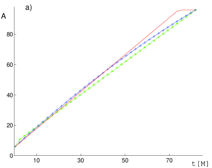
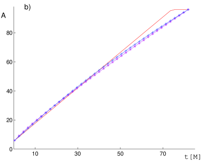
Figure 1: Allocation functions applied to the European Parliament: panel a) concave base+prop function (3) (solid line), piecewise linear function (6) ($\ast$), and parabolic function (7) ($+$); panel b) function (3) drawn as a reference solid line, base+power function (10) ($\ast$), and homographic function (12) ($+$). The argument $t$ denotes the population of a state in millions, while $A$ is scaled to determine the corresponding number of seats in the Parliament consisting of $S=751$ members with the constraints $m=6$ and $M=96$ seats.

As regards superproportionality, the base+prop method is superproportional in the ‘affine’ part of its domain, i.e. for all countries but the largest one, the piecewise linear method for all countries but two smallest ones, and the parabolic (resp. homographic) method are superproportional for small and medium countries and subproportional for large five (resp. six) ones.

The only one of the five methods that is superproportional in the whole domain $\left[p,P\right]$ is the base+power method. In fact, we showed that this method is superproportional as long as $d>d_{\ast}$, where $d_{\ast}$ is given by (23). In the analysed case $d_{\ast}\approx 0.\,524$ and $d=0.865$, $0.894$, $0.922$ depending on the rounding method chosen, so the condition is clearly fulfilled. Though it is not known whether superproportionality is what the authors of the Lisbon Treaty really intended, when they formulated the ‘degressive proportionality’ rule, we think that it is worth to realize that the base+power method fulfills it for all pairs, whereas the other methods can violate it for some countries. Thus base+power method is in a sense more degressively proportional, or one can say degressively proportional in more perfect way, than other methods analysed above. Incidentally, the base+power solution with $c=0.5$ (the square root) results (with downward rounding) in a round number of $1000$ members of the Parliament.

In Grimmett et al. (2011a) the authors decided to select the method called ‘Cambridge Compromise’, which is in this case equivalent to the base+prop method (as defined above) with the rounding to the nearest integer, mainly because of its obvious simplicity. However, this solution has been criticized for being ‘not enough degressively proportional’ (Moberg, 2011) and departing too much from the status quo. In Grimmett et al. (2011b) the solution very similar to the base+power method discussed here is considered ‘as a step along a continuous transition from the negotiated status quo composition to the constitutionally principled Cambridge Compromise.’ (Indeed this method is closest to the status quo out of all methods analyzed in Tab. 2.) The crucial point in these discussions seems to be the meaning of the term ‘degressive proportionality’. Is it only a lame form of (pure) proportionality, as it was actually suggested in Grimmett et al. (2011b) or is it a separate notion that requires distinct mathematical and political solutions, as Moberg (2011) claims? In this paper we have tried to shed new light on this debate, analyzing mathematical properties of degressively proportional allocation functions and indicating the differences between various classes of such functions.

If we are looking for a degressively proportional (resp. degressively proportional and superproportional) and increasing function, in the log-log realm we have to find a function (resp. convex function) with the derivative contained between $0$ and $1$. Adding to this, three constraints related to the minimum and maximum number of seats and to the size of the House, we see that our choice is in fact very limited and all the solution satisfying these conditions must look quite similar – see Fig. 2.

The key possibility to vary the allocation schemes considerably is to change the number $M$ of the seats allotted to the largest member state. As specified in the Treaty of Lisbon the upper bound reads $M_{\mathrm{\max}}=96$, but this bound needs not to be saturated and one may also take $M<M_{\mathrm{\max}}$. By doing so, one introduces more freedom into the space of possible solutions, as more seats can be allotted besides the affine distribution.

Note also that by extending the Union and keeping the number $M$ fixed (which is, however, in the ‘concave realm’, doable only up to a certain total population of the Union), the seats for the new member states are donated by all but the largest state. If any further enlargement of the Union was performed according to this scheme, the ratio of the seats in the European Parliament allocated to the largest state would remain constant. In consequence, as the number $N$ of the member states was increased, the voting power of the largest state in the European Union would grow.

These arguments show that the choice of the number $M$ selected to design an allocation system is crucial. The issue: under what conditions the constraint $M=M_{\mathrm{\max}}$ should be relaxed seems to be equally important as the choice of the actual form of allocation function. As regards the latter, it is rather difficult task to distinguish in practice one of them. From an academic perspective, however, it would be interesting to base the solution of the ‘degressive’ allocation problem on an axiomatic approach, possibly considering some additional properties of allocation functions as concavity and superproportionality.

Acknowledgements. It is a pleasure to thank Geoffrey Grimmett and Friedrich Pukelsheim for inviting us to the Cambridge Apportionment Meeting, where this work was initiated, and all the participants of this meeting for fruitful and stimulating discussions, as well as Axel Moberg for providing us with an earlier version of his paper and for interesting correspondence.

References

- Al-Nowaihi & Dhami (2010) Al-Nowaihi, A., & Dhami, S. (2010). A value function that explains the magnitude and sign effects. Economics Letters, 105, 224–229.
- Arndt (2008) Arndt, F. (2008). Ausrechnen statt aushandeln: Rationalitätsgewinne durch ein formalisiertes Modell für die Bestimmung der Zusammensetzung des Europäischen Parlaments (with English summary). Zeitschrift für ausländisches öffentliches Recht und Völkerrecht - Heidelberg Journal of International Law, 68, 247–279.
- Balinski & Young (1978) Balinski, M. L. & Young, H. P. (1978). The Jefferson method of apportionment, SIAM Review, 20, 278–284.
- Balinski & Young (2001) Balinski, M. L. & Young, H. P. (2001). Fair Representation. Meeting the Ideal of One Man, One Vote. (2nd ed.). Washington: Brookings Institution Press.
- Bruckner & Ostrow (1962) Bruckner, A. M., & Ostrow, E. (1962). Some function classes related to the class of convex functions. Pacific Journal of Mathematics, 12, 1203–1215.
- Bummel (2010) Bummel, A. (2010). The Composition of a Parliamentary Assembly at the United Nations. Berlin: Committee for a Democratic U.N., Background Paper no. 3.
- Burai & Száz (2005) Burai, P., & Száz, A. (2005). Relationships between homogeneity, subadditivity and convex properties. Univerzitet u Beogradu. Publikacije Elektrotehničkog Fakulteta. Serija Matematika, 16, 77–87.
- Cassel (1901) Cassel, K. G. (1901). The theory of progressive taxation. The Economic Journal, 11, 481–491.
- Cegiełka (2011) Cegiełka, K. (2011). Degressive proportionality in the European Parliament. arXiv:1109.2859v1 [physics.soc-ph].
- Cohen-Stuart (1889) Cohen-Stuart, A. J. (1889). Bijdrage tot de Theorie der progressieve Inkomstenbelastning. Den Haag: Martinus Nijhoff.
- Dahm (2010) Dahm, M. (2010). Free mobility and taste-homogeneity of jurisdiction structures. International Journal of Game Theory, 39, 250-272.
- Ding & Wolfstetter (2009) Ding, W., & Wolfstetter, E. (2009). Prizes and Lemons: Procurement of Innovation under Imperfect Commitment. Berlin: Governance and the Efficiency of Economic Systems Discussion Paper No. 262.
- Drton & Schwingenschlögl (2005) Drton, M., & Schwingenschlögl, U. (2005). Asymptotic seat bias formulas. Metrika, 62, 23–31.
- Florek (2011) Florek, J. (2011). A numerical method to determine a degressive proportional distribution of seats in the European Parliament. Mathematical Social Sciences, This issue.
- Grimmett (2011) Grimmett, G. (2011). European apportionment via the Cambridge Compromise. Mathematical Social Sciences, This issue.
- Grimmett et al. (2011a) Grimmett, G., with Laslier, J.-F., Pukelsheim, F., Ramírez-González, V., Rose, R., Słomczyński, W., Zachariasen, M., & Życzkowski, K. (2011). The allocation between the EU Member States of the seats in the European Parliament. European Parliament Studies, PE 432.760.
- Grimmett et al. (2011b) Grimmett, G., Oelbermann, K-F., & Pukelsheim, F. (2011). A power-weighted variant of the EU27 Cambridge Compromise. Mathematical Social Sciences, This issue.
- Janson (2011) Janson, S. (2011). Asymptotic bias of some election methods. arXiv:1110.6369v1 [math.PR].
- Ju & Moreno-Ternero (2011) Ju, B.-G., & Moreno-Ternero, J. D. (2011). Progressive and merging-proof taxation. International Journal of Game Theory, 40, 43–62.
- Hille & Phillips (1957) Hille, E., & Phillips, R. S. (1957). Functional Analysis and Semi-Groups. New York: Amer. Math. Soc. Coll. Publ., Vol. 31.
- Hougaard (2009) Hougaard, J. L. (2009). Introduction to Allocation Rules. Berlin: Springer-Verlag.
- Kahneman & Tversky (1979) Kahneman, D., & Tversky, A. (1979). Prospect theory: An tnalysis of decision under risk. Econometrica, 47, 263–292.
- Kaminski (2006) Kaminski, M. K. (2006). Parametric rationing methods. Games and Economic Behavior, 54, 115–133.
- Kellermann (2011) Kellermann, T. (2011). The minimum-based procedure: A principled way to allocate seats in the European Parliament. Mathematical Social Sciences, This issue.
- Kuczma (2009) Kuczma, M. (2009). An Introduction to the Theory of Functional Equations and Inequalities. (2nd ed., ed. by A. Gilányi). Basel: Birkhäuser.
- Lamassoure & Severin (2007) Lamassoure, A., & Severin, A. (2007). European Parliament Resolution on ‘Proposal to amend the Treaty provisions concerning the composition of the European Parliament’ adopted on 11 October 2007 (INI/2007/2169).
- Łyko et al. (2010) Łyko, J., Cegiełka, K., Dniestrzański, P., & Misztal, A. (2010). Demographic changes and principles of the fair division. International Journal of Social Sciences and Humanity Studies, 2, 63–72.
- Madison (1788) Madison, J. (1788). Federalist Paper No. 39. The Conformity of the Plan to Republican Principles. The Independent Journal, January 18, 1788.
- Martínez-Aroza & Ramírez-González (2008) Martínez-Aroza, J., & Ramírez-González, V. (2008). Several methods for degressively proportional allotments. A case study. Mathematical and Computer Modelling, 48, 1439–1445.
- Martínez-Aroza & Ramírez-González (2010) Martínez-Aroza, J., & Ramírez-González, V. (2010). Comparative analysis for several methods for determining the composition of the European Parliament. In M. Cichocki, & K. Życzkowski (Eds.), Institutional Design and Voting Power in the European Union (pp. 255-267). London: Ashgate.
- Matkowski (1997) Matkowski, J. (1997). Iteration groups with generalized convex and concave elements. Grazer Mathematische Berichte, 334, 199–216.
- Moberg (2011) Moberg, A. (2011). EP seats: The politics behind the math. Mathematical Social Sciences, This issue.
- Moreno-Ternero (2011) Moreno-Ternero, J. D. (2011). Voting over piece-wise linear tax methods. Journal of Mathematical Economics, 47, 29–36.
- Peetre (1970) Peetre, J. (1970). Concave majorants of positive functions. Mathematica Academiae Scientiarum Hungaricae, 21, 327–333.
- Pukelsheim (2007) Pukelsheim, F. (2007). A Parliament of Degressive Representativeness? Institut für Mathematik, Universität Augsburg, Preprint Nr. 015/2007.
- Pukelsheim (2010) Pukelsheim, F. (2010). Putting citizens first: Representation and power in the European Union. In M. Cichocki, & K. Życzkowski (Eds.), Institutional Design and Voting Power in the European Union (pp. 235-253). London: Ashgate.
- Ramírez González (2004) Ramírez González, V. (2004). Some Guidelines for an Electoral European System. Workshop on Institutions and Voting Rules in the European Constitution. Seville, 10-12 December 2004.
- Ramírez González (2010) Ramírez-González, V. (2010). Degressive proportionality. Composition of the European Parliament. The parabolic method. In M. Cichocki, & K. Życzkowski (Eds.), Institutional Design and Voting Power in the European Union (pp. 215-234). London: Ashgate.
- Ramírez González et al. (2006) Ramírez González, V., Palomares Bautista, A., & Márquez García, M. (2006). Degressively proportional methods for the allotment of the European Parliament seats amongst the EU member states. In B. Simeone, & F. Pukelsheim (Eds.), Mathematics and Democracy. Recent advances in Voting Systems and Collective Choice (pp. 205-220). Berlin: Springer Verlag.
- Ramírez González et al. (2011) Ramírez González, V., Palomares Bautista, A., & Márquez García, M. (2011). Spline methods for degressive proportionality in the composition of European Parliament. Mathematical Social Sciences, This issue.
- Rosenbaum (1950) Rosenbaum, R. A. (1950). Sub-additive functions. Duke Mathematical Journal, 17, 227–247.
- Schuster et al. (2003) Schuster, K., Pukelsheim, F., Drton, M., & Draper, N. R. (2003). Seat biases of apportionment methods for proportional representation. Electoral Studies, 22, 651–676.
- Schwingenschlögl (2008) Schwingenschlögl, U. (2008). Asymptotic equivalence of seat bias models. Statistical Papers, 49, 191–200.
- Serafini (2011) Serafini, P. (2011). Allocation of the EU Parliament seats via integer linear programming and revised quotas. Mathematical Social Sciences, This issue.
- Słomczyński & Życzkowski (2010) Słomczyński, W., & Życzkowski K. (2010). On bounds for the allocation of seats in the European Parliament. In M. Cichocki, & K. Życzkowski (Eds.), Institutional Design and Voting Power in the European Union (pp. 269-281). London: Ashgate.
- Theil & Schrage (1977) Theil, H., & Schrage, L. (1977). The apportionment problem and the European Parliament. European Economic Review, 9, 247–263.
- Thomson (2003) Thomson, W. (2003). Axiomatic and game-theoretic analysis of bankruptcy and taxation problems: a survey. Mathematical Social Sciences, 45, 249–297.
- Toplak (2009) Toplak, J. (2009). Equal voting weight of all: Finally ‘One Person, One Vote’ from Hawaii to Maine? Temple Law Review, 81, 123–176.
- Young (1987) Young, P. (1987). On dividing an amount according to individual claims or liabilities. Mathematics of Operations Research, 12, 398–414.
- Young (1994) Young, P. (1994). Equity. Princeton: Princeton University Press.