Quantum Noise Measurement of a Carbon Nanotube Quantum Dot in the Kondo Regime

Abstract

The current emission noise of a carbon nanotube quantum dot in the Kondo regime is measured at frequencies $\nu$ of the order or higher than the frequency associated with the Kondo effect $k_{B}T_{K}/h$, with $T_{K}$ the Kondo temperature. The carbon nanotube is coupled via an on-chip resonant circuit to a quantum noise detector, a superconductor-insulator-superconductor junction. We find for $h\nu\approx k_{B}T_{K}$ a Kondo effect related singularity at a voltage bias $eV\approx h\nu$, and a strong reduction of this singularity for $h\nu\approx 3k_{B}T_{K}$, in good agreement with theory. Our experiment constitutes a new original tool for the investigation of the non-equilibrium dynamics of many-body phenomena in nanoscale devices.

How does a correlated quantum system react when probed at frequencies comparable to its intrinsic energy scales ? Thanks to progress in on-chip detection of high frequency electronic properties, exploring the non-equilibrium fast dynamics of correlated nanosystems is now accessible though delicate. In this respect, the Kondo effect in quantum dots is a model many-body system, where the spin of the dot is screened by the contacts’ conduction electrons below the Kondo temperature $T_{K}$ goldhaber98 ; cronenwett98 ; nigard00 . The Kondo effect can then be probed at a single spin level and in out-of-equilibrium situations. It leads to a strong increase of the conductance of the quantum dot at zero bias due to the opening of a spin degenerate conducting channel, the transmission of which can reach unity. This effect has been extensively studied by transport and noise experiments in the low frequency limit meir02 ; sela06 ; golub06 ; gogolin06 ; mora08 ; delattre09 ; zarchin08 ; yamauchi11 . However the noise in the high frequency limit has not been explored experimentally despite the fact that it allows to probe the system at frequencies of the order or smaller than $k_{B}T_{K}/h$ characteristic of the Kondo effect nordlander99 . In this letter we present the first high frequency noise measurements of a carbon nanotube quantum dot in the Kondo regime. We find for $h\nu\approx k_{B}T_{K}$ a Kondo effect related singularity at a voltage bias $eV\approx h\nu$, and a strong reduction of it for $h\nu\approx 3k_{B}T_{K}$. These results are compared to recent theoretical predictions.

The high frequency current fluctuations are measured by coupling the carbon nanotube (CNT) to a quantum noise detector, a Superconductor-Insulator-Superconductor (SIS) junction, via a superconducting resonant circuit (see figure 1a). This allows us to probe the emission noise of the CNT at the resonance frequencies of the coupling circuit (29.5 GHz and 78 GHz) by measuring the photo-assisted tunneling current through the detector basset10 . The probed sample consists of two coupled coplanar transmission lines. One line is connected to the ground plane via a carbon nanotube and the other via a superconducting tunnel junction of size $240\times 150$ nm² (figure 1). Each transmission line consists of two sections of same length $l$ but different widths, thus different characteristic impedances $Z_{1}\approx 110\Omega$ and $Z_{2}\approx 25\Omega$ (figure 1a). Due to the impedance mismatch, the transmission line acts as a quarter wavelength resonator, with resonances at frequencies $\nu_{n}=nv/4l=n\nu_{1}$, with $v$ the propagation velocity and $n$ an odd integer basset10 . The two transmission lines are close to one another to provide a good coupling at resonance and are terminated by on-chip Pd resistors. The junction has a SQUID geometry to tune its critical current with a magnetic flux. The carbon nanotube (CNT) is first grown by chemical vapor deposition on an oxidized undoped silicon wafer kasumov07 . An individual CNT is located relative to predefined markers and contacted to palladium leads using electron-beam lithography. The junction and the resonator are then fabricated in aluminum (superconducting gap $\Delta=182\mu$eV). A nearby side-gate allows to change the electrostatic state of the nanotube. The system is thermally anchored to the cold finger of a dilution refrigerator of base temperature 20 mK and measured through low-pass filtered lines with a standard low frequency lock-in amplifier technique.

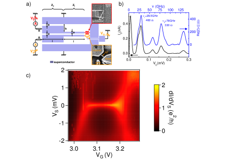
Figure 1: (a) Sketch of the sample: a carbon nanotube (bottom electron microscope picture) is coupled to a superconductor-insulator-superconductor (SIS) junction (top electron microscope picture), used as a quantum detector, by a superconducting resonant circuit. This circuit is constituted by two transmission lines, placed close to one another, made of aluminum and terminated by on-chip Pd resistors. The SIS junction is fabricated by shadow angle evaporation. The carbon nanotube is CVD grown, connected with Palladium contacts and side-gated. (b) Lower curve : $I(V)$ of the detector in the subgap region. Upper curve: The real part of the impedance seen by the detector exhibits several resonances. (c) Differential conductance $dI/dV_{S}$ of the carbon nanotube as a function of voltage bias $V_{S}$ and gate voltage $V_{G}$. It exhibits a Kondo ridge for gate voltage between 3.05 and 3.20 V with an increase of conductance at zero bias.

To characterize the CNT-quantum dot, we first measure its differential conductance $dI/dV_{S}$ as a function of dc bias voltage $V_{S}$ and gate voltage $V_{G}$ (figure 1c). For a gate voltage between 3.05 and 3.2V the CNT’s conductance at zero bias strongly increases, a signature of the Kondo effect. The half width at half maximum (HWHM) of the Kondo ridge yields the Kondo temperature $T_{K}=1.4$K in the center of the ridge goldhaber98 . This value is also consistent with the temperature dependence of the zero bias conductance. The Kondo temperature is related to the charging energy $U$ of the CNT quantum dot, the coupling $\Gamma$ to the electrodes and the position $\epsilon$ of the energy level measured from the center of the Kondo ridge, according to Bethe-Ansatz tsvelick83 ; bickers87 :

$$T_{K}=\sqrt{U\Gamma/2}\exp\left[-\frac{\pi}{8U\Gamma}|4\epsilon^{2}-U^{2}|\right]\;.$$ (1)

From $U=2.5$meV, deduced from the size of the Coulomb diamond, and $T_{K}=1.4$K, we obtain $\Gamma=0.51$meV. The asymmetry $A=(\Gamma_{L}-\Gamma_{R})/(\Gamma_{L}+\Gamma_{R})=0.67$ of the contacts is deduced from the zero bias conductance.

To characterize the superconducting resonant circuit which couples the detector junction to the CNT, we measure the subgap $I(V)$ characteristic of the junction which depends on the impedance of its electromagnetic environment ingold92 . In the case of a superconducting transmission line resonator basset10 ; holst94 , resonances appear in the subgap region $V_{D}<2\Delta/e$ due to the excitation of the resonator modes by the ac Josephson effect barone82 . These resonances are related to the real part of the impedance $Z(\nu)$ seen by the junction:

$$I(V_{D})=Re[Z(2eV_{D}/h)]\,I_{C}^{2}/2V_{D}\;,$$ (2)

with $I_{C}=\pi\Delta/(2eR_{N})$ the critical current barone82 , $R_{N}=28.6k\Omega$ the normal state resistance of the junction and $\Delta$ the superconducting gap of the electrodes. Equation 2 accounts for the effect of the electromagnetic environment on the tunneling of Cooper pairs through the Josephson junction ingold92 . Figure 1b shows the $I(V)$ of the junction in the subgap region for $I_{C}$ maximized with magnetic flux. The subgap resonances thus yield via equation 2 $Re[Z(\nu)]$ (Fig. 1b) which is peaked at frequencies $\nu_{1}=29.5$ and $\nu_{3}=78$GHz. Using the height and width of the resonance peaks of $Re[Z(\nu)]$, we infer the coupling between the junction and the CNT basset10 . We then translate a photo-assisted tunneling (PAT) quasi-particles current measurement into a current emission noise measurement for the frequencies $\nu_{1}$ and $\nu_{3}$. The ratio $r_{n}$ between the measured PAT current through the detector and the current emission noise of the CNT at a given resonance frequency is estimated as follows. $r_{n}$ is given at the resonant frequency $\nu_{n}$ by $e^{2}|Z_{t}(\nu_{n})|^{2}\delta\nu_{n}/(h\nu_{n})^{2}I_{QP,0}(V_{D}+\frac{h\nu_{n}}{e})$ with $Z_{t}$ the transimpedance of the coupling circuit, defined as the ratio between the voltage fluctuations across the detector and the current fluctuations through the source, $\delta\nu_{n}$ the width of the resonance peak and $I_{QP,0}(V_{D})$ the I-V characteristic of the detector basset10 . This value has been calibrated in a previous experiment with the same design as the one used in the present work basset10 . $r_{n}$ is then calculated using the ratio of the calibrated sample corrected according to the square area under the corresponding peak of $Re[Z(\nu)]$ (figure 1b), the value of $\nu_{n}$, the superconducting gap and the tunnel resistance of the detector junction.

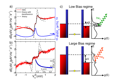
Figure 2: (a) Derivative of the current noise and differential conductance of the CNT versus $V_{S}$ in the center of the Kondo ridge. Left axis : measured $dS_{I}/dV_{S}$ (in red) at $29.5$GHz as a function of bias voltage $V_{S}$. The black solid line corresponds to the calculated $dS_{I}/dV_{S}$ with a fitted decoherence rate incorporating both intrinsic and extrinsic decoherence (see text), while the dashed line is the theoretical prediction with the intrinsic decoherence rate. Right axis : Differential conductance $dI/dV_{S}$ of the CNT in units of $e^{2}/h$. (b) Same data at $78$GHz. Inset : measured conductance, symmetrized with respect to the bias voltage, in units of $e^{2}/h$. The black solid line correspond the the FRG calculation of the conductance with the same fitted decoherence rate as the one used for the noise measurements. (c) Schematic picture of a quantum dot in the out-of-equilibrium Kondo regime together with the density of states for two distinct bias voltages. When the quantum dot is voltage biased, the Kondo resonance splits in two with a splitting given by the applied bias voltage. This leads to an increase of the emission at frequency $eV_{S}=h\nu$. The amplitude of the resonance peaks, and thus the emission noise at $eV_{S}=h\nu$, can be reduced by decoherence effects induced by the applied bias voltage.

To measure the quantum noise of the CNT, we modulate its bias voltage $V_{S}$ and monitor the modulated part of the PAT current through the detector for a given detector bias voltage $V_{D}$. $V_{D}$ selects the frequency range of the measurement basset10 . We have thus access to the derivative of the PAT current versus CNT bias voltage $dI_{PAT}/dV_{S}$ at a given frequency. Using the previously estimated coupling coefficient, we translate this quantity into the derivative of the current noise $S_{I}$ at one of the resonance frequencies versus $V_{S}$, $dS_{I}/dV_{S}$. This quantity is plotted in the center of the Kondo ridge, i.e. $\epsilon=0$ at two frequencies (Figure 2a and b). For each frequency, the data exhibit a region close to $V_{S}=0$ where $dS_{I}/dV_{S}=0$. This corresponds to $|eV_{S}|<h\nu$, where the system does not have enough energy to emit noise at a frequency $\nu$. The observation of this zero noise region is a strong evidence that we are indeed only measuring the emission noise of the CNT. For $|eV_{S}|>h\nu$ the system emits noise at $\nu$. For the first resonance frequency $\nu_{1}=29.5$GHz, with $h\nu_{1}\approx k_{B}T_{K}$, the measured derivative of the noise shows a singularity for bias voltages close to the measured frequency. At higher bias voltages $dS_{I}/dV_{S}$ is much smoother. For $h\nu_{3}\approx 2.7k_{B}T_{K}$ the previous singularity is nearly absent and $dS_{I}/dV_{S}$ versus $V_{S}$ is practically flat.

The high frequency noise of quantum dots in the Kondo regime has been studied theoretically at equilibrium using the numerical renormalization group (NRG) technique sindel05 . Non-equilibrium results for the finite-frequency noise are theoretically much more demanding. They were obtained only for peculiar values of parameters (strongly anisotropic exchange couplings) of the Kondo problem using bosonization methods schiller98 , and by using non-equilibrium real time renormalization group approaches korb07 ; moca11 . The latter approaches assume $h\nu,eV_{S}\gg k_{B}T_{K}^{\rm RG}$, with $T_{K}^{\rm RG}$ the Kondo temperature defined from the renormalization group. Importantly, $T_{K}^{\rm RG}$ differs from $T_{K}$ (defined experimentally as the HWHM of the differential conductance) by a numerical factor, which has to be determined (see below). Here we employ the real time functional renormalization group (FRG) approach developed in Ref. moca11 to compute the non-equilibrium frequency-dependent noise and compare it to the experimental results. We perform the non-equilibrium calculations using the Kondo Hamiltonian, given by :

$$H_{K}=\frac{1}{2}\sum_{\alpha,\beta=L,R}\sum_{\sigma,\sigma^{\prime}}j_{\alpha\beta}\;\psi_{\alpha\sigma}^{\dagger}\;\mathbf{S}\cdot{\boldsymbol{\sigma}}_{\sigma\sigma^{\prime}}\;\psi_{\beta\sigma^{\prime}}\;.$$ (3)

Here the $j_{\alpha\beta}$ denote the Kondo couplings, $\alpha,\beta$ are indices for the left (L) and right (R) leads, $\boldsymbol{\sigma}$ stands for the three Pauli matrices, and the operator $\psi_{\alpha\sigma}$ destroys an electron of spin $\sigma$ in lead $\alpha\in\{L,R\}$. We parametrize the dimensionless exchange couplings $j_{\alpha\beta}$ as $j_{\alpha\beta}=j\;v_{\alpha}v_{\beta}$, with the factors $\{v_{L},v_{R}\}=\{\cos(\phi/2),\sin(\phi/2)\}$ accounting for the asymmetry of the quantum dot, $\cos(\phi)=A$, and $\phi$ related to the $T=0$ conductance as $G(T=0)=(2e^{2}/h)\;\sin^{2}(\phi)$.

The Kondo Hamiltonian assumes that charge fluctuations in the CNT quantum dot are frozen. Therefore, the theoretical results based on (3) can and shall be compared with experimental ones only for bias voltages $V_{S}\ll U/e$. As a first step, to determine the ratio $T_{K}^{\rm RG}/T_{K}$, we computed the equilibrium conductance by using NRG NRG and compared it to experimental data in the center of the Kondo ridge ($\epsilon=0$). This enabled us to establish $T_{K}\approx 3.7\;T_{K}^{\rm RG}$ (see the appendix). Therefore, the condition $h\nu\gg k_{B}T_{K}^{\rm RG}$ for our FRG approach to apply is certainly met for the frequency $\nu_{3}$, and still reasonably satisfied for $\nu_{1}$.

Within the Kondo model, we can express the Fourier transform of the emission noise $S_{I}$ as :

$$S_{I}(V_{S},\nu)=\frac{e^{2}}{h}\;k_{B}T_{K}^{\rm RG}\;s\left(\frac{eV_{S}}{k_{B}T_{K}^{\rm RG}},\frac{h\nu}{k_{B}T_{K}^{\rm RG}},\frac{T}{T_{K}^{\rm RG}},A\right),$$ (4)

where $s$ is a dimensionless function, which we calculate by solving numerically the FRG equation (see appendix). Since the measurement temperature satisfies $T\ll T_{K}$, we have taken $T=0$ in the calculations and checked that a finite but small temperature does not affect our results. Note that no fitting parameter has been included at this level, since the asymmetry parameter $A$ and $T_{K}^{\rm RG}\approx 0.38\;{\rm K}$ were extracted from the experimental data. The dashed lines in figure 2a and b show the calculated $dS_{I}/dV_{S}$ curves for frequencies $\nu_{1}=29.5$GHz and $\nu_{3}=78$GHz, respectively. The computed curves are only shown in the bias range $|V_{S}|<1$ mV, where the Kondo Hamiltonian in equation (3) is appropriate to describe the physics of the CNT quantum dot. For both frequencies, the theoretical curves exhibit sharp singularities at $eV_{S}=h\nu$, much more pronounced than the experimental ones. This especially holds for the resonance frequency, $\nu_{3}=78$GHz, where the resonance is almost completely absent experimentally. The singularity at the threshold $eV_{S}\approx h\nu$ is related to the existence of two Kondo resonances associated with the Fermi levels of the two contacts. Inelastic transitions between them lead to an increase of $dS_{I}/dV_{S}$ for frequencies corresponding to the energy separation, $h\nu\approx eV_{S}$ (figure 2c).

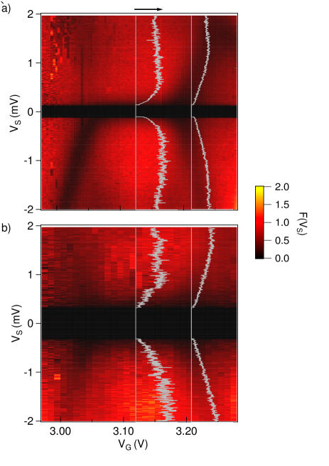
Figure 3: $F(V_{S})=[dS_{I}/dV_{S}]/[e\,dI/dV_{S}(V_{S}-h\nu/e)]$ as a function of the bias voltage $V_{S}$ and the gate voltage $V_{G}$ at $\nu_{1}=29.5$GHz (a) and $\nu_{3}=78$GHz (b). $F(V_{S})$ is arbitrarily fixed to zero for $e|V_{S}|<h\nu$. The gray curves on top of the colorplot correspond to the bias voltage dependence of $F(V_{S})$ at $V_{G}=3.12$V and $V_{G}=3.21$V. The black arrow indicates a value of the $F(V_{S})$ equal to 1. When the conductance is low, $F(V_{S})$ is close to one while it is reduced in the highly conducting regions.

To compute the dashed curves in figure 2, an intrinsic spin decoherence time $\tau_{S}$ induced by the large bias was included and calculated self-consistently in the FRG approach paaske04 (see appendix). The decoherence of the Kondo effect induced by a large dc voltage bias is a well-known feature which has indeed been measured francesci02 ; leturcq05 , and has been predicted to lead to a strong reduction of the Kondo resonance due to inelastic processes paaske04 ; monreal05 ; roermund10 . Since the singularity in the noise at $h\nu\approx eV_{S}$ is associated with the transitions between the two Kondo resonances pinned at the Fermi levels of the contacts, this singularity is also affected by decoherence.

However, as shown in figure 2, the computed intrinsic decoherence time is insufficient to explain the experimentally observed suppression of the peak in $dS_{I}/dV_{S}$. Therefore, we incorporated a voltage-dependent spin relaxation rate in our calculations, $\tau_{S}^{-1}(V_{S})$, which includes external decoherence. The consistency of this approach can be checked against the experiments: a single choice of $\tau_{S}^{-1}(V_{S})$ must simultaneously reproduce the voltage dependence of the differential conductance through the dot $dI/dV_{S}(V_{S})$, and those of the $\nu_{1}=29.5$ GHz and $\nu_{1}=78$ GHz noise spectra, $dS_{I}/dV_{S}(V_{S})$. Furthermore, $\tau_{S}^{-1}$ should be suppressed for $V_{S}<T_{K}^{\rm RG}$. We found that a bias-dependent decoherence rate of the form $h/\tau_{S}\approx\alpha\;k_{B}T^{\rm RG}_{K}{\rm atan}(\beta eV_{S}/k_{B}T^{\rm RG}_{K})$ (similar in shape to the calculated intrinsic spin relaxation rates), with $\alpha=14$ and $\beta=0.15$ satisfied all criteria above. The continuous lines in figure 2 show the $dS_{I}/dV_{S}$ curves computed with this form of $h/\tau_{S}$, and fit fairly well the experimental data for both resonator frequencies. As a final consistency check, we also computed the differential conductance through the dot (taking into account the above form of $\tau_{S}^{-1}$) and compared it to the measured $dI/dV_{S}$ curves. A very good agreement is found without any other adjustable parameter in the voltage-range $V>0.1mV$, where the FRG approach is appropriate (Inset of figure 2b).

From the theoretical fits we infer that the experimentally observed noise spectra and differential conductance can be understood in terms of a decoherence rate, which is about a factor of $2$ larger than the theoretically computed intrinsic rate (see appendix). One possibility for this discrepancy is that the experimentally observed decoherence is intrinsic, and FRG - which is a perturbative approach - underestimates the spin relaxation rate in this regime (which is indeed almost out of the range of perturbation theory). Another possibility is that the experimental set-up leads to additional decoherence.

The experiment also allows to draw a complete map of the noise in the region of the Kondo ridge. We define $F(V_{S})=[dS_{I}/dV_{S}(V_{S})]/[e\,dI/dV_{S}(V_{S}-h\nu/e)]$, i.e. the ratio of the derivative of the noise to the differential conductance shifted in voltage by an amount corresponding to the measured frequency. For both linear and non linear systems with energy independent transmission at low temperature this quantity is equal to the Fano factor blanter00 . We have plotted $F(V_{S})$ for $\nu_{1}=29.5$GHz (figure 3a) and $\nu_{3}=78$GHz (figure 3b). For $|eV_{S}|<h\nu$, where the emission noise is zero, $F(V_{S})$ is arbitrarily fixed to zero. For both frequencies the noise is found to be sub-poissonian, with $F(V_{S})$ close to one in the poorly conducting regions and a strong decrease of $F(V_{S})$ along the conducting regions. This is qualitatively consistent with the reduction of the Fano factor for a conducting channels of transmission close to one. This result has to be contrasted with back scattering noise measurements in the Kondo regime at low frequency and low bias voltage where the Fano factor was found to be higher than one zarchin08 ; yamauchi11 .

In conclusion we have measured the high frequency current fluctuations of a carbon nanotube quantum dot in the Kondo regime by coupling it to a quantum detector via a superconducting resonant circuit. We find that the noise exhibits strong resonances when the voltage bias is of the order of the measurement frequency in good agreement with theory provided that an additional decoherence rate is included which prevents the full formation of the out of equilibrium Kondo resonances. Our experiment constitutes a new original tool for the investigation of the non-equilibrium dynamics of many-body phenomena in nanodevices.

We thank M. Aprili, S. Guéron, M. Ferrier, M. Monteverde and J. Gabelli for fruitful discussions. This work has benefited from financial support of ANR under Contract DOCFLUC (ANR-09-BLAN-0199-01) and C Nano Ile de France (project HYNANO), the EU-NKTH GEOMDISS project, OTKA research Grants No. K73361 and No. CNK80991 and the French-Romanian grant DYMESYS (ANR 2011-IS04-001-01 and contract PN-II-ID-JRP-2011-1).

Appendix : Relation between $T_{K}$ and $T_{K}^{RG}$

To perform the theoretical calculations, one first needs to find the Kondo temperature. However, the Kondo temperature is defined only up to a prefactor, and its value also depends slightly on the physical quantity from which it is defined. Our experimental Kondo temperature, $T_{K}$, is defined as $T_{K}=e\;\Delta V_{S}/k_{B}$, with $\Delta V_{S}$ the half-width at half maximum of the measured $G(V_{S})=dI/dV_{S}$ curves. In the FRG calculations, on the other hand, it is defined as a scale (frequency), $k_{B}T_{K}^{\rm RG}\equiv\hbar\omega_{K}^{\rm RG}$, where the so-called leading logarithmic calculations yield a divergent interaction vertex at $T=0$ temperature. It can, however, also be defined as the temperature, $T_{K}^{\rm T-dep}$, at which the linear conductance drops to half of its $T=0$ temperature value. The ratios of all these Kondo temperatures are just universal numbers (apart from a possible but presumably small dependence of $\Delta V_{S}$ on the anisotropy, $A$).

To determine the ratio of $T_{K}^{\rm T-dep}$ and $k_{B}T_{K}^{\rm RG}$, we performed numerical renormalization group calculations BudapestCode : We computed the full $G(T)$ curve, extracted from it the width $T_{K}^{\rm T-dep}$, and for the same parameters, we also computed $T_{K}^{\rm RG}=\hbar\omega_{K}^{\rm RG}/k_{B}$ from the high-frequency tail of the so-called composite fermions’ spectral function, scaling as $\approx C/\ln^{2}(\omega/\omega_{K}^{\rm RG})$ at large frequencies. In this way, we obtained a ratio

$$T_{K}^{\rm RG}/T_{K}^{\rm T-dep}\approx\;0.3.$$

The ratio $T^{\rm T\;dep}_{K}/T_{K}$ was then determined from experimental data Kouwenhoven , giving

$$T_{K}^{\rm T-dep}/T_{K}\approx 1.2\;.$$

The previous equations yield the ratio, $T_{K}^{\rm RG}/T_{K}\approx 0.36$, used in our calculations and quoted in the main text.

Appendix : Summary of the functional renormalization group approach

In this work we used the functional renormalization group approach developed in Ref. moca11 , an extension of the formalism of Ref. rosch . In this approach, formulated at the level of non-equilibrium action, a short time cut-off $a$ is introduced, and increased in course of the renormalization group (RG) procedure to eliminate the high-energy degrees of freedom. This procedure yields a retarded interaction ($j_{\alpha\beta}\to g_{\alpha\beta}(t-t^{\prime},a)$), whose cut-off dependence is described by the differential equation,

$$\frac{\rm d{\bf g}(\omega,a)}{{\rm d}\ln a}={\bf g}(\omega,a)\;{\bf q}(\omega,a)\;{\bf g}(\omega,a)\;.$$ (5)

Here we introduced the matrix notation, $g_{\alpha\beta}(\omega,a)\to{\bf g}(\omega,a)$ for the Fourier transform of the retarded interaction, and the matrix ${\bf q}(\omega,a)$ denotes a cut-off function. In our calculations we have not approximated this latter with $\Theta$-functions, as in Ref. moca11 , but used a function corresponding to the real time propagators of Ref. moca11 , also incorporating the effect of an exponential decay rate $\Gamma=1/\tau_{S}$.

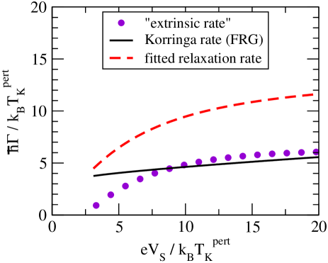
Figure 4: Voltage dependence of the fitted and intrinsic relaxation rates, and their difference, termed as extrinsic spin relaxation rate in the voltage range, $V_{S}\geq 0.1\;{\rm mV}$. The intrinsic rate was calculated by FRG, while the form and overall magnitude of the extrinsic rate were inferred from the differential conductance data.

The voltage-dependent decay rate $\Gamma(V_{S})$ has an intrinsic part, $\Gamma_{\rm intr}(V_{S})$, as well as an external contribution, $\Gamma_{\rm ext}(V_{S})$. The former contribution can be identified as the Korringa spin relaxation rate, and can be expressed as

$$\Gamma_{\rm intr} = \pi\sum_{\alpha,\beta=L,R}\int{\rm d}\omega\,g_{\alpha\beta}(\omega)\;g_{\beta\alpha}(\omega)\;$$ (6)

$$f(\omega-\mu_{\alpha})\;(1-f(\omega-\mu_{\beta}))\;,$$

with $g_{\alpha\beta}(\omega)$ the vertex functions in the limit $a\to\infty$, $\mu_{\alpha}$ the electro-chemical potentials of the leads, and $f$ the Fermi function. The rate $\Gamma_{\rm intr}(V_{S})$, as computed by FRG is shown in Fig. 4. Rather surprisingly, in the cross-over regime, $eV_{S}\sim k_{B}T_{K}^{\rm pert}$, it almost saturates, and only weakly depends on the bias. For a comparison, figure 4 also shows the total fitted relaxation rate, $\Gamma(V_{S})=1/\tau_{S}(V_{S})$ needed to reproduce the differential conductance and noise data. It is not very far from the calculated intrinsic contribution, but it is above the latter, and it apparently includes some extrinsic spin relaxation, too.

In the formalism of Ref. moca11 , the current operator and the current vertex are also renormalized during the RG procedure, and also become non-local. However, the current vertex, $\mathbf{V}$, has a more complicated structure than the interaction vertex, and possesses two non-trivial time arguments, $g_{\alpha\beta}(\omega)\leftrightarrow{V_{\alpha\beta}}(\omega_{1},\omega_{2})$. The evolution of $\mathbf{V}$ under the RG is described by a differential equation similar to equation (5) (see reference moca11 for the details). The noise spectrum, i.e., the Fourier transform of the current-current correlation function can then be expressed as a double integral of this retarded current vertex taken in the limit $a\to\infty$. The emission noise, $S_{e}(\omega)$, e.g., can be expressed as

$$S_{e}(\omega)=\frac{e^{2}}{2}\;S(S+1) \int\frac{{\rm d}\tilde{\omega}}{2\pi}\;{\rm Tr}\{{\bf V}(\tilde{\omega}_{+},\tilde{\omega}_{-}){\bf G}^{>}(\tilde{\omega}_{-})$$ (7)

$${\bf V}(\tilde{\omega}_{-},\tilde{\omega}_{+}){\bf G}^{<}(\tilde{\omega}_{+})\}\;,$$

with $\tilde{\omega}_{\pm}=\tilde{\omega}\pm\frac{\omega}{2}$ and $S=1/2$. Here the trace refers to the labels $\alpha,\beta=L/R$, and the bigger and lesser Green’s functions are given as $G_{\alpha\beta}^{>/<}(\omega)=\pm i\;2\pi\;\delta_{\alpha\beta}\;f(\pm(\omega-\mu_{\alpha}))$.

References

- (1) D. Goldhaber-Gordon et al., Nature 391, 156-159 (1998).
- (2) S.M. Cronenwett, T.H. Oosterkamp and L.P. Kouwenhoven, Science 281, 540-544 (1998).
- (3) J. Nygard, D.H. Cobden and P.E. Lindelof, Nature 408, 342 346 (2000).
- (4) Y. Meir and A. Golub, Phys. Rev. Lett. 88, 116802 (2002).
- (5) E. Sela, Y. Oreg, F. von Oppen and J. Koch, Phys. Rev. Lett. 97, 086601(2006).
- (6) A. Golub, Phys. Rev. B 73, 233310 (2006).
- (7) A.O. Gogolin and A. Komnik, Phys. Rev. Lett. 97, 016602 (2006).
- (8) C. Mora, X. Leyronas and N. Regnault, Phys. Rev. Lett. 100, 036604 (2008).
- (9) T. Delattre et al, Nature Phys. 5, 208 (2009).
- (10) O. Zarchin,M. Zaffalon, M. Heiblum, D. Mahalu, and V. Umansky, Phys. Rev. B 77, 241303(R) (2008).
- (11) Y. Yamauchi et al., Phys. Rev. Lett. 106, 176601 (2011).
- (12) P. Nordlander, M. Pustilnik, Y. Meir, N.S. Wingreen and D.C. Langreth, Phys. Rev. Lett. 83, 808-811 (1999).
- (13) J. Basset, H. Bouchiat and R. Deblock, Phys. Rev. Lett. 105, 166801 (2010).
- (14) A.M. Tsvelick and P.B. Wiegmann, Advances in Physics 32, 453 (1983).
- (15) N.E. Bickers, Rev. Mod. Phys. 59, 845-939 (1987).
- (16) T. Holst, D. Esteve, C. Urbina, and M.H. Devoret, Phys. Rev. Lett. 73, 3455-3458 (1994).
- (17) G. Ingold, and Y.V. Nazarov, Single-Charge Tunneling, edited by Grabert,H. and Devoret, M.H. (Plenum, New-York, 1992).
- (18) A. Barone, and G. Paterno,Physics and Applications of the Josephson effect (Wiley-Interscience, New-York, 1982).
- (19) M. Sindel, W. Hofstetter, J. von Delft, and M. Kindermann, Phys. Rev. Lett. 94, 196602 (2005).
- (20) A. Schiller and S. Hershfield, Phys. Rev. B 58, 14978-15010 (1998).
- (21) T. Korb, F. Reininghaus, H. Schoeller, and J. König, Phys. Rev. B 76, 165316 (2007).
- (22) C.P. Moca, P. Simon, C.H. Chung,and G. Zarand, Phys. Rev. B 83, 201303(R) (2011).
- (23) J. Paaske, A. Rosch, J. Kroha, and P. Woelfle, Phys. Rev. B 70, 155301 (2004).
- (24) S. De Franceschi, et al, Phys. Rev. Lett. 89, 156801(2002).
- (25) R. Leturcq, et al, Phys. Rev. Lett. 95, 126603 (2005).
- (26) R.C. Monreal, and F. Flores, Phys. Rev. B 72, 195105 (2005).
- (27) R. van Roermund, S. Shiau, and M. Lavagna, Phys. Rev. B 81, 165115 (2010).
- (28) Y.M. Blanter, and M. Büttiker, Phys. Rep. 336, 1 (2000).
- (29) Yu.A. Kasumov, et al, Appl. Phys. A 88, 687 691 (2007).
- (30) We used the open access Budapest DM-NRG code, http://neumann.phy.bme.hu/~dmnrg/.
- (31) For our calculations we used the Budapest NRG code (http://neumann.phy.bme.hu/~dmnrg/), developed by Legeza, O., Moca, C.P., Toth, A. I., Weymann, I., and Zarand, G.; For technical details see also A.I. Toth, C.P. Moca, O. Legeza, and G. Zarand, Phys. Rev. B 78, 245109 (2008).
- (32) W.G. van der Wiel et al., Science 289, 2105 (2000).
- (33) A. Rosch, J. Kroha, and P. Wölfle,, Phys. Rev. Lett. 87, 156802 (2001)