Super-Eccentric Migrating Jupiters

Abstract

An important class of formation theories for hot Jupiters involves the excitation of extreme orbital eccentricity ($e=0.99$ or even larger) followed by tidal dissipation at periastron passage that eventually circularizes the planetary orbit at a period less than 10 days. In a steady state, this mechanism requires the existence of a significant population of super-eccentric ($e>0.9$) migrating Jupiters with long orbital periods and periastron distances of only a few stellar radii. For these super-eccentric planets, the periastron is fixed due to conservation of orbital angular momentum and the energy dissipated per orbit is constant, implying that the rate of change in semi-major axis $a$ is $\dot{a}\propto a^{1/2}$ and consequently the number distribution satisfies $d{\mathcal{N}}/d\log a\propto a^{1/2}$. If this formation process produces most hot Jupiters, Kepler should detect several super-eccentric migrating progenitors of hot Jupiters, allowing for a test of high-eccentricity migration scenarios.

1. Introduction

The origin of gas-giant planets with orbital periods of only a few days – the hot Jupiters – is not understood. One hypothesis involves the following sequence of events: (i) the planets form at a few AU from their host stars, in approximately circular orbits; (ii) some mechanism excites their orbits to extreme eccentricities ($1-e\lesssim 0.01$); (iii) tidal dissipation during successive periastron passages removes enough orbital energy so that the planet migrates a factor of $\sim 100$ in semi-major axis, finally settling into a circular orbit close to the host star. Possible excitation mechanisms include Kozai–Lidov (KL) oscillations (Wu & Murray 2003; Fabrycky & Tremaine 2007), planet-planet scattering (Rasio & Ford 1996; Nagasawa et al. 2008), resonant capture during migration in multi-planet systems (Yu & Tremaine 2001), and weak resonant orbital interactions (called “secular chaos” by Wu & Lithwick 2011). We shall refer to these as high-eccentricity migration (HEM) scenarios; they are of particular interest because they naturally predict frequent misalignment of the stellar spin and planetary orbit, consistent with recent observations of the Rossiter-McLaughlin effect (Winn et al. 2010).

Most hot Jupiters have relatively small eccentricities: 60% of the known planets with orbital period $P<10\,\hbox{d}$ and $M\sin i>0.25M_{J}$ (Jupiter masses) have eccentricities consistent with zero, and 90% have eccentricity $e<0.1$. If the hot Jupiters are formed through the HEM process, this result implies that the timescale for the decay of the eccentricity from near unity to near zero is short compared to the age of the Galaxy. Since the star-formation rate is approximately constant over the age of the Galaxy, the distribution of migrating Jupiters with moderate or high eccentricity should therefore be in an approximate steady state. Moreover, for these eccentricities the energy dissipation per orbit is independent of eccentricity, since the dissipation occurs only near periastron and in this region all moderate and high-eccentricity orbits look like parabolae. Therefore, we can predict the eccentricity and semi-major axis distribution in HEM independent of the details of the dissipation process. We do this in §2 and find that HEM requires the presence of a large population of Jupiters with eccentricity $e\gtrsim 0.9$, which we call “super-eccentric” Jupiters. Quantitative predictions and a strategy for detection using Kepler targets are in §3. A brief summary is given in §4.

2. Steady-State Distribution of Migrating Jupiters

2.1. Basic assumptions

Migration from large to small semi-major axis requires that energy is removed from the orbit. In HEM, tidal friction is responsible for converting orbital energy into heat which is then radiated away from the system. In most cases, tidal friction in the planet removes energy much faster than tidal friction in the star. Since the planet’s spin angular momentum is negligible compared to its orbital angular momentum, the orbital angular momentum per unit mass $J$ is conserved during HEM (however, see discussion in §2.4), i.e.,

$$J^{2}=G\left(M_{\star}+M_{p}\right)a\left(1-e^{2}\right)={\rm cst.}$$ (1)

where $a$, $M_{p}$, $M_{\star}$ and $G$ are the semi-major axis, planet mass, host star mass and gravitational constant, respectively. Thus

$$a\,\left(1-e^{2}\right)=q(1+e)\equiv a_{{}_{\rm F}}={\rm cst.}$$ (2)

where $q$ is the periastron distance and $a_{{}_{\rm F}}$ is the final semi-major axis that the planet reaches when the eccentricity has decayed to zero.

Let $X=e$ or $a$, and let ${\mathcal{N}}_{J}(X)\,dJ$ be the number of migrating planets with eccentricity or semi-major axis less than $X$ and angular momentum in the interval $(J,J+dJ)$. We assume that all planets with eccentricity greater than some reference value $e_{\rm ref}$ are still migrating, and set ${\mathcal{N}}_{J}(e_{\rm ref})=0$. We have argued that the distribution of migrating planets is in steady state and that orbital angular momentum is conserved during migration. Then the continuity equation requires

$$\dot{X}\,\frac{d{\mathcal{N}}_{J}}{dX}={\mathcal{S}}_{J}$$ (3)

where ${\mathcal{S}}_{J}dJ$ is the current of migrating planets with angular momentum in the interval $(J,J+dJ)$. This current is determined by the properties of the source of highly eccentric long-period gas giants, which is assumed to be far ($a\gg 1\,\hbox{AU}$) from the region of phase space under consideration.

2.2. Orbital evolution: approximate treatment at high eccentricity

We now describe an approximate analytic treatment of the orbital evolution and steady-state distribution at high eccentricity. For high eccentricity the shape of the orbit near periastron and the energy loss per periastron passage $\Delta E$ are both independent of $e$. Thus the orbit-averaged energy loss rate is

$$\dot{E}=\frac{\Delta E}{P}\propto\frac{1}{P}\propto a^{-3/2}$$ (4)

where $P$ is the orbital period. Since $E\propto 1/a$

$$\Big{|}\frac{da}{dt}\Big{|}\propto a^{1/2}.$$ (5)

In the region of $(e,a)$ space that contains a steady-state distribution of migrating planets on high-eccentricity orbits ($q=a(1-e)\lesssim 10R_{\odot}$ for Sun-like host stars) the number of migrating Jupiters per unit semi-major axis is found with the help of equation (3),

$$\frac{d{\mathcal{N}}_{J}}{da}=\frac{{\rm cst.}}{\dot{a}}\propto a^{-1/2}\quad\mbox{or}\quad\frac{d{\mathcal{N}}_{J}}{d\log a}\propto a^{1/2}.$$ (6)

2.3. Orbital evolution: exact treatment

In order to study orbital evolution at small or moderate eccentricity, some understanding of tidal dissipation is required. Unfortunately there is no robust theory of tidal dissipation in gas-giant planets, due both to the sparseness of observational calibration (only Jupiter and Saturn) and to theoretical difficulties in studying such weak dissipation (e.g., tidal $Q\sim 10^{5}$ for the Jupiter-Io system).

For illustration, we shall use the phenomenological approach of Hut (1981), which follows Darwin in assuming that the tides lag their equilibrium value by a constant time $\tau$. By assuming pseudo-synchronous rotation (Hut’s eq. 45) we find that the orbital evolution for a single planet is described by

$$\frac{de}{d\tilde{t}}=-\frac{1}{2}e(1-e^{2})^{3/2}g(e)$$ (7)

which is equivalent to

$$\frac{d\tilde{a}}{d\tilde{t}}= -\,\tilde{a}^{1/2}\,e^{2}g\left(e\right)$$ (8)

where $\tilde{a}\equiv a/a_{{}_{\rm F}}=(1-e^{2})^{-1}$ and $\tilde{t}\equiv t/t_{D}$. Here ${t_{D}=M_{p}\,a^{8}_{{}_{\rm F}}/\left(9\,k\,G\,M^{2}_{\star}\,R^{5}_{p}\,\tau\,\right)}$ is a dissipation time, $k\simeq 0.5$ is the planet’s Love number, and $R_{p}$ is its radius. This result assumes $M_{p}\ll M_{\star}$. The function $g(e)$ is given by

$$g(e)= \frac{7+\frac{45}{2}e^{2}+56e^{4}+\frac{685}{32}e^{6}+\frac{255}{64}e^{8}+\frac{25}{256}e^{10}}{3(1+3e^{2}+\frac{3}{8}e^{4})}$$

$$\simeq \,2.33+6.12e^{3}$$ (9)

where the approximation in the final equation is accurate to better than 0.5% for all eccentricities between 0 and 1.

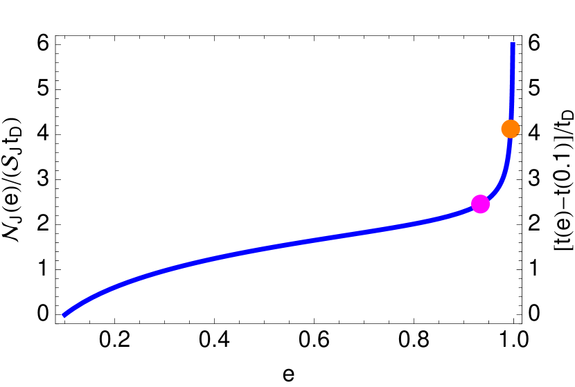
Figure 1.— Cumulative distribution of migrating planets ${\mathcal{N}}_{J}(e)$ with eccentricity $e>e_{\rm ref}=0.1$, from equation (11). The planets migrate along a track of constant orbital angular momentum $J$. The vertical axis also represents the time required for the eccentricity to decay to $e_{\rm ref}$. The magenta dot represents the current position of HD 80606b ($e=0.94$, $a=0.45$ AU) and the orange dot represents a hypothetical planet with semi-major axis $a=5$ AU flowing along the same angular-momentum track as HD 80606b. The number of objects in the range $e=0.94-0.995$ is comparable to the number of objects in the range $e=0.2-0.94$. The plot is shown in normalized units so the curves are independent of $J$.

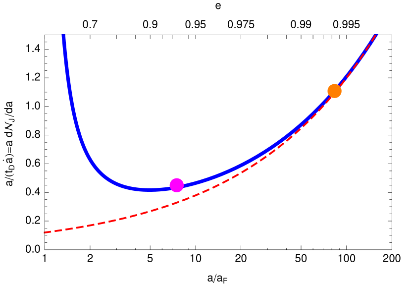
Figure 2.— The blue curve shows the distribution $d{\mathcal{N}}_{J}/d\log a$ of migrating Jupiters per unit interval in angular momentum $J$ from equation (10) and the dashed red curve shows the high-eccentricity approximation $d{\mathcal{N}}/d\log a\propto a^{1/2}$ (eq. 6). The high-eccentricity approximation is accurate to $\sim 20\%$ for $a/a_{{}_{\rm F}}\gtrsim 10$ or $e\gtrsim 0.95$. The magenta and orange points have the same meaning as in Figure 1. The plot is shown in normalized units so the curves are independent of $J$.

Equation (3) then implies that the number of planets per unit interval in angular momentum is given by

$$\frac{d{\mathcal{N}}_{J}(e)}{de}=\frac{{\mathcal{S}}_{J}}{|de/dt|},$$ (10)

and

$${\mathcal{N}}_{J}(e)=\int_{e_{\rm ref}}^{e}d{\mathcal{N}}_{J}(e)={\mathcal{S}}_{J}\left[t(e)-t(e_{\rm ref})\right]$$ (11)

where $t(e)$ is the time required to migrate from some initial eccentricity near unity to $e$. The cumulative distribution ${\mathcal{N}}_{J}(e)$ for a single track in $J$, as determined from equations (7) and (11), is shown in Figure 1.

Figure 2 displays the expected number of migrating Jupiters per unit $\log a$, as obtained from equation (8), as well as the high-eccentricity approximation (6). For a fixed interval in orbital angular momentum, the number of migrating Jupiters is an increasing function of $\log a$ above $e\simeq 0.9$.

2.4. The approximation of constant orbital angular momentum

In HEM scenarios, gas giants are assumed to be born on nearly circular orbits and then acquire a large eccentricity after exchanging their angular momentum with other planets or distant stellar companions, through close encounters in the former case or Kozai–Lidov (KL) oscillations in the latter. Therefore, orbital angular momentum is not a constant during the process of eccentricity excitation. Our analysis assumes that eccentricity excitation takes place at large semi-major axes (say, $a\gtrsim 5$–10 AU) and focuses on the region of $(a,e)$ space where substantial orbital decay has already occurred but the eccentricity is still moderate to large (say $a\lesssim 1$ AU and $e>0.2$). It is not clear whether or not the approximation that migration takes place at constant angular momentum is accurate for all semi-major axes $a\lesssim 1$ AU. In what follows, we assess the validity of the constant $J$ approximation of §§2.2 and 2.3 in the presence of KL oscillations, which are the most likely cause of changes in the orbital angular momentum of the migrating planet.

We performed many numerical integrations of the orbit-averaged restricted three body problem, including the effects of general relativity, tidal dissipation and tidal precession. Each simulation was initialized with a Jupiter-mass planet orbiting about a solar-mass star, placed in a nearly circular orbit with semi-major axis $a\simeq 3-5$ AU. The system also contained a solar-mass companion star, placed at distances of $30-1000$ AU with inclination of $85^{\circ}\leq i\leq 90^{\circ}$ relative to the planetary orbit. Only the quadrupole term of the companion’s potential was considered.

Typically, KL oscillations commenced at the start of the integration, with large amplitude variations in orbital angular momentum $J$. Due to the strong dependence of tidal dissipation on periastron distance $q$, dissipation takes place almost entirely in the vicinity of $J_{\rm min}$, the minimum orbital angular momentum during a KL oscillation. As a result, the value of $J_{\rm min}$ remains roughly fixed during migration. Precession due to general relativity acts to decrease the amplitude of the oscillation in $J$ (e.g., Blaes et al. 2002; Wu & Murray 2003; Fabrycky & Tremaine 2007). Once the oscillation amplitude in $J$ is sufficiently small ($<10\%$ in $J$), such that the dissipation rate does not change considerably during each cycle, the mean value of $J$ remains constant and equal to the final orbital angular momentum $J_{\rm F}$. Therefore, the distribution of planets from then on can be computed by assuming a constant $J=J_{\rm F}$. At this stage of migration, KL oscillations are considered to be ”quenched.” Quantitatively, KL oscillations are quenched at a semi-major axis $a_{\rm Q}$ given by

$$a_{\rm Q}\approx 1.8{\rm AU}\,\left(\frac{a_{\rm F}}{0.05{\rm AU}}\right)^{-1/7}\left(\frac{\sin^{2}i_{\rm min}}{0.4}\right)^{-2/7}\left(\frac{M_{\star}}{M_{\odot}}\right)^{4/7}$$

$$\times\left(\frac{M_{\rm per}}{M_{\odot}}\right)^{-2/7}\left(\frac{a_{\rm per}}{1000\,{\rm AU}}\right)^{6/7}\left(\frac{1-e_{\rm per}^{2}}{1-0.5^{2}}\right)^{3/7}$$ (12)

where $a_{\rm per}$ and $e_{\rm per}$ are the semi-major axis and eccentricity of the perturber and $i_{\rm min}$ is the mutual inclination at the phase of the KL oscillation when $J=J_{\rm min}$, while $M_{\rm per}$ is the perturber mass. For larger perturber mass or smaller semi-major axis, KL oscillations are quenched closer to the host star. In particular, nearby giant planets quench the oscillations at smaller radii than distant companion stars; for example, a Jupiter-mass perturber at $10$ AU has $a_{Q}\approx 0.2$ AU. The major difference between our various integrations of KL oscillations with tidal dissipation was the value of $a_{Q}$, due primarily to variations in the distance of the perturber.

During each integration we tracked the time that the planet spent in a bin of width $\Delta J$ centered on the final angular momentum $J_{\rm F}$. We used this information to construct the eccentricity and semi-major axis distributions that would be present in this angular momentum bin in a steady-state population of planets following this migration path. We found that even in the presence of KL oscillations the constant $J$ approximation described in §§2.2 and 2.3 reproduced the distribution of planets to within a factor of two or better, so long as $\Delta J$ was not more than about 20% of $J_{\rm F}$. That is, we found that the steady-state formulas derived in §2.3 by assuming constant $J$ were still approximately valid, even though the orbital angular momentum experiences large amplitude oscillations (see example of HD 80606b in §2.5).

This surprising agreement results from the fact that tidal dissipation, and thus migration, occurs mostly when $J\simeq J_{\rm min}$, the minimum value of the angular momentum during a Kozai–Lidov cycle. As long as $J_{\rm min}$ is close to $J_{\rm F}$, the final value of orbital angular momentum after quenching, then all of the migration takes place within the bin of width $\Delta J$. The time that the planets spend on Kozai–Lidov cycles outside the bin is irrelevant, since they do not migrate there.

2.5. An example

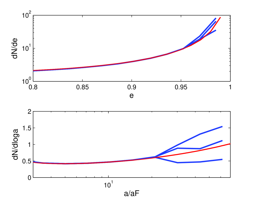
Figure 3.— Comparison of the analytic theory (red) of §2.3 with the migration of HD 80606b, as depicted in Figure 1 of Fabrycky & Tremaine (2007). The blue lines show the density in eccentricity and log semi-major axis of a steady-state ensemble of planets that all follow the same trajectory as HD 80606b. The planets only contribute to the density when their angular momentum is small, in particular when $a\,(1-e^{2})\leq 0.14,0.11$ and $0.08$ AU. The normalization is chosen so that all the curves match at $a/a_{\rm F}=5$. Despite the presence of KL oscillations for $a/a_{{}_{\rm F}}\gtrsim 30$, the density is approximated by the analytic expressions derived in §2.3 to within a factor of two for all values of $(e,a)$.

Consider the migration of the gas-giant planet HD 80606b, which currently has $a=0.45$ AU and $e=0.93$, corresponding to $a_{{}_{\rm F}}=a(1-e^{2})=0.06$ AU. The migration track has been modeled by Wu & Murray (2003) and Fabrycky & Tremaine (2007), who start with an initially nearly circular orbit with $a=5$ AU, similar to Jupiter. KL oscillations are excited by a distant companion star HD 80607. For the first Gyr of the evolution the eccentricity oscillates between $e_{\rm max}=0.993$ and $e_{\rm min}=0.04$–$0.25$. The amplitude of the KL oscillations then gradually decays; the oscillations are quenched by 2.8 Gyr, when the eccentricity is 0.97 and the semi-major axis is 2 AU – in agreement with equation (12) – and thereafter the eccentricity and semi-major axis decay at constant angular momentum, reaching zero eccentricity after 4 Gyr at a semi-major axis $a_{\rm F}=0.071$ AU.

In Figures 1 and 2 the magenta and orange points represent the current position of HD 80606b and its hypothetical Jupiter-like “progenitor,” respectively.

Figure 3 shows in blue the density of planets in eccentricity and semi-major axis that would result from a steady-state ensemble of migrating planets with the same trajectory as HD 80606b. Three plots are shown, for angular-momentum cutoffs $J_{c}^{2}=G(M_{\star}+M_{p})a_{c}$ with $a_{c}=0.14,0.11$, and 0.08 AU (top to bottom). For comparison, the red lines show the analytical predictions of §2.3. In the latter stages of migration, after the KL oscillations have been damped, the density matches the analytical estimate extremely well—this is not surprising since the assumption of evolution at constant angular momentum is satisfied to high accuracy. At larger eccentricities and semi-major axes, when KL oscillations are present, the blue curves are displaced from extrapolation of these theoretical predictions by up to a factor of two or so, but their shapes remain similar as expected from the arguments of the preceding subsection.

All three of Figures 1, 2 and 3 show that in a steady state, an unbiased sample of exoplanets containing one HD 80606b should contain more than one migrating planet with a similar periastron distance and even larger semi-major axis and eccentricity.

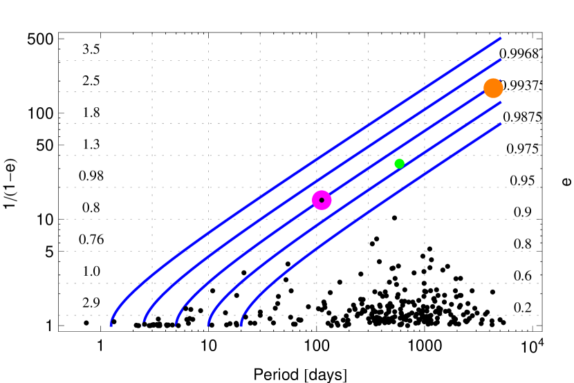
Figure 4.— In solid blue are lines of constant angular momentum $J$ that correspond to $P_{{}_{\rm F}}=P(1-e^{2})^{3/2}=1.25,\,2.5,\,5.0,\,10.0,\,{\rm and}\,20.0$ days. Horizontal dotted lines are fixed values of $1/1-e$, separated by factors of two. The corresponding values of $e$ (0.2, 0.6, etc.,) are on the right hand side of the figure. The relative number of planets expected in each interval along a track in constant $J$ is given by the numbers on the left (2.9, 1.0, etc.,). Tidal dissipation drives the planets to flow from the upper right corner to the lower left corner, along the lines of constant $J$. Black dots are current RV observations with $M\sin i>0.25$ taken from exoplanet.org with the exception of HD 20782b (green dot) for which the updated $e=0.97$ (O’Toole et al. 2009) is used. The magenta dot highlights the current position of HD 80606b and the orange dot represents a hypothetical planet at $5$ AU flowing along the same track in $J$ as HD 80606b.

3. Observations, Predictions, and Discussion

3.1. Current observations

We compile a list of all known exoplanets with $M\sin i>0.25M_{J}$, of which the radial-velocity planets are displayed in Figure 4. The planetary parameters are taken from exoplanets.org with the exception of HD 20782b, the green dot, whose eccentricity was recently revised to $e=0.97$ (O’Toole et al. 2009). For each planet we compute $P_{{}_{\rm F}}=P(1-e^{2})^{3/2}$, the final orbital period that a planet would reach if its eccentricity decayed to zero at constant angular momentum. For reference a planet with Jupiter’s orbital period and $P_{{}_{\rm F}}=10\,\mbox{d}$ would have $e=0.991$.

The blue lines in Figure 4 are lines of constant orbital angular momentum, along which planets flow from long to short orbital periods. The relative number of planets expected in each interval along a track in constant $J$ is given by the numbers on the left (2.9, 1.0, etc.,). If for example, one gas giant planet is found migrating in the $P_{\rm F}$ = 5-10 d bin within an eccentricity range $0.9<e<0.95$ (such as HD 80606b), then there should be $\gtrsim 1$ planet migrating in this 5-10 d bin within an eccentricity range $0.95<e<0.975$ as well.

Among the known gas-giant exoplanets there is a significant excess population having eccentricity consistent with zero and $P=P_{{}_{\rm F}}<10\,\hbox{d}$, corresponding to $a<0.09\,\mbox{AU}$ for a solar-mass host star. In the HEM scenario, these are planets that were formed at several AU, excited to high eccentricity, migrated due to tidal friction, and have now completed the migration process. There is no such excess for larger periods; in HEM models this implies that tidal dissipation is unimportant for planets with $P_{{}_{\rm F}}>10\,\mbox{d}$ and we discard these from our sample.

From the remaining sample we calculate the number of “moderately eccentric” planets, which we define to be those with $0.2<e<0.6$, and the number of “super-eccentric” planets ($e>0.9$). The first two lines of Table 1 summarize the number of gas-giant planets with moderate eccentricity, as detected by radial-velocity (RV) surveys and transit photometry with spectroscopic follow-up (“Transit+RV”). Both the RV and Transit+RV categories yield a fraction of moderate-eccentricity planets that is roughly $1/2$ in the 5–10 d bin and much smaller, $\lesssim 1/15$, in the 3–5 d bin. The sharp decline for smaller values of $P_{{}_{\rm F}}$ is consistent with the expectation that tidal dissipation is stronger for orbits with smaller periastron, so that in a steady state the fraction of planets in the migration pipeline is smaller.

In HEM models both the moderately eccentric and super-eccentric planets are in steady-state migration and therefore the population ratio in these groups can be calculated using the models of §2.3. Thus we can predict the number of super-eccentric planets that should have been found in RV surveys; this prediction is shown in boldface in the third line along with the number of super-eccentric planets actually found so far in these surveys. Furthermore, the fractions of moderately eccentric RV and Transit+RV planets can be used with our models to predict the number of super-eccentric planets in the Kepler sample (Borucki et al. 2011); this prediction is shown in boldface in the last line of the Table.

Before discussing these predictions we address selection effects. RV surveys may be biased against the detection of super-eccentric planets for at least two distinct reasons. First, sparse observations of high-eccentricity orbits are likely to miss the strong reflex velocity signal near periastron, leading to non-detection of planets that would be detected at the same semi-major axis and smaller eccentricity, or to an underestimate of the eccentricity if the planet is detected (Cumming 2004, O’Toole et al. 2009). This bias only sets in for $e\gtrsim 0.6$ so the fraction of moderately eccentric planets detected in RV surveys is much more reliable than the fraction of super-eccentric planets. Second, we are mostly concerned with avoiding biases against detecting highly eccentric planets at a given angular momentum (i.e., along a given migration track), rather than at a given semi-major axis. Here there is an additional bias, since high-eccentricity orbits have longer periods and hence a periodic signal is harder to detect and characterize in a given time baseline.

Despite these poorly understood selection effects, the predicted and observed numbers of super-eccentric planets in RV surveys as shown in Table 1 are consistent. However, the numbers are too small to test the validity of HEM scenarios.

Table 1Expected number of super-eccentric planets

${P_{{}_{\rm F}}}=P(1-e^{2})^{3/2}$	3–5 days	5–10 days
RV (moderate/total)	0/13	4/9
Transit+RV (moderate/total)	3/46	3/8
RV (super-eccentric, theory/observed)	0 vs. 0	2–3 vs. 2
Kepler (super-eccentric, theory)	2	3– 5

For transit surveys the selection effects can be divided into geometric effects, which depend on the orientation of the observer relative to the star (i.e., whether or not a planet transits the star), and survey effects, which depend on properties of the survey (time baseline, photometric accuracy, etc.). With adequate baseline and signal-to-noise ratio, the most important selection effect is geometrical: the probability that the planet will transit is given by

$${\mathcal{P}}=\left\langle R_{\star}/r\right\rangle_{\phi}=\frac{R_{\star}}{a\,\left(1-e^{2}\right)}=\frac{R_{\star}}{a_{{}_{\rm F}}}\propto\frac{R_{\star}}{J^{2}}.$$ (13)

where $R_{\star}$ and $r$ are the stellar radius and heliocentric distance of the planet during transit and $\langle\rangle_{\phi}$ is an average over the azimuth of the sightline, which is equal to an average over the true anomaly. Therefore, on a migration track of constant angular momentum, the geometric selection effects are independent of eccentricity. That is, a hot Jupiter progenitor with say, $a=1$ AU and $e=0.975$ has the same detection probability as a circularized hot Jupiter with $a=0.05$ and $e=0$. Survey selection effects, in contrast, are biased against high-eccentricity orbits because the period is longer so there are fewer transits in a given period, and because the transits are shorter so the signal/noise ratio is smaller. However, these selection effects can be calculated and corrected for using the methods outlined in Borucki et al. (2011), and should be relatively small since our sample is restricted to giant planets, which are relatively easy to detect.

3.2. Predictions for Kepler

Kepler observations yield the planetary radius $R$ and orbital period $P$. To compare these results to our models we assume that our mass limit, $0.25M_{J}$, corresponds to $R=8R_{\oplus}$ and that the planet population within a range of period is roughly the same as the population within the same range of $P_{{}_{\rm F}}=P(1-e^{2})^{3/2}$ since most planets have small eccentricities. The most recent Kepler catalog (Borucki et al. 2011) contains 30 planets with $R\geq 8R_{\oplus}$ and 3 d$\,\leq P\leq 5\,$d, and 16 in the same radius range with 5 d$\,\leq P\leq 10\,$d.

These can be combined with the results from ground-based surveys (line 2 of Table 1) to predict the number of moderate-eccentricity planets in each period range, and these numbers are combined with the steady-state HEM models in §2.3 to predict the numbers of super-eccentric planets in the Kepler catalog (line 4 of Table 1). These predictions should be underestimates since Kepler will detect planets with longer periods as the mission progresses (the automated pipeline in Borucki et al. 2011 only finds objects with $P<93$ d).

These results imply that Kepler should detect several super-eccentric ($e>0.9$) giant planets ($R>8R_{\oplus}$) with orbital period ¡2 yr. If an extended Kepler mission permits detections of planets with longer periods the predicted number is higher. A significant fraction of these could have $e>0.94$ i.e., more eccentric than HD 80606b, the current confirmed record-holder.

A typical member of this population, with $a_{{}_{\rm F}}=0.1$ AU and $M>0.25M_{J}$, produces a stellar reflex velocity $>50\,\mbox{m s}^{-1}$ near periastron. For objects on highly eccentric orbits with random orientations, most transits occur near periastron, where the reflex velocity is close to the periastron value—quantitatively, over half of all transits occur when the reflex velocity is within 10% of the periastron velocity. Thus relatively few low-exposure RV measurements near the transit epoch should be sufficient to detect and measure a large eccentricity. We suggest that all of the Kepler gas-giant planetary candidates with periods above $\gtrsim 20$ d (Borucki et al. 2011 list $34$ objects with $R>8R_{\oplus}$ and periods between 20 d and 93 d) be followed spectroscopically near transit (with one or two additional measurements at other phases to determine the systemic velocity).

4. Summary and Discussion

The main result of this paper is that if hot Jupiters are formed by high-eccentricity migration (HEM), then there must be a steady-state current or flow of gas-giant planets migrating from large to small orbital periods. Since tidal dissipation is required for HEM and is only effective out to distances of a few stellar radii in typical exoplanet systems, the current must consist of planets that either have periastrons of a few stellar radii or undergo Kozai–Lidov oscillations or other dynamical processes that regularly bring their periastrons to these small values. Moreover, because energy loss from tidal dissipation only occurs near periastron, the rate of energy loss on high-eccentricity orbits varies inversely with the orbital period; thus for every migrating planet on a moderate-eccentricity orbit there should be many super-eccentric planets ($e>0.9$). We have computed the expected eccentricity and semi-major axis distribution of the steady-state current of migrating planets using Hut’s (1981) model of tidal dissipation and assuming pseudo-synchronous planetary spin. Our results indicate that several super-eccentric gas-giant planets should be present in the Kepler exoplanet catalog. These can be discovered, if present, by a program of radial-velocity measurements on the Kepler planets with the largest diameters and the longest periods.

The absence of a significant number of super-eccentric migrating Jupiters in this sample would imply either that HEM is not an ingredient of the formation process for most hot Jupiters, or that our migration model is oversimplified. In particular, we assume that migration occurs at constant orbital angular momentum but argue that our results should be approximately correct even in the presence of Kozai–Lidov oscillations or other processes.

The simple HEM model described here, whose central components are the steady-state approximation and the assumption that migration occurs at constant angular momentum, provides a preliminary framework for the exploration of the dynamics of HEM. A thorough exploration of this dynamics should establish whether our simplified model is accurate and enable a definitive observational test of whether hot Jupiters form through HEM.

References

- Blaes et al. (2002) Blaes, O., Lee, M. H., & Socrates, A. 2002, ApJ, 578, 775
- Borucki et al. (2011) Borucki, W. J., et al. 2011, ApJ, 736, 19
- Cumming (2004) Cumming, A. 2004, MNRAS, 354, 1165
- Fabrycky & Tremaine (2007) Fabrycky, D., & Tremaine, S. 2007, ApJ, 669, 1298
- Hut (1981) Hut, P. 1981, A&A, 99, 126
- Nagasawa et al. (2008) Nagasawa, M., Ida, S., & Bessho, T. 2008, ApJ, 678, 498
- O’Toole et al. (2009) O’Toole, S. J., Tinney, C. G., Jones, H. R. A., Butler, R. P., Marcy, G. W., Carter, B., & Bailey, J. 2009, MNRAS, 392, 641
- Rasio & Ford (1996) Rasio, F. A., & Ford, E. B. 1996, Science, 274, 954
- Winn et al. (2010) Winn, J. N., Fabrycky, D., Albrecht, S., & Johnson, J. A. 2010, ApJ, 718, L145
- Wright et al. (2011) Wright, J. T., et al. 2011, PASP, 123, 412
- Wu & Lithwick (2011) Wu, Y., & Lithwick, Y. 2011, ApJ, 735, 109
- Wu & Murray (2003) Wu, Y., & Murray, N. 2003, ApJ, 589, 605
- Yu & Tremaine (2001) Yu, Q., & Tremaine, S. 2001, AJ, 121, 1736