Fermi polarons in two dimensions

Abstract

We theoretically analyze inverse radiofrequency (rf) spectroscopy experiments in two-component Fermi gases. We consider a small number of impurity atoms interacting strongly with a bath of majority atoms. In two-dimensional geometries we find that the main features of the rf spectrum correspond to an attractive polaron and a metastable repulsive polaron. Our results suggest that the attractive polaron has been observed in a recent experiment [Phys. Rev. Lett. 106, 105301 (2011)].

The behavior of a mobile impurity (polaron) interacting strongly with a bath of particles is one of the basic many-body problems studied in condensed matter physics anderson1967 ; mitra1987 ; devreese2009 ; radzihovsky2010 . With the advent of ultracold atomic gases bloch2008 , the Fermi polaron problem in which a single spin-$\downarrow$ atom interacts strongly with a Fermi sea of spin-$\uparrow$ atoms, has become a subject of intensive research chevy2010 . In three dimensions it was found that the polaron state splits into two branches, a low-energy state interacting attractively with the bath of fermions, and the repulsive polaron, which is an excited, metastable state cui2010 ; schmidt2011 ; massignan2011 . In this way the polaron exemplifies a more general paradigm of a many-body system driven into a nonequilibrium state where a small number of high energy excitations interact strongly with the surrounding degrees of freedom schmitt2008 ; freericks2009 . The polaron is the limiting case of a Fermi gas with strong spin imbalance, and the repulsive polaron provides insight into the question whether a quenched, repulsive Fermi gas may undergo a transition to a ferromagnetic state even though it is highly excited jo2009 ; cui2010 ; schmidt2011 ; massignan2011 ; pekker2011 . Similarly, the ground state of the polaron problem has important implications for the phase diagram of a strongly interacting Fermi gas schirotzek2009 ; nascimbene2009 ; punk2009 .

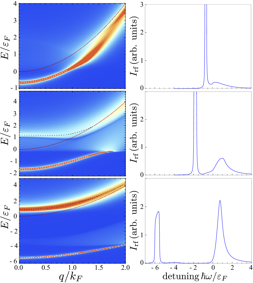
Figure 1: (color online). Left panels: spectral function $\mathcal{A}_{\downarrow}(q,E-\mu_{\downarrow})$ for impurity atoms interacting with a 2D Fermi sea. Red lines indicate the free particle dispersion and white (black) dashed lines mark the dispersion of the attractive (repulsive) polaron. Right panels: corresponding rf spectra illustrating how weight is shifted from the attractive polaron state (peak at negative frequencies) to the new repulsive polaron state at positive frequencies. The two-body bound state energy is (a) $\varepsilon_{B}/\varepsilon_{F}=0.1$, (b) $\varepsilon_{B}/\varepsilon_{F}=1$, (c) $\varepsilon_{B}/\varepsilon_{F}=5$.

It is a key question how many-body properties are affected by reduced dimensionality, and the polaron is a case in point. The combination of optical lattices and Feshbach resonances bloch2008 provides a unique setting to experimentally study strongly interacting low dimensional systems using ultracold atoms froehlich2011 ; dyke2011 . Recent advances in radiofrequency (rf) spectroscopy afford to measure energy spectra schirotzek2009 and give access to excited states as well as full spectral functions using momentum resolved rf stewart2008 ; feld2011 . So far, only the ground state of the two-dimensional polaron problem has been investigated theoretically zoellner2011 ; parish2011 ; klawunn2011 with the focus on a possible polaron to molecule transition. This is similar to the 3D situation where for strong interactions it becomes energetically favorable for the impurity to form a molecular bound state prokofev2008fermi . The structure of high energy excitations and the experimental polaron signatures in rf spectroscopy have remained open questions which we address in this work. We derive the spectral functions of both the molecule and the impurity atom (Fig. 1 left) and find that the impurity state splits into the attractive and the repulsive branch. We compute rf spectra for homogeneous 2D systems (Fig. 1 right) as well as for the experimentally relevant quasi-2D geometries (Fig. 4). Finally, we argue that our calculation provides an alternative explanation of the recent experiment by Fröhlich et al. froehlich2011 in terms of the polaron picture.

A quasi-2D geometry can be realized experimentally using an optical lattice in one direction with associated trapping frequency $\omega_{z}$. In this case, a confinement induced two-body bound state exists for an arbitrarily weak attractive interaction landau1981 ; randeria1989 ; petrov2001 with binding energy $\varepsilon_{B}>0$. The spatial extent of the bound state is related to the 2D scattering length given by $a_{\text{2D}}=\hbar/\sqrt{m\varepsilon_{B}}>0$. In the weak coupling BCS regime of small 3D scattering length $a_{\text{3D}}<0$ bloch2008 these dimers are large and weakly bound ($\varepsilon_{B}\ll\hbar\omega_{z}$); in the BEC limit of small $a_{\text{3D}}>0$, the weakly interacting molecules are too tightly bound to feel the confinement ($\varepsilon_{B}\sim\hbar^{2}/(ma_{\text{3D}}^{2})\gg\hbar\omega_{z}$). Around the Feshbach resonance ($a_{\text{3D}}^{-1}=0$) there is a strong coupling regime where the binding energy attains the universal value $\varepsilon_{B}=0.244\,\hbar\omega_{z}$ petrov2001 ; bloch2008 .

At finite densities the majority atoms form a Fermi gas with Fermi energy $\varepsilon_{F}$ and the two-body scattering is replaced by many-body scattering which gives rise to important qualitative differences, most notably the emergence of two polaron branches. Spectral weight is shifted from the attractive to the repulsive polaron in the non-perturbative regime where the interaction parameter $1/\ln(\varepsilon_{B}/2\varepsilon_{F})$ diverges bloom1975 and the confinement induced resonance appears petrov2000 ; bloch2008 .

We consider a two-component 2D Fermi gas in the limit of extreme spin imbalance, described by the grand canonical Hamiltonian

$$H=\sum_{\bm{k}\sigma}(\varepsilon_{\bm{k}\sigma}-\mu_{\sigma})c_{\bm{k}\sigma}^{\dagger}c_{\bm{k}\sigma}+\frac{g}{A}\sum_{\bm{k}\bm{k}^{\prime}\bm{q}}c_{\bm{k}\uparrow}^{\dagger}c_{\bm{k}^{\prime}\downarrow}^{\dagger}c_{\bm{k}^{\prime}-\bm{q}\downarrow}c_{\bm{k}+\bm{q}\uparrow},$$

with single-particle energies $\varepsilon_{\bm{k}\sigma}=\bm{k}^{2}/2m_{\sigma}$ for species $\sigma$ ($\hbar=1$), chemical potentials $\mu_{\sigma}$ and system area $A$. Having in mind the experiment of Ref. froehlich2011 , we focus on the case of equal masses $m_{\uparrow}=m_{\downarrow}=m$. Generalizations to mass imbalanced situations are straightforward zoellner2011 ; parish2011 . In the low-energy limit the attractive $s$-wave contact interaction $g$ can act only between different species due to the Pauli principle. The majority atoms are not renormalized by the presence of a single impurity with finite mass such that $\mu_{\uparrow}=\varepsilon_{F}=k_{F}^{2}/2m$ at zero temperature. The chemical potential $\mu_{\downarrow}$ of the impurity atom is determined such that the impurity state $\lvert\downarrow\rangle$ has vanishing macroscopic occupation. Furthermore, $\mu_{\downarrow}$ is negative due to the attractive interaction between $\uparrow$ and $\downarrow$ atoms.

Dressed molecule.

The two-body scattering of a spin-$\uparrow$ atom and a spin-$\downarrow$ atom is described by the exact two-body $T$-matrix randeria1989

$$T_{0}(E)=\frac{4\pi/m}{\ln(\varepsilon_{B}/E)+i\pi}\;.$$ (1)

The pole of the $T$-matrix at $E=-\varepsilon_{B}$ corresponds to the molecular bound state, and the associated vacuum scattering amplitude for two particles with relative momenta $\bm{k}$ and $-\bm{k}$ in the center-of-mass frame is $f(k=|\mathbf{k}|)=mT_{0}(2\varepsilon_{\bm{k}})=4\pi/[\ln(1/k^{2}a_{\text{2D}}^{2})+i\pi]$ bloch2008 .

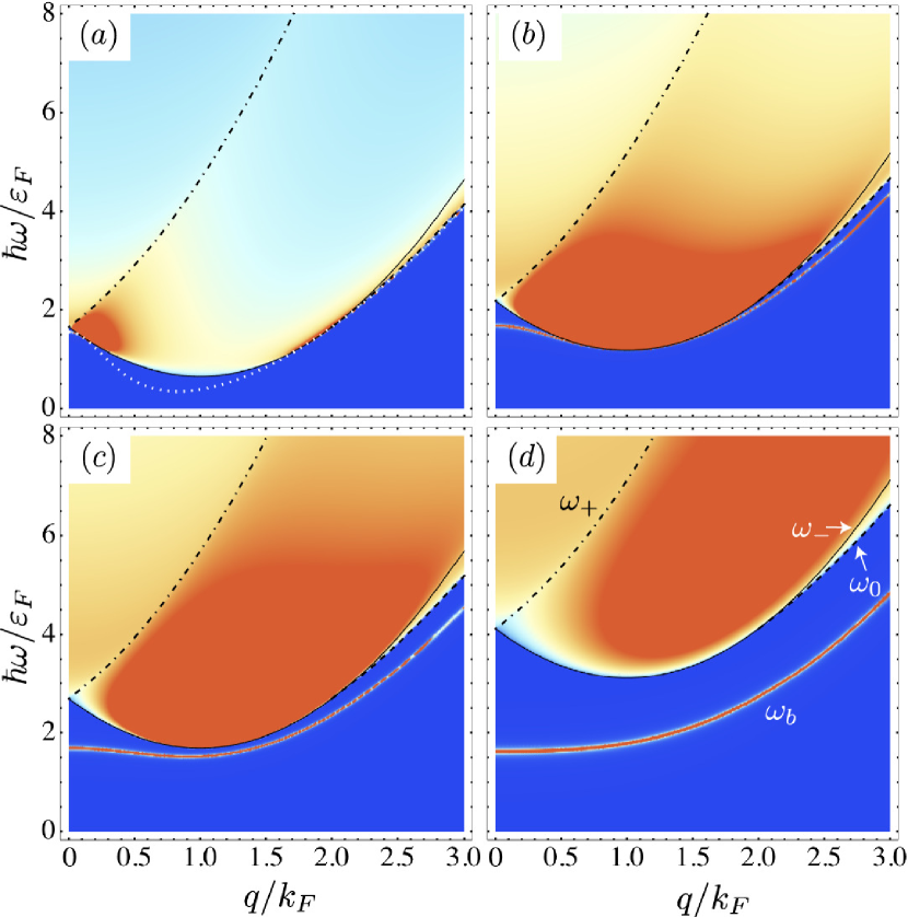
Figure 2: (color online). Molecular spectral function $\mathcal{A}_{\text{mol}}(\bm{q},\omega)$ for different values of the two-body binding energy $\varepsilon_{B}/\varepsilon_{F}$: (a) $0.1$, (b) $0.5$, (c) $1.0$, (d) $2.5$. The dashed lines mark the log continuum $\omega_{0}$, dash-dotted and solid the root continuum $\omega_{\pm}$.

In the presence of a Fermi sea of spin-$\uparrow$ atoms, the molecular state is dressed by fluctuations and described by the many-body $T$-matrix. This can be calculated in the Nozieres–Schmitt-Rink approach nozieres1985 , as done in the 2D case by Engelbrecht and Randeria engelbrecht1990 ; engelbrecht1992 . We generalize these results to the case of spin imbalance and obtain

$$T^{-1}(\bm{q},\omega)=T_{0}^{-1}(\omega+i0+\mu_{\uparrow}+\mu_{\downarrow}-\varepsilon_{\bm{q}}/2)\\ +\int\frac{d^{2}k}{(2\pi)^{2}}\,\frac{n_{F}(\varepsilon_{\bm{k}}-\mu_{\uparrow})+n_{F}(\varepsilon_{\bm{k}+\bm{q}}-\mu_{\downarrow})}{\omega+i0+\mu_{\uparrow}+\mu_{\downarrow}-\varepsilon_{\bm{k}}-\varepsilon_{\bm{k}+\bm{q}}},$$ (2)

with the Fermi function $n_{F}(\varepsilon)$. At zero temperature where $\mu_{\uparrow}=\varepsilon_{F}$ and $\mu_{\downarrow}<0$, we obtain an analytical expression for the many-body $T$-matrix

$$T(\bm{q},\omega)=T_{0}\Bigl{(}\tfrac{1}{2}z\pm\tfrac{1}{2}\sqrt{(z-\varepsilon_{\bm{q}})^{2}-4\varepsilon_{F}\varepsilon_{\bm{q}}}\Bigr{)}$$ (3)

with $z=\omega+i0-\varepsilon_{F}+\mu_{\downarrow}$ and $\pm=\operatorname{sgn}\operatorname{Re}(z-\varepsilon_{\bm{q}})$. Due to the constant density of states in 2D the many-body $T$-matrix can be expressed as the two-body $T$-matrix with the argument shifted by Pauli blocking. The molecular spectral function $\mathcal{A}_{\text{mol}}(\bm{q},\omega)=-2\operatorname{Im}T(\bm{q},\omega)$ is shown in Fig. 2 for several values of the interaction strength parametrized by the two-body binding energy $\varepsilon_{B}$. One observes a bound state peak at low energies and the particle-particle continuum at higher energies.

The continuum of dissociated molecules arises mathematically from the branch cut of the square root (3) in the region $\omega_{-}(q)<\omega<\omega_{+}(q)$, $\omega_{\pm}=\varepsilon_{F}(1\pm q/k_{F})^{2}-\mu_{\downarrow}$ (dash-dotted/solid lines), as well as from the branch cut of the logarithm (1) for $\omega>\omega_{+}(q)$ and for $\omega_{0}=\varepsilon_{\bm{q}}/2-\varepsilon_{F}-\mu_{\downarrow}<\omega<\omega_{-}(q)$ if $q>2k_{F}$ (dashed lines).

The bound state pole of the many-body T-matrix has the dispersion relation zoellner2011

$$\omega_{b}(\bm{q})=\frac{\varepsilon_{\bm{q}}/2(\varepsilon_{\bm{q}}/2-\varepsilon_{F})+\varepsilon_{B}(\varepsilon_{F}-\varepsilon_{B})}{\varepsilon_{\bm{q}}/2+\varepsilon_{B}}-\mu_{\downarrow}$$ (4)

which changes qualitatively with the two-body binding energy $\varepsilon_{B}$ (see Fig. 2): for $\varepsilon_{B}<2\varepsilon_{F}$ the bound state has minimum energy at a finite wave vector with positive effective mass $m^{*}/m=(2-2/k_{F}a_{\text{2D}})^{-1}$ suppl_mat .

Polaron and quasi-particle properties.

The impurity atom is dressed with virtual molecule-hole excitations and becomes a quasi-particle with self-energy engelbrecht1992 ; punk2007 ; suppl_mat

$$\Sigma_{\downarrow}(\bm{q},\omega)=\int_{k<k_{F}}\frac{d^{2}k}{(2\pi)^{2}}\,T(\bm{k}+\bm{q},\varepsilon_{\bm{k}}-\mu_{\uparrow}+\omega)\,,$$ (5)

which leads to the same ground state energy as a variational ansatz combescot2007 . Here we have used the fact that in the zero-temperature polaron problem the molecule has vanishing macroscopic occupation. Hence it has spectral weight only at positive frequencies (cf. Fig. 2) where the Bose distribution vanishes. We perform the integral in (5) numerically and obtain the spectral function of impurity atoms

$$\mathcal{A}_{\downarrow}(\bm{q},\omega)=-2\operatorname{Im}[\omega+i0+\mu_{\downarrow}-\varepsilon_{\bm{q}}-\Sigma_{\downarrow}(\bm{q},\omega)]^{-1}.$$ (6)

The frequency and momentum dependence of the spectral function is shown in Fig. 1 (left panel) for three values of the interaction strength. In Fig. 3 we display the zero-momentum spectral function $\mathcal{A}_{\downarrow}(q=0,E-\mu_{\downarrow})$ versus interaction parameter $\eta=\ln(k_{F}a_{\text{2D}})=-\ln(\varepsilon_{B}/2\varepsilon_{F})/2$. In both figures we set the reference energy to the free atom threshold by subtracting the chemical potential $\mu_{\downarrow}$.

At weak binding $\varepsilon_{B}\ll\varepsilon_{F}$ (Fig. 1a) the attractive polaron is a well-defined quasi-particle at small momenta but for $q\gtrsim k_{F}$ it scatters off virtual molecules and acquires a large decay width. For intermediate binding (Fig. 1b) a new repulsive polaron state appears at positive energies. It is a metastable state with broad decay width, and it is shifted to higher energy due to the repulsive interaction with the Fermi sea of spin-$\uparrow$ atoms. The dispersion of the repulsive polaron has a minimum at finite momentum $q\sim k_{F}$ reflecting a similar feature in the molecular spectral function (Fig. 2c); for larger momenta it approaches the free particle dispersion. Finally, for strong binding (Fig. 1c) both polaron branches are well separated and the repulsive polaron becomes an increasingly long-lived and stable quasi-particle. Between the attractive and the repulsive polaron branches appears the molecule-hole continuum (see also Fig. 3). Its spectral weight is small in the case of a broad Feshbach resonance studied here, but it is enhanced for narrow resonances by an admixture of closed channel molecules schmidt2011 .

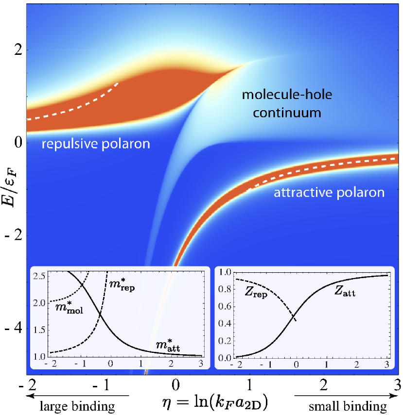
Figure 3: (color online). Polaron spectral function $\mathcal{A}_{\downarrow}(q=0,E-\mu_{\downarrow})$ versus the interaction parameter $\eta$. The dashed lines indicate the perturbation theory of Ref. bloom1975 . Left inset: effective mass $m^{*}/m$ of the attractive and repulsive polaron as well as the molecule. Right inset: crossover of the quasi-particle weight $Z$ from the repulsive to the attractive polaron.

It is instructive to see how the quasi-particle properties of the polaron change as the interaction parameter $\eta$ is varied. The right inset of Fig. 3 shows a continuous crossover where the quasi-particle weight $Z=1/[1-\partial_{\omega}\Sigma(\bm{q}=0,\omega)]$ evaluated at the quasi-particle pole, shifts from the attractive to the repulsive polaron branch: for small binding ($\eta>0$), the attractive polaron is the dominant excitation and the weight is gradually transferred toward the repulsive branch for increasing binding ($\eta<0$). This crossover is also reflected in the effective mass $m^{*}/m$ (Fig. 3 left inset). Our strong coupling calculation reproduces the perturbative results bloom1975 for the attractive and repulsive polaron energies in the weak and strong binding limits (dashed lines in Fig. 3).

Radiofrequency spectroscopy.

The spectral properties of the imbalanced Fermi gas can be accessed experimentally using rf spectroscopy. We assume that an rf pulse is used to drive atoms from an initial state $\lvert i\rangle$ to an initially empty final state $\lvert f\rangle$. We choose the final state to be strongly interacting with a bath of a third species $\lvert\uparrow\rangle$ such that $\lvert f\rangle$ is in fact the impurity state, $\lvert f\rangle=\lvert\downarrow\rangle$. This inverse rf procedure interchanges the roles of $\lvert i\rangle$ and $\lvert f\rangle$ with respect to Ref. schirotzek2009 ; it has been proposed in Refs. schmidt2011 ; massignan2011 and realized in the experiment by Fröhlich et al. froehlich2011 .

Within linear response theory, the rf transition rate is given by haussmann2009

$$I_{\text{rf}}(\omega_{\text{rf}})=-2\Omega_{\text{rf}}^{2}\operatorname{Im}\chi^{R}(-\omega_{\text{rf}}-\mu_{i}+\mu_{f})$$ (7)

where $\Omega_{\text{rf}}$ is the Rabi frequency, $\omega_{\text{rf}}$ the detuning of the rf photon from the bare transition frequency and $\mu_{i(f)}$ the initial (final) state chemical potential. The retarded correlation function $\chi^{R}$ can be computed from the corresponding time-ordered correlation function $-i\theta(t-t^{\prime})\langle[\psi_{f}^{\dagger}(\bm{r},t)\psi_{i}(\bm{r},t),\psi_{i}^{\dagger}(\bm{r}^{\prime},t^{\prime})\psi_{f}(\bm{r}^{\prime},t^{\prime})]\rangle$ punk2007 ; massignan2008 . In general vertex corrections are crucial pieri2009 ; enss2011 , but we find that they vanish in the case of negligible initial state interactions as appropriate for the experiment froehlich2011 . At $T=0$, we obtain

$$I_{\text{rf}}(\omega_{\text{rf}})=\Omega_{\text{rf}}^{2}\int_{\varepsilon_{\bm{q}}<\mu_{i}}\frac{d^{2}q}{(2\pi)^{2}}\,A_{\downarrow}(\bm{q},\omega_{\text{rf}}+\varepsilon_{\bm{q}}-\mu_{\downarrow})\,.$$ (8)

The integral in equation (8) is calculated numerically and the resulting rf spectra are shown in Fig. 1 (right panel). The rf probes the final $\lvert\downarrow\rangle$ state spectral function along the free-particle dispersion up to the initial state chemical potential $\mu_{i}$. As in the experiment froehlich2011 , we assume a balanced initial state mixture with $\mu_{i}=\mu_{\uparrow}$. We find a peak in the rf spectrum once the detuning $\omega_{\text{rf}}$ reaches the final state chemical potential $\mu_{\downarrow}$ ($\mu_{\downarrow}$ is negative in the polaron problem). The transfer of spectral weight from the attractive to the repulsive polaron can be directly observed in Fig. 1.

Comparison to experiments.

In order to relate our results to harmonically confined Fermi gases, we have to connect the strict 2D calculation to the quasi-2D geometry relevant to experiments petrov2001 ; bloch2008 . Well below the confinement energy $\hbar\omega_{z}$ where only the lowest transverse mode is occupied, this can be done by replacing $\varepsilon_{B}$ with the exact quasi-2D two-body binding energy. Thus $\varepsilon_{B}$ becomes a function of both the 3D scattering length $a_{\text{3D}}$ and the confinement length $\ell_{z}=\sqrt{\hbar/m\omega_{z}}$ (petrov2001 , cf. Eq. 82 in bloch2008 ).

Recently the quasi-2D geometry has been realized experimentally with a Fermi gas of ⁴⁰K atoms froehlich2011 . Following the inverse rf procedure described above, an initially non-interacting balanced mixture is driven into a strongly interacting final state. As long as its occupation remains small the final state is a Fermi polaron, and our calculation predicts the experimental rf response.

In Fig. 4 we show our trap averaged rf spectra versus magnetic field. We use the experimental parameters of Ref. froehlich2011 with $\omega_{z}=2\pi\times 80$ kHz, $\omega_{\perp}=2\pi\times 125$ Hz, and express $a_{\text{3D}}$ in terms of the magnetic field bloch2008 ; strohmaier2010 . We incorporate the radial trapping in the 2D plane using the local density approximation; the local Fermi energy is $\varepsilon_{F}(r)=\varepsilon_{F}-m\omega_{\perp}^{2}r^{2}/2$ with peak Fermi energy $\varepsilon_{F}=9$ kHz. Finally, we average over 30 pancakes in the $z$ direction froehlich2011 .

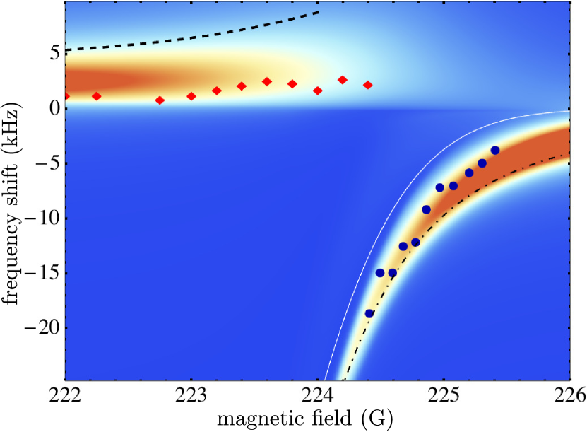
Figure 4: (color online). Trap averaged rf spectra of a quasi-2D Fermi gas: rf detuning versus magnetic field B. The experimental data points (blue and red diamonds) are taken from Ref. froehlich2011 . Also shown are the energy of the repulsive (dashed) and attractive (dash-dotted) polaron as well as the two-body binding energy (solid, white) in a homogeneous system.

We observe that the lower branch of the experimental spectra (circles) agrees well with the attractive polaron picture (Fig. 4) and our calculation provides an alternative interpretation to the two-body bound state (solid line) put forward in Ref. froehlich2011 . We note that also the measured frequency shift in 3D as shown in froehlich2011 fits the polaron picture schmidt2011 . Our results show a second rf peak at positive detunings corresponding to the repulsive polaron. The dashed line in Fig. 4 indicates its quasi-particle energy in the bulk (cf. Fig. 3). As similar for the attractive polaron energy (dash-dotted line) the trap average leads to a significant shift of the rf peaks to lower energies. The experimental data (diamonds) in this magnetic field range agrees qualitatively with our calculation. One possible reason for the remaining discrepancy is the large final state occupation in the experiment.

In conclusion, we studied Fermi polarons in two dimensions which exhibit an attractive and repulsive branch and computed their rf spectra. Additional work is needed to understand discrepancies between theory and experiment for repulsive polarons. As an example, pump and probe experiments in the form of a sequence of two short pulses may shed further light on this issue.

Supplementary material

Many-body $T$-matrix.

The molecular spectral function displayed in Fig. 2 changes qualitatively with the binding energy. For large binding $\varepsilon_{B}>2\,\varepsilon_{F}$ (Fig. 2d), the bound state (4) has minimum energy $\omega_{b}=\varepsilon_{F}-\varepsilon_{B}-\mu_{\downarrow}$ at $q=0$ and we find an effective mass $m^{*}/m\rvert_{q=0}=2/(1-2\varepsilon_{F}/\varepsilon_{B})>2$. While it is well known that the $T$-matrix does not yield the correct binding energy of the molecule in the BEC limit parish2011 the repulsive polaron, which is the focus of our work, is reproduced correctly bloom1975 . For smaller binding $\varepsilon_{B}<2\,\varepsilon_{F}$ (Fig. 2b-c), the effective mass at $q=0$ becomes negative and a new minimum appears at finite wave vector $q_{c}=2\sqrt{k_{F}a_{\text{2D}}-1}/a_{\text{2D}}$ zoellner2011 and with positive effective mass $m^{*}/m\rvert_{q=q_{c}}=(2-2/k_{F}a_{\text{2D}})^{-1}$. For decreasing binding energy $\varepsilon_{B}$ the bound state eventually touches the continuum at momenta $q_{\pm}/k_{F}=1\pm\sqrt{1-2\varepsilon_{B}/\varepsilon_{F}}$ (dotted line in Fig. 2a). For $q_{-}<q<q_{+}$ the bound state has negative residue and it ceases to exist.

Polaron self-energy.

We compute the many-body $T$-matrix in the ladder approximation which is represented diagrammatically in Fig. 5d. The self-energy of the $\downarrow$ atom is given by scattering an $\uparrow$ hole off a molecule as depicted in Fig. 5b. Explicitly, the self-energy reads

$$\Sigma_{\downarrow}^{R}(\bm{q},\omega)=\int\frac{d^{2}k}{(2\pi)^{2}}\frac{dz}{\pi}\bigl{[}n_{B}(z)G^{A}_{\uparrow}(\bm{k}-\bm{q},z-\omega)\operatorname{Im}T(\bm{k},z)\\ -n_{F}(z)\operatorname{Im}G^{R}_{\uparrow}(\bm{k},z)\,T(\bm{k}+\bm{q},z+\omega)\bigr{]}$$ (9)

where $G^{A,R}_{\uparrow}$ refers to advanced/retarded $\uparrow$ Green’s functions. The first contribution comes from the pole and branch cuts of the $T$-matrix. In the polaron problem neither the $\downarrow$ state nor the molecular state are macroscopically occupied at zero temperature, hence the molecular spectral function $\propto\operatorname{Im}T$ has weight only at positive frequencies $z>0$ where $n_{B}(z)$ vanishes, cf. Fig. 2. The second contribution of (9) with the bare $\uparrow$ spectral function $\operatorname{Im}G^{R}_{\uparrow}(\bm{k},z)=-i\pi\delta(z-\varepsilon_{\bm{k}}+\mu_{\uparrow})$ directly yields Eq. (5). The $\downarrow$ self-energy yields the $\downarrow$ Green’s function via the Dyson equation (6) depicted diagrammatically in Fig. 5c.

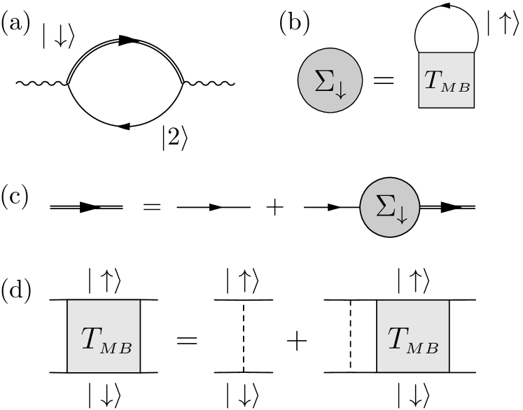
Figure 5: Diagrammatic representation of (a) the rf photon self-energy, (b) the self-energy of spin-$\downarrow$ atoms, (c) the Dyson equation for the dressed Green’s function $G_{\downarrow}$, and (d) the many-body T-matrix between states $\lvert\uparrow\rangle$ and $\lvert\downarrow\rangle$.

Local density approximation.

To incorporate the radial trapping potential we use the local density approximation (LDA). In the experiment froehlich2011 not only a single (central) 2D layer is populated but also additional pancakes along the axial direction. For each of these layers we calculate the rf response

$$I_{\text{trap}}^{(\nu)}(\omega)=\int d^{2}r\,\rho_{\text{LDA}}^{(\nu)}(\bm{r})\,I_{\text{rf}}^{(\nu)}(\omega,\bm{r}).$$ (10)

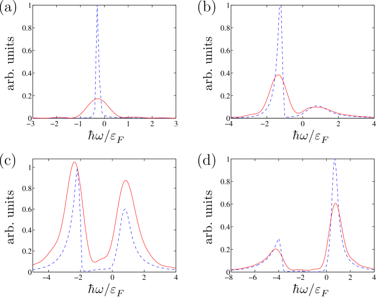
Figure 6: (color online). RF spectrum of a trapped quasi-2D Fermi gas for (a) $B=227$ G, (b) $B=225$ G, (c) $B=224.5$ G, and (d) $B=224$ G. The attractive polaron gives rise to the peak at negative frequencies and the repulsive polaron corresponds to the peak at positive frequencies. The dashed line depicts the trap averaged signal $I_{\text{trap}}$ while the solid line shows the expected experimental signal $I_{\text{exp}}$ which takes into account a rectangular rf pulse of duration $T=100\,\mu$s (not to scale) froehlich2011 .

The various pancakes are indicated by the index $\nu$ and $\rho_{\text{LDA}}^{(\nu)}(\bm{r})=m\varepsilon_{F}^{(\nu)}(r)/2\pi\hbar^{2}$ is the Thomas-Fermi distribution of the density of non-interacting fermions within a single layer. $I_{\text{rf}}^{(\nu)}(\omega,\bm{r})$ is the rf response in Eq. (8) computed for a homogeneous system with local Fermi energy $\varepsilon_{F}^{(\nu)}(r)$ and interaction parameter $\eta^{(\nu)}(r)=-\ln(\varepsilon_{B}/2\varepsilon_{F}^{(\nu)}(r))/2$. In the experiment froehlich2011 30 layers have been populated. To obtain the complete rf response of the trapped system we finally sum over 30 contributions $I_{\text{trap}}^{(\nu)}$ where we assume that the peak density of each layer, $\epsilon_{F}^{(\nu)}(0)$, varies according to a Thomas-Fermi profile along the lattice direction.

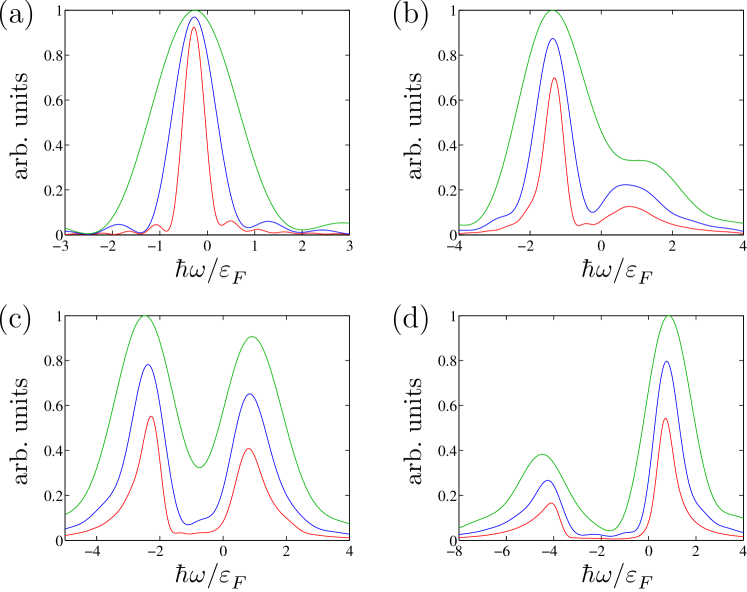
Figure 7: (color online). Same as Fig. 6 but for different rf pulse duration (from top to bottom) $T=50\,\mu$s, $T=100\,\mu$s, and $T=200\,\mu$s (not to scale).

Shape and length of the rf pulse.

The line shape of the rf spectra has a strong dependence on the rf pulse shape. The rf pulse used in Ref. froehlich2011 is approximately rectangular with duration $T=100\,\mu$s. We compute the experimental rf signal as the convolution of $I_{\text{trap}}(\omega)$ with the Fourier spectrum of the rf field haussmann2009

$$I_{\text{exp}}(\omega)=\frac{T}{2\pi}\int d\omega^{\prime}\,I_{\text{trap}}(\omega-\omega^{\prime})\,\operatorname{sinc}^{2}(\omega^{\prime}T/2).$$ (11)

In Fig. 6 we show the resulting rf spectra for different values of the external magnetic field. Note that the broadening may shift the apparent peak position, see e.g. Fig. 7b.