Many-body Landau-Zener Transition in Cold Atom Double Well Optical Lattices

Abstract

Ultra-cold atoms in optical lattices provide an ideal platform for exploring many-body physics of a large system arising from the coupling among a series of small identical systems whose few-body dynamics is exactly solvable. Using Landau-Zener (LZ) transition of bosonic atoms in double well optical lattices as an experimentally realizable model, we investigate such few to many body route by exploring the relation and difference between the small few-body (in one double well) and the large many-body (in double well lattice) non-equilibrium dynamics of cold atoms in optical lattices. We find the many-body coupling between double wells greatly enhances the LZ transition probability. The many-body dynamics in the double well lattice shares both similarity and difference from the few-body dynamics in one and two double wells. The sign of the on-site interaction plays a significant role on the many-body LZ transition. Various experimental signatures of the many-body LZ transition, including atom density, momentum distribution, and density-density correlation, are obtained.

I Introduction

Understanding many-body physics in strongly-correlated lattice models is essential for the explanation of many important condensed matter phenomena, such as the high temperature cuprate superconductivity Wen . In this context, ultra-cold atoms in optical lattices provide an ideal platform for emulating numerous phenomena in solids because of their ability of accurately implementing various lattice models without impurities, lattice phonons, and other complications Bloch2005 ; Porto ; Greiner02a ; Jaksch98 ; Duan . In solids, a large many-body system may be composed of a series of small identical few-body systems, therefore it would be natural and interesting to investigate how many-body properties (e.g. correlations) of the large system emerge or differ from the few-body properties of the small systems (see Fig. 1(a) for an illustration) Anderson . Although such few to many body route may provide a unique angle for understanding the underlying many-body physics, its experimental realization is very challenging in solids. In contrast, such route may be easily explored using the recent experimentally realized cold atom double well optical lattices Strabley06 ; Strabley07 ; Trotzky , where the few-body dynamics in each double well can be solved exactly, while the many-body physics emerges from the inter-well coupling.

The double well lattices not only allow studying interesting many-body ground states Ritt ; Salger ; ground1 ; ground2 ; ground3 ; ground4 , but also the equilibrium and non-equilibrium dynamics of cold atoms after an adiabatic or sudden change of the atom or lattice parameters Qian ; Cramer . Recently, the non-equilibrium dynamics in optical lattices after a sudden quench has been investigated intensively Cramer ; Rigol ; Kollath ; Manmana ; Moeckel ; Bernier11 ; Polkovnikov . While the dynamics for the adiabatic process is expected to follow the change of the system Hamiltonian, the goal for studying the quench dynamics is to understand the non-equilibrium physics and the relaxation to the equilibrium steady states in the presence of many-body interactions. Although the two limiting cases (adiabatic or sudden) have been widely studied, the intermediate region, that is, the parameter variation with a finite rate, has been largely unexplored Poletti ; Bernier12 ; Natu ; Clark .

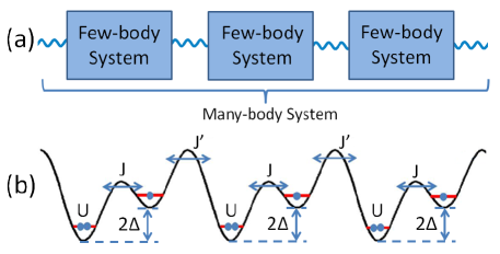
Figure 1: (Color online). (a) Illustration of the route from the few-body physics in identical small systems to the many-body physics in a large system through coupling. (b) An example for (a): the LZ transition of cold atoms in 1D double well optical lattices. The coupling between different double wells (the small systems) is provided by the inter-well coupling $J^{\prime}$.

In this paper, we integrate these two important aspects (i.e., route from few to many body physics and non-equilibrium dynamics) for cold atom optical lattices into one simple, but experimentally feasible model: the many-body Landau-Zener (LZ) transition in a one-dimensional (1D) double well optical lattice. In the LZ transition, the parameters of the Hamiltonian vary with a finite rate (neither adiabatic nor sudden), and the dynamics is naturally non-equilibrium. Furthermore, the dynamics of a single atom in an isolated double well, a classical example of the LZ transition Landau32 , is exactly solvable. Recently, the LZ transition has been generalized (both theoretically and experimentally) to a BEC in a double well (with $\sim$100 atoms per double well), where the dynamics is governed by the mean-field nonlinear interaction Wu1 ; Wu2 ; Yuao ; Kasztelan and the research focuses on the emergence of the loop structure in the energy spectrum and the invalidity of the adiabaticity.

In this paper we investigate the many-body LZ transition in a double well optical lattice to explore the route from few-body to many-body non-equilibrium dynamics. We mainly focus on the following issues: (i) the LZ transition for a few interacting atoms (in contrast to hundreds of atoms in the mean-field region Wu1 ; Wu2 ; Yuao ) in an isolated double well (i.e., without inter-well coupling); (ii) the collective LZ transition of many atoms in the double well lattice with the inter-well coupling, which has not been explored previously in the literature. Our goal is to explore the difference as well as the relation between the few-body physics in (i) and the many-body physics in (ii). We find that the onsite interaction $U$ (repulsive or attractive) between atoms can strongly modify the LZ transition in (i). For the repulsive interaction, there is an oscillation of the LZ probability with respect to $U$. In the large $U$ limit, we derive an analytical expression for the LZ transition probability using the independent crossing approximation. The inter-well tunneling that couples different double wells can significantly increase the LZ transition probability. While certain feature of the LZ transition process in a single double well is still kept in the double well optical lattice, the coherent oscillation of the transition probability in the positive $U$ region is destroyed by the many-body tunneling between double wells. We show the signature of the many-body LZ transition in various experimentally measurable quantities such as the atom density and momentum distributions, and the density-density correlation.

The rest of this paper is organized as follows: in section II we discuss the theoretical model of the experimentally realized double well optical lattice. Then we study the few-body dynamics of the LZ transition in a single double well in section III. We extend the dynamics of the LZ transition to a coupled double well lattice in section IV by switching on the inter-well coupling. In section V we discuss possible experimental signatures of many-body LZ transitions. Section VI is a summary.

II The Hamiltonian

The 1D double well lattice, schematically shown in Fig. 1(b), has been realized in many experiments by superimposing two optical lattices with different wavelengths Strabley06 ; Strabley07 ; Trotzky ; Ritt ; Salger . The dynamics along the other two dimensions is frozen to the ground states using optical lattices with high lattice potential depths. Within the tight-binding approximation, the dynamics of atoms in the 1D double well lattice is described by the Bose-Hubbard model Jaksch98 ,

$$H = -\sum\nolimits_{i}\left(Ja_{2i-1}^{{\dagger}}a_{2i}+J^{\prime}a_{2i}^{{\dagger}}a_{2i+1}+c.c.\right)$$ (1)

$$+\sum\nolimits_{i}\left(-1\right)^{i+1}\Delta n_{i}+Un_{i}\left(n_{i}-1\right),$$

where $a_{i}$ ($a_{i}^{\dagger}$) are the annihilation (creation) operators for bosons at the lattice site $i$, $n_{i}=a_{i}^{\dagger}a_{i}$, $J$ ($J^{\prime}$) represents the intra-well (inter-well) tunneling, $2\Delta=2\gamma t$ is the chemical potential difference between two neighboring lattice sites in a single double well, which varies with the time $t$ with the sweeping rate $\gamma$. $U$ is the on-site interaction strength between atoms. In experiments Strabley06 ; Strabley07 ; Trotzky , the inter- and intra-well tunnelings $J$ and $J^{\prime}$ can be adjusted independently by careful control of the intensities of the two optical lattice laser beams, the chemical potential $\Delta$ can be tuned by shifting one laser beam with respect to the other, and the on-site interaction $U$ between atoms can be changed using the Feshbach resonance. Generally the inter-well barrier, see Fig. 1(a) is larger than the intra-well barrier, i.e., $J>J^{\prime}$.

The time-dependent dynamics of atoms governed by the Hamiltonian (1) is solved numerically. Because the dimensionality of the Hamiltonian increases exponentially with respect to the lattice size, we simulate the dynamics of this system using the recently developed time-evolving block decimation (TEBD) algorithm Vidal03 ; Vidal04 ; Vidal07 ; TEBD with an open boundary condition, which is a powerful tool for studying lattice dynamics in one dimension with only nearest neighbor tunneling/interaction where the entanglement of the system is small. In our TEBD simulation, we choose the Schmidt number $\xi=20$ with at most 4 atoms at each lattice site. We have confirmed the convergence of our numerical program for the parameters used in the paper by comparing the results with that using a larger Schmidt number. For a small lattice size, we also study the dynamics using the Runge-Kutta method by including all possible configurations and find excellent agreement with the TEBD method. Henceforth, the energy unit is chosen as the intra-well tunneling $J$, and the corresponding time unit is $\hbar J^{-1}$.

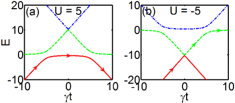
Figure 2: (Color online). Plot of the instantaneous energy levels in a single double well with two atoms. The level crossing depends strongly on the sign of $U$. The arrow indicates the time evolution of the quantum state for a relatively small sweeping rate $\gamma$.

III Few-body dynamics in one double well

For cold atoms in isolated double wells without inter-well tunneling (i.e., $J^{\prime}=0$), the probability for the atoms remaining on the same state after they pass through the LZ transition regime is known to be $\exp\left(-\pi J^{2}/\gamma\right)$ Landau32 for $U=0$. In the presence of the on-site interaction $U$ for several atoms in one double well, the LZ transition can be dramatically different because the interaction shifts the energy levels for atoms. For simplicity, we illustrate the essential physics using two atoms ($N=2$) in one double well. Under the number state basis $\left\{\left|2_{L}0_{R}\right\rangle,\left|1_{L}1_{R}\right\rangle,\left|0_{L}2_{R}\right\rangle\right\}$, the Hamiltonian can be written as

$$H_{2}=\begin{pmatrix}2\gamma t+2U&-\sqrt{2}J&0\\ -\sqrt{2}J&0&-\sqrt{2}J\\ 0&-\sqrt{2}J&-2\gamma t+2U\end{pmatrix},$$ (2)

where $L$ ($R$) represents the left (right) well. The instantaneous eigenenergy levels at the time $t$ are plotted in Fig. 2. With the large $\left|U\right|\gg J$, the two large anticrossings at $t\neq 0$ with the gap $\sim J$ yield direct LZ transitions between two quantum states that differ by exactly one atom, while the tiny anticrossing at $t=0$ with the gap $\sim J^{2}/U$ corresponds to the indirect second order transition process, which has a negligible contribution to the total LZ transition probability when the sweeping rate is faster than the time scale determined by this gap. Assuming initially the atoms are prepared on the ground state $\left|2_{L}0_{R}\right\rangle$ for $t\rightarrow-\infty$, we see for $U>0$, all atoms can be transferred from the left to the right well at $t\rightarrow+\infty$ when $\gamma$ is small (the arrow in Fig. 2(a)). While for $U\ll-J$ at most one atom can be transferred for a relatively slow sweeping rate $\gamma$ (but still fast enough such that the tiny gap at $t=0$ can be neglected). For a very small sweeping rate $\gamma$ (thus the gap at $t=0$ cannot be neglected), the dynamics is still adiabatic and all atoms can be transferred to the right well, as expected. For the atom number larger than two ($N>2$), the physical picture shown in Fig. 2 is still similar. Generally, for $U\gg J$ we observe $N$ different LZ transitions, while for $U\ll-J$ only one direct LZ transition can be found (hence at most one particle can be transferred from left to right if the sweeping rate is faster than the indirect transition gap). Finally, assuming the $i$-th LZ transition occurs at the time $t=t_{i}$ where the anticrossing between $|i,N-i\rangle$ and $|i+1,N-i-1\rangle$ takes place. At time $t_{i}$, the two states have the same energy, that is, $Ui(i-1)+U(N-i)(N-i-1)+\gamma t_{i}(i-(N-i))=Ui((i+1)-1)+U(N-(i+1))(N-(i+1)-1)+\gamma t_{i}((i+1)-(N-(i+1)))$, yielding $t_{i}=((N-1)U-2iU)/\gamma$. Therefore the time interval between two adjacent direct LZ transitions is exactly the same $\delta t=t_{i}-t_{i+1}=2U/\gamma$.

The exact time-dependent dynamics of the Hamiltonian (2) is very complex and cannot be expressed using simple analytical equations. However, simple analytical expressions for the remaining number of atoms in the left well can be derived in certain limit using the $S$-matrix method developed by Brundobler and Elser Brundobler93 , which has been successfully applied to other similar models Sinitsyn02 ; Dobrescu06 ; Volkov04 ; Sinitsyn04 ; Volkov05 ; Demkov68 ; Demkov01 ; Pokrovsky02 ; Kayanuma84 ; Pokrovsky04 ; Sinitsyn03 ; Pokrovsky07 . With the $S$-matrix method, we find

$$N_{L}=\left\{\begin{array}[]{ll}1+e^{-2\pi J^{2}/\gamma}&\quad\text{if $U\gg J$}\\ e^{-2\pi J^{2}/\gamma}(3-e^{-2\pi J^{2}/\gamma})&\quad\text{if $U\ll-J$}\\ 2e^{-2\pi J^{2}/\gamma}&\quad$U = 0$\\ &\end{array}\right.$$ (3)

using the independent crossing approximation (ICA) Brundobler93 that is valid in these limits, as shown in Fig. 2. We have verified that the above analytical results agree well with our numerical results. For $U=0$, the result reduces to the standard LZ formula Landau32 , multiplied by the total number of atoms.

IV Many-body dynamics in double well lattice

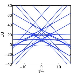
Figure 3: (Color online). Plot of the instantaneous energy levels in two coupled double wells with two atoms in each double well. $J^{\prime}=0.5J$, $U=5.0J$, $M=2$. The strong crossings and anticrossings between different quantum states make the independent crossing approximation invalid in the multiple coupled double wells.

Now we switch on the coupling $J^{\prime}$ between double wells to investigate how $J^{\prime}$ and $U$ influence the LZ transitions. To illustrate the essential physics in the large lattice, we first consider an isolated system with only two coupled double wells, each of which contains $N=2$ atoms. Similar as the Hamiltonian (2) for a single double well, we rewrite the Hamiltonian (1) to a $35\times 35$ matrix form under the number state basis $\left\{\left|i_{1}i_{2}i_{3}i_{4}\right\rangle\right\}$, where $i_{l}=\left\{0,1,2,3,4\right\}$ represents the number of atoms at the site $l$ with the constraint $i_{1}+i_{2}+i_{3}+i_{4}=4$. To gain insight into this problem, we plot the instantaneous energy levels for $U>0$ in Fig. 3. We see the ICA Brundobler93 is invalid even for a very large $U$, therefore the analytical formula for the number of atoms in the left well cannot be derived anymore. The same physical picture holds when multiple double wells in the lattice are coupled by switching on the inter-well coupling $J^{\prime}$.

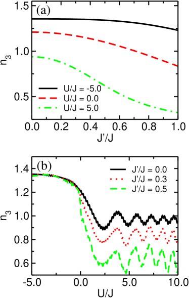
Figure 4: (Color online). Plot of the atom number $n_{3}$ in the third site versus (a) $J^{\prime}$ and (b) $U$ for two coupled double wells from the Runge-Kutta simulation. $\gamma=2\pi$.

We numerically solve the dynamics of atoms in two double wells using the fourth-order Runge-Kutta method to obtain the exact dynamics using an open boundary condition. The quantum state of the system is initially prepared at $|2_{L}0_{R}\rangle\otimes|2_{L}0_{R}\rangle$ (the ground state at $t\rightarrow-\infty$), and the number of atoms in the third site $n_{3}$ for a large positive $t$ (effectively $t\rightarrow+\infty$), i.e., the number of atoms remaining in the left well, is calculated. Note that a small $n_{3}$ means a large LZ transition probability. In Fig. 4(a), we plot $n_{3}$ as a function of $J^{\prime}$ with the finite $U$. $n_{3}$ decreases monotonically with the increasing $J^{\prime}$ for all interaction regions, which indicates the LZ transition probability is enhanced by $J^{\prime}$. This can be intuitively understood from the fact that when the inter-well tunneling is switched on, the atoms in the third site can tunnel to not only the fourth site, but also the second site.

In Fig. 4(b), we plot $n_{3}$ with respect to $U$ for finite $J^{\prime}$. We see a strong dependence of $n_{3}$ on the sign of $U$. For a large attractive $U$, $n_{3}$ is large and the LZ transition probability is small because atoms are bound together for tunneling by the large attractive interaction, as shown in Fig. 2(b). The inter-well tunneling $J^{\prime}$ barely modifies the transition probability. While in the repulsive $U$ region, $n_{3}$ decreases quickly with the increasing $U$, but saturates at the large $U$ limit. In the large $U$ region, $n_{3}$ oscillates periodically with $U$ even for $J^{\prime}=0$. Note that there are two direct LZ transitions for two atoms in a double well. After passing the minimum gap point of the first LZ transition, $n_{3}$ still oscillates periodically with time. Since the time interval between two adjacent direct LZ transitions is $\delta t=2U/\gamma$, it is expected that $n_{3}$ before the second LZ transition may oscillate with $U$, leading to the final oscillation dependence of $n_{3}$ on $U$ at $t\rightarrow+\infty$. The nonzero $J^{\prime}$ reduces $n_{3}$ significantly by enhancing the LZ transition probability. However, the positions of the peaks and valleys of the oscillation are the same for different $J^{\prime}$. Note that general analytical perturbation methods (with $J^{\prime}$ as a small parameter) do not work for the coupled LZ transition because of the non-adiabaticity and the time-dependence of the system.

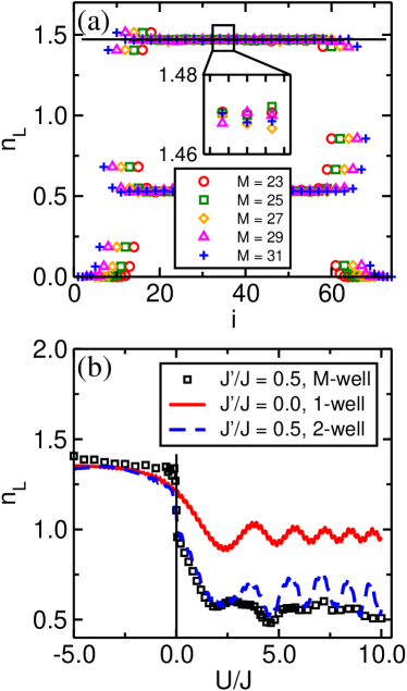
Figure 5: (Color online). (a) Plot of the atom density distribution $n_{i}$ for different lattice sizes from the TEBD simulation. $M$ is the number of double wells. $J^{\prime}=0.5J$, $U=5.0J$, $\gamma=2\pi$. An enlarged plot at the center of the lattice is shown in the inset. (b) Plot of the number of atoms at the left site $n_{L}$ of the central double well of the lattice with respect to $U$. $M=25$, and $\gamma=2\pi$.

With the knowledge of the LZ transition in single and coupled double wells, we now study the many-body LZ transitions in a lattice with many ($\sim 30$) double wells using the TEBD algorithm. Note that because of the exponentially large dimensionality of the lattice system, the fourth-order Runge-Kutta method (as well as any exact diagonalization method) is not practical. The initial wavefunction is assumed to be $|0_{L}0_{R}\rangle^{\otimes N_{L}}\otimes|2_{L}0_{R}\rangle^{\otimes M}\otimes|0_{L}0_{R}\rangle^{\otimes N_{R}}$, where $M$ is the number of occupied double wells. $N_{L}$ ($N_{R}$) is the number of unoccupied double wells at the left (right) edge of the lattice to eliminate the effects of the open boundary condition. With the finite $J^{\prime}$, the atoms may diffuse to the left and right edges in the time scale $\sim 1/J^{\prime}$. For a relatively large $\gamma$, such diffusion does not affect the LZ transition at the center of the lattice, as we show below. In the numerical simulation, we choose $N_{L}=N_{R}=3$, which are sufficient for a wide range of $\gamma$.

To check the effects of the atom diffusion on the LZ transition, we plot the number of atoms (at $t\rightarrow+\infty$) in each lattice site in Fig. 5(a) for $\gamma=2\pi$ and different $M$. Although the atom diffusion at the edge of the lattice is significant, the atom number fluctuation in the central part of the lattice is generally very small. For instance, the difference between the final atom number at the center of the lattice is smaller than $0.002$ for two different lattice sizes $M=23$ and $31$. Our numerical results show that when $M>20$ the LZ transition in the central part of the lattice can be a good approximation for that in an infinite large lattice $M\rightarrow\infty$.

We calculate the number of atoms $n_{L}$ (at $t\rightarrow+\infty$) in the left site of the double well at the center of the lattice with $M=25$, and plot it as a function of $U$ in Fig. 5(b). To compare the results with the few-body physics in the small system, we also present the results for single and two coupled double wells in the same figure. When $U<0$, $n_{L}$ is generally larger than one because of the reduced LZ transition probability by the attractive interaction. $n_{L}$ is almost the same as that in coupled double wells, which indicates $J^{\prime}$ does not modify the LZ transition significantly for the attractive interaction. For $U>0$, $n_{L}$ is generally smaller than 1. Although in a large quantum system the instantaneous eigenenergy levels become very complex, we still observe the oscillation of $n_{L}$ with respect to $U$. However, the perfect oscillation in the coupled double wells is smeared by the interference effects in lattices, leaving only one big dip at $U\simeq 4.5J$. This is very different from the coherent oscillation in one and two coupled double wells.

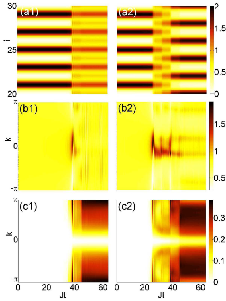
Figure 6: (Color online). Plot of the atom density $n_{i}(t)$ (a1, a2), momentum distribution $n(k,t)$ (b1, b2), and density-density correlation $s(k,t)$ (c1, c2) from TEBD numerics. $J^{\prime}=0.5J$. The left column: $U=-5J$; the right column: $U=5J$. $\gamma=2\pi$. In all panels, the dark contrast lines correspond to places for the LZ transitions (see main text for more details).

V Experimental observation

The many-body LZ transition can be observed using several different methods.

(i) The number of atoms in the left or right wells of the lattice (e.g., $n_{L}$ in Fig. 5) can be measured using the band mapping method Trotzky . In Figs. 6(a), we plot the atom density distribution during the LZ transition in the central part of the lattice. We see there is only one LZ transition for $U\ll-J$, while several LZ transitions for $U\gg J$.

(ii) When one atom is transferred from one site to the neighboring site, there should be a change of the atom momentum distribution

$$n(k,t)=\sum_{i,j}e^{ik\left(i-j\right)}\langle\psi|a_{i}^{\dagger}a_{j}|\psi\rangle,$$ (4)

which is plotted in Figs. 6(b) and can be measured using the time-of-flight image. Here $\psi\left(t\right)$ is the wavefunction obtained from the TEBD numerical simulation. Note that the actual momentum distribution may oscillate rapidly after the LZ transition, which may not be observable in experiments. Here, we take the average momentum distribution in a small time interval 0.9$\hbar J^{-1}$ in Figs. 6(b). We see the atom momentum distributions $n(k,t)$ have peaks around $k=0$ during the LZ transitions. There is a one-to-one correspondence between the density and momentum changes in the LZ transition, therefore the momentum peaks around $k=0$ (the dark lines in Figs. 6(b)) appear once for $U<0$ (one LZ transition) and several times for $U>0$.

(iii) The density-density correlation

$$s(k,t)=\sum_{i,j}e^{ik\left(i-j\right)}\left[\langle\psi|n_{i}n_{j}|\psi\rangle-\langle\psi|n_{i}|\psi\rangle\langle\psi|n_{j}|\psi\rangle\right],$$ (5)

which can be measured using the Bragg scattering Brag , shows similar features as $n_{L}$ because $n_{i}n_{j}$ should also have a sudden change in the LZ transition process. Similarily, there are different number of dark lines in Figs. 6(c) for $U<0$ and $U>0$. Note that $n(k,t)$ shows a strong asymmetry about $k=0$ because the momentum is transferred along a specific direction during the LZ transition. In contrast, the density-density correlation, due to its definition, is exactly symmetric about $k=0$. In experiments, the number of atoms in the left well $n_{L}$ and the densiy-density correlation $s(k,t)$ can also be measued using the single site detection Greiner ; Bloch3 ; Bloch4 .

Experimentally, the 1D double well lattice has been realized for ⁸⁷Rb atoms by superimposing two optical lattices with the wavelength $\lambda_{1}=\lambda_{2}/2$ and the corresponding lattice potential depths $V_{1}$ and $V_{2}$ Trotzky . The motion of atoms along the other two dimensions are frozen by two additional regular lattices with the potential depth $V_{\bot}=30E_{R}$, where $E_{R}=h^{2}/2m\lambda^{2}=2\pi\times 3.7$ KHz is the atom recoil energy. By tuning $V_{1}$ and $V_{2}$, we can set the intra-well tunneling energy $J\sim\hbar\times 2\pi\times 200$ Hz. The typical onsite interaction strength in the optical lattice is $U\sim$ $\hbar\times 2\pi\times 1$ KHz, but can be tuned using Feshbach resonance Chin10 . The chemical potential $\Delta$ can be tuned by shifting one laser beam with respect to the other Trotzky . The typical LZ transition time is $\sim$50$\hbar/J\sim 40$ ms, which can be easily achieved in experiments. Taking into account of the symmetry of the energy levels for the repulsive and attractive interactions (Figs. 2(a) and 2(b)), we can use the repulsive interaction ($U>0$) to emulate the LZ transition with the attractive interaction ($U<0$) by initially preparing the atoms in the excited state (the upper branch in Fig. 2(a)), similar as the method used in a recent experiment Trotzky .

VI Conclusion

In summary, we study the many-body effects in the LZ transition using ultra-cold bosonic atoms in 1D double well optical lattices. The dynamics of such non-adiabatic systems is obtained through large scale numerical simulations using the TEBD algorithm. Our results are important for understanding not only the route from few to many body physics when individual small systems are coupled to form a large system through the many-body coupling, but also the non-equilibrium dynamics in optical lattices when the system parameters vary with a finite rate (neither adiabatic nor sudden).

Acknowledgement: We thank Yu-Ao Chen for helpful discussion. This work is supported by ARO (W911NF-09-1-0248), DARPA-YFA (N66001-10-1-4025), and NSF (PHY-1104546).

References

- (1) P. A. Lee, N. Nagaosa, and X.-G. Wen, Rev. Mod. Phys. 78, 17 (2006).
- (2) I. Bloch, Nature Phys. 1, 23 (2005).
- (3) J. V. Porto, Nature Phys. 7, 280 (2011).
- (4) M. Greiner , O. Mandel, T. Esslinger, T. W. H’́ansch and I. Bloch, Nature 415, 39 (2002).
- (5) D. Jaksch, C. Bruder, J. I. Cirac, C. W. Gardiner and P. Zoller, Phys. Rev. Lett. 81, 3108 (1998).
- (6) L.-M. Duan, E. Demler, and M. D. Lukin, Phys. Rev. Lett. 91, 090402 (2003).
- (7) See e.g., P. W. Anderson, ”More is different”, Science, 4, 393 (1972).
- (8) J. Sebby-Strabley, M. Anderlini, P. S. Jessen and J. V. Porto, Phys. Rev. A 73, 033605 (2006).
- (9) J. Sebby-Strabley, B. L. Brown, M. Anderlini, P. L. Lee, W. D. Phillips, and J. V. Porto, Phys. Rev. Lett. 98, 200405 (2007).
- (10) S. Trotzky, P. Cheinet, S. Fölling, M. Feld, U. Schnorrberger, A. M. Rey, A. Polkovnikov, E. A. Demler, M. D. Lukin and I. Bloch, Science 319, 295 (2008).
- (11) G. Ritt, C. Geckeler, T. Salger, G. Cennini, and M. Weitz, Phys. Rev. A 74, 063622 (2006).
- (12) T. Salger, C. Geckeler, S. Kling, and M. Weitz, Phys. Rev. Lett. 99, 190405 (2007).
- (13) P. Buonsante and A. Vezzani, Phys. Rev. A 70, 033608 (2004).
- (14) I. Danshita, J. W. Williams, C. A. R. Sa de Melo, and C. W. Clark, Phys. Rev. A 76, 043606 (2007).
- (15) V. M. Stojanović, C. Wu, W. V. Liu, and S. Das Sarma, Phys. Rev. Lett. 101, 125301 (2008).
- (16) V. I. Yukalov1 and E. P. Yukalova, Phys. Rev. A 78, 063610 (2008).
- (17) Y. Qian, M. Gong, and C. Zhang, Phys. Rev. A 84, 013608 (2011).
- (18) M. Cramer, A. Flesch, I. P. McCulloch, U. Schollwock and J. Eisert, Phys. Rev. Lett. 101, 063001 (2008).
- (19) M. Rigol, V. Dunjko, V. Yurovsky and M. Oishanii, Phys. Rev. Lett. 98, 050405 (2007).
- (20) C. Kollath, A. M. Läuchli, and E. Altman, Phys. Rev. Lett. 98, 180601 (2007).
- (21) S. R. Manmana, S. Wessel, R. M. Noack and A. Muramatsu, Phys. Rev. Lett. 98, 210405 (2007).
- (22) M. Moeckel and S. Kehrein, Phys. Rev. Lett. 100, 175702 (2008).
- (23) J. S. Bernier, G. Roux, and C. Kollath, Phys. Rev. Lett. 106, 200601 (2011).
- (24) A. Polkovnikov, K. Sengupta, A. Silva and M. Vengalatore, Rev. Mod. Phys. 83, 863 (2011).
- (25) D. Poletti and C. Kollath, Phys. Rev. A 84, 013615 (2011).
- (26) J. S. Bernier, D. Poletti, P. Barmettler, G. Roux, and C. Kollath, Phys. Rev. A 85, 033641 (2012).
- (27) S. S. Natu, K. R. A. Hazzard, and E. J. Mueller, Phys. Rev. Lett. 106, 125301 (2011).
- (28) S. R. Clark and D. Jaksch, Phys. Rev. A 70, 043612 (2004).
- (29) L. Landau, Physics of the Soviet Union 2, 46 (1932); C. Zener, proceedings of the Royal Society of London A 137, 696 (1932); E. C. G. Stueckelberg, Helvetica Physica Acta 5, 369 (1932); E. Majorana, Nuovo Cimento 9, 43 (1932).
- (30) J. Liu, L. Fu, B.-Y. Ou, S.-G. Chen, D.-I. Choi, B. Wu, and Q. Niu, Phys. Rev. A 66, 023404 (2002).
- (31) B. Wu, and J. Liu, Phys. Rev. Lett. 96, 020405 (2006).
- (32) Y.-A. Chen, S. D. Huber, S. Trotzky, I. Bloch, and E. Altman, Nat. Phys. 7, 61 (2011).
- (33) C. Kasztelan, S. Trotzky, Y. -A. Chen, I. Bloch, I. P. McCulloch, U. Schollwock, and G. Orso, Phys. Rev. Lett. 106, 155302 (2011).
- (34) G. Vidal, Phys. Rev. Lett. 91, 147902 (2003).
- (35) G. Vidal, Phys. Rev. Lett. 93, 040502 (2004).
- (36) G. Vidal, Phys. Rev. Lett. 98, 070201 (2007).
- (37) see http://physics.mines.edu/downloads/software/tebd/
- (38) S. Brundobler and V. Elser, Journal of Physics A 26, 1211 (1993).
- (39) V. L. Pokrovsky and N. A. Sinitsyn, Physical Review B 65, 153105 (2002).
- (40) B. Dobrescu and N. A. Sinitsyn, Journal of Physics B 39, 1253 (2006).
- (41) M. V. Volkov and V. N. Ostrovsky, Journal of Physics B 37, 4069 (2004).
- (42) N. A. Sinitsyn, Journal of Physics A 37, 10691 (2004).
- (43) M. V. Volkov and V. N. Ostrovsky, Journal of Physics B 38, 907 (2005).
- (44) Yu. N. Demkov and V. I. Osherov, Soviet Physics JETP 24, 916 (1968).
- (45) Yu. N. Demkov and V. N. Ostrovsky, Journal of Physics B 34, 2419 (2001).
- (46) V. L. Pokrovsky and N. A. Sinitsyn, Physical Review B 65, 153105 (2002).
- (47) Y. Kayanuma, Journal of the Physical Society of Japan 53, 108 (1984).
- (48) V. L. Pokrovsky and N. A. Sinitsyn, Physical Review B 67, 045603 (2004).
- (49) N. A. Sinitsyn and N. Prokof’ev, Physical Review B 67, 134403 (2003).
- (50) V. L. Pokrovsky and D. Sun, Physical Review B 76, 024310 (2007).
- (51) J. Stenger, S. Inouye, A. P. Chikkatur, D. M. Stamper-Kurn, D. E. Pritchard and W. Ketterle, Phys. Rev. Lett. 82, 4569 (1999).
- (52) W. S. Bakr, J. I. Gillen, A. Peng, S. Foelling, M. Greiner, Nature 462, 74 (2009).
- (53) J. F. Sherson, C. Weitenberg, M. Endres, M. Cheneau, I. Bloch, and S. Kuhr, Nature 467, 68 (2010).
- (54) C. Weitenberg, M. Endres, J. F. Sherson, M. Cheneau, P. Schau, T. Fukuhara, I. Bloch, and S. Kuhr, Nature 471, 319 (2011).
- (55) C. Chin, R. Grimm, P. Julienne and E. Tiesinga, Rev. Mod. Phys. 82, 1225 (2010).