Measurement of Static and Dynamic Light Scattering

Abstract

Static Light Scattering (SLS) and Dynamic Light Scattering (DLS) are the very important techniques to study the characteristics of materials in dispersion. One fundamental application is the accurate measurement of the size distribution. SLS measures using the the optical characteristic and DLS is determined by the hydrodynamic and optical characteristics of particles in dispersion. In the theoretical analysis of DLS, the relationship between SLS and DLS is given and there exists an assumption that the static and hydrodynamic radii are equal for spherical particles and then develop some theorems to determine the structures of particles. Here, using the SLS technique, the size distribution can be measured accurately when the Rayleigh-Gans-Debye approximation is valid for dilute homogenous spherical particles in dispersion. For the commercial samples, the static sizes are consistent with the sizes provided by supplier respectively. The values of root mean square radius of gyration measured using the Zimm plot and calculated using the commercial size distributions or size distributions measured using the SLS technique are consistent respectively. Based on the static size distribution, with one assumption between the static and hydrodynamic radii, the calculated and measured data of DLS are consistent very well at all the scattering angles investigated respectively. Using the static size information the dimensionless shape parameter is discussed, our results show that the shapes can not be determined based on the dimensionless shape parameter. Traditionally, the particle information: apparent hydrodynamic radius and polydispersity index are obtained from DLS by analyzing the deviations of the intensity-intensity autocorrelation function from an exponent function. Since the apparent hydrodynamic radius obtained using the Stokes-Einstein relation is an optical weighted average radius, it is an approximate value of mean hydrodynamic radius. And the polydispersity index is not relate to the width of hydrodynamic radius. Therefore the apparent hydrodynamic radius and polydispersity index cannot give an accurate description for size distribution.

1 INTRODUCTION

Light Scattering has been considered to be a well established technique and applied in physics, chemistry, biology, etc. as an essential tool to investigate the characteristics of nanoparticles in dispersion. The treatment of Static Light Scattering (SLS) spectroscopy is simplified to the Zimm plot, Berry plot or Guinier plot etc. to get the root mean-square radius of gyration $\left\langle R_{g}^{2}\right\rangle^{1/2}$ and the molar mass of particles provided that the particle sizes are small[1, 2] and one fundamental application of Dynamic Light Scattering (DLS) technique is the accurate and fast size measurement of particles made of different materials. In general, the apparent hydrodynamic radius and polydispersity index are obtained using the method of Laplace transformation or Cumulant analysis at a given scattering angle[3, 4, 5, 6, 7]. Some researchers use the results measured using SLS and DLS together to obtain much more information of nanoparticles [8, 9, 10, 11, 12]. Although people have proposed the theoretical function of the normalized time electric field auto-correlation function of the scattered light $g^{\left(1\right)}(\tau)$[4, 6, 13] and try to obtain more information about nanoparticles using SLS and DLS together, the comparison of the expected values and experimental data of the normalized time auto-correlation function of the scattered light intensity $g^{\left(2\right)}\left(\tau\right)$ has not been detailed.

How the particle size distribution can be obtained directly from SLS data has been reported. Strawbridge and Hallett[14] studied the theoretical scattered intensity of coated spheres with vertically polarized incident light. The scattered intensity at the geometrical or linear trial radii between $r_{\min}$ and $r_{\max}$ was used to fit SLS data. Schnablegger and Glatter[15] assumed that the size distribution can be described as a series of cubic B-splines and used the simulated and measured data to demonstrate the computation procedure.

For dilute homogeneous spherical particles in dispersion, one method[19] are used to obtain the accurate static size distribution. The number distribution of particles is chosen as a Gaussian distribution and the effects of the scattering vector and the different intensity weights of different particle sizes on the scattered light intensity are considered. With the assistance of a non-linear least square fitting program, the mean static radius $\left\langle R_{s}\right\rangle$ and standard deviation $\sigma$ are measured accurately. For the polystyrene spherical particles investigated, the values of mean static radius and mean radius measured using Transmission Electron Microscopy (TEM) technique provided by the supplier are consistent.

Based on the particle size distribution measured using SLS technique, DLS technique was investigated further. The expected values of $g^{\left(2\right)}\left(\tau\right)$ calculated based on the SLS measurements or commercial results provided by the supplier are consistent with the experimental data very well. This result also reveals that the static and hydrodynamic radii of spherical nanoparticles are different and have a large difference.

In order to obtain more information about particles, some people believe that there exist some relationships between the physical quantities obtained using SLS and DLS techniques. A lot of people believe that the dimensionless shape parameter ${\left\langle{R_{g}}^{2}\right\rangle^{\frac{1}{2}}}/{R_{app,h}}$ can give a good description of the shapes of particles. However based on our results, the dimensionless shape parameter is ${\left\langle{R_{g}}^{2}\right\rangle^{\frac{1}{2}}}/{\left\langle{R_{s}}\right\rangle}$. Therefore without the knowledge about the relationship of mean static and apparent hydrodynamic radii, this dimensionless shape parameter ${\left\langle{R_{g}}^{2}\right\rangle^{\frac{1}{2}}}/{R_{app,h}}$ cannot be determined.

2 THEORY

When the homogeneous spherical particles are considered and Rayleigh-Gans-Debye(RGD) approximation is valid, the average scattered light intensity of a dilute non-interacting system in unit volume can be obtained for vertically polarized light

$$\frac{I_{s}}{I_{inc}}=\frac{4\pi^{2}\sin^{2}\theta_{1}n_{s}^{2}\left(\frac{dn}{dc}\right)_{c=0}^{2}c}{\lambda^{4}r^{2}}\frac{4\pi\rho}{3}\frac{\int_{0}^{\infty}R_{s}^{6}P\left(q,R_{s}\right)G\left(R_{s}\right)dR_{s}}{\int_{0}^{\infty}R_{s}^{3}G\left(R_{s}\right)dR_{s}},$$ (1)

where $\theta_{1}$ is the angle between the polarization of the incident electric field and the propagation direction of the scattered field, $c$ is the mass concentration of particles, $r$ is the distance between the scattering particle and the point of intensity measurement, $\rho$ is the density of particles, $I_{inc}$ is the incident light intensity, $I_{s}$ is the intensity of the scattered light that reaches the detector, $R_{s}$ is the static radius of a particle, $\ q=\frac{4\pi}{\lambda}n_{s}\sin\frac{\theta}{2}$ is the scattering vector, $\lambda$ is the wavelength of incident light in vacuo, $n_{s}$ is the solvent refractive index, $\theta$ is the scattering angle, $P\left(q,R_{s}\right)$ is the form factor of homogeneous spherical particles

$$P\left(q,R_{s}\right)=\frac{9}{q^{6}R_{s}^{6}}\left(\sin\left(qR_{s}\right)-qR_{s}\cos\left(qR_{s}\right)\right)^{2}$$ (2)

and $G\left(R_{s}\right)$ is the number distribution of particles. In this work, the number distribution is chosen as a Gaussian distribution

$$G\left(R_{s};\left\langle R_{s}\right\rangle,\sigma\right)=\frac{1}{\sigma\sqrt{2\pi}}\exp\left(-\frac{1}{2}\left(\frac{R_{s}-\left\langle R_{s}\right\rangle}{\sigma}\right)^{2}\right),$$ (3)

where $\left\langle R_{s}\right\rangle$ is the mean static radius and $\sigma$ is the standard deviation.

If the reflected light is considered, the average scattered light intensity in unit volume is written as

$$\frac{I_{s}}{I_{inc}}=a\frac{4\pi\rho}{3}\frac{\int_{0}^{\infty}R_{s}^{6}P\left(q,R_{s}\right)G\left(R_{s}\right)dR_{s}+b\int_{0}^{\infty}R_{s}^{6}P\left(q^{\prime},R_{s}\right)G\left(R_{s}\right)dR_{s}}{\int_{0}^{\infty}R_{s}^{3}G\left(R_{s}\right)dR_{s}}$$ (4)

where

$$a=\frac{4\pi^{2}\sin^{2}\theta_{1}n_{s}^{2}\left(\frac{dn}{dc}\right)_{c=0}^{2}c}{\lambda^{4}r^{2}}$$ (5)

and

$$q^{\prime}=\frac{4\pi}{\lambda}n_{s}\sin\frac{\pi-\theta}{2}$$ (6)

is the scattering vector of the reflected light. $b$ is a constant determined by the shape of sample cell, the refractive indices of solvent and the sample cell and the geometry of instruments.

For dilute homogeneous spherical particles, $g^{\left(1\right)}(\tau)$ can be obtained

$$g^{\left(1\right)}\left(\tau\right)=\frac{\int R_{s}^{6}P\left(q,R_{s}\right)G\left(R_{s}\right)\exp\left(-q^{2}D\tau\right)dR_{s}}{\int R_{s}^{6}P\left(q,R_{s}\right)G\left(R_{s}\right)dR_{s}},$$ (7)

where $D$ is the diffusion coefficient.

From the Stokes-Einstein relation

$$D=\frac{k_{B}T}{6\pi\eta_{0}R_{h}},$$ (8)

where $\eta_{0}$, $k_{B}$ and $T$ are the viscosity of solvent, Boltzmann’s constant and absolute temperature respectively, the hydrodynamic radius $R_{h}$ can be obtained.

In this work, the relationship between the static and hydrodynamic radii is assumed to be

$$R_{h}=kR_{s},$$ (9)

where $k$ is a constant. From the Siegert relation between $g^{\left(2\right)}\left(\tau\right)$ and $g^{\left(1\right)}\left(\tau\right)$ [7]

$$g^{\left(2\right)}\left(\tau\right)=1+\beta\left(g^{\left(1\right)}\right)^{2},$$ (10)

the function between SLS and DLS is built and the values of $g^{\left(2\right)}\left(\tau\right)$ can be expected based on the particle size information measured using SLS technique.

Traditionally for a solution of noninteracting monodisperse particles $g^{\left(1\right)}\left(\tau\right)$ has this form

$$g^{\left(1\right)}\left(\tau\right)=exp{\left(-\Gamma\tau\right)}$$ (11)

where $\Gamma=q^{2}D$ is the decay rate, $D$ is the macromolecular translational diffusion coefficient of the particles. For a polydisperse system, $g^{\left(1\right)}\left(\tau\right)$ consists of a distribution of exponentials

$$g^{\left(1\right)}\left(\tau\right)=\int{G{\left(\Gamma\right)}exp{\left(-\Gamma\tau\right)}d\Gamma}$$ (12)

where $G{\left(\Gamma\right)}$ is the normalized distribution of the decay rates. The size distribution can be obtained using the method of moment analysis. The mean decay rate $\overline{\Gamma}$ and the moments of the distribution $\mu_{2}$ are defined as

$$\overline{\Gamma}=\int{\Gamma G{\left(\Gamma\right)}d\Gamma}$$ (13)

$$\mu_{2}=\int{{\left(\Gamma-\overline{\Gamma}\right)}^{2}G{\left(\Gamma\right)}d\Gamma}$$ (14)

The apparent hydrodynamic radius $R_{app,h}$ is defined using the Stokes-Einstein relation[20]

$$D=\frac{k_{B}T}{6\pi\eta_{0}R_{app,h}}=\overline{\Gamma}/q^{2},$$ (15)

The polydispersity index is defined as

$$PD.I=\frac{\mu_{2}}{{\overline{\Gamma}}^{2}}.$$ (16)

A dimensionless shape parameter $\rho$ of particles is defined as

$$\rho={\left\langle{R_{g}}^{2}\right\rangle^{\frac{1}{2}}}/{R_{app,h}}$$ (17)

For a long time, the measurements of $\rho$ are used to infer particle shapes.

3 EXPERIMENT

The SLS and DLS data were measured using the instrument built by ALV-Laser Vertriebsgesellschaft m.b.H (Langen, Germany). It utilizes an ALV-5000 Multiple Tau Digital Correlator and a JDS Uniphase 1145P He-Ne laser to provide a 23 mW vertically polarized laser at wavelength of 632.8 nm.

In this work, two kinds of samples were used. One is Poly($N$-isopropylacrylamide) (PNIPAM) submicron spheres. $N$-isopropylacrylamide (NIPAM, monomer) from Acros Organics was recrystallized from hexane/acetone solution. Potassium persulfate (KPS, initiator) and $N,N^{\prime}$-methylenebi-sacrylamide (BIS, cross-linker) from Aldrich were used as received. Fresh de-ionized water from a Milli-Q Plus water purification system (Millipore, Bedford, with a 0.2 $\mu m$ filter) was used throughout the experiments. The synthesis of gel particles was described elsewhere[16, 17] and the recipes of the batches used in this work are listed in Table 3. The three samples are named according to the molar ratios $n_{B}/n_{N}$ of $N,N^{\prime}$-methyle-nebisacrylamide over $N$-isopropylacrylamide.

Sample	T (oC)	$t$ (hrs)	$W_{N}+W_{B}$ (g)	$KPS$ (mg)	$n_{B}/n_{N}$
PNIPAM-1	$70\pm 1$	$4.0$	$1.00$	$40$	$1.0\%$
PNIPAM-2	$70\pm 1$	$4.0$	$1.00$	$40$	$2.0\%$
PNIPAM-5	$70\pm 1$	$4.0$	$1.00$	$40$	$5.0\%$

Table 1: Synthesis conditions for PNIPAM particles.

The three PNIPAM samples were centrifuged at 14,500 RPM followed by decantation of the supernatants and re-dispersion in fresh de-ionized water. The process was repeated four times to remove of free ions and any possible linear chains. Then the samples were diluted for light scattering to weight factors of $8.56\times 10^{-6}$, $9.99\times 10^{-6}$ and $8.38\times 10^{-6}$ for PNIPAM-1, PNIPAM-2 and PNIPAM-5 respectively. 0.45 $\mu m$ filters (Millipore, Bedford) were used to clarify the samples before light scattering measurements. The other kind of samples is two standard polystyrene latex samples from Interfacial Dynamics Corporation (Portland, Oregon). One polystyrene sample is the sulfate polystyrene latex with a normalized mean radius of 33.5 nm (Latex-1) and the other is the surfactant-free sulfate polystyrene latex of 55 nm (Latex-2), as shown in Table 2. Latex-1 and Latex-2 were diluted for light scattering to weight factors of $1.02\times 10^{-5}$ and $1.58\times 10^{-5}$ respectively.

4 DATA ANALYSIS

In this section, how to measure the particle size distribution using SLS technique and the comparison of the expected values and experimental data of $g^{\left(2\right)}\left(\tau\right)$ are shown.

4.1 Standard polystyrene latex samples

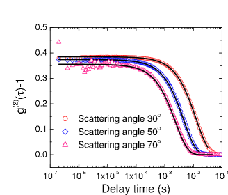
Figure 4: The experimental data and expected values of $g^{\left(2\right)}\left(\tau\right)$ for PNIPAM-1 at a temperature of 302.33 K. The symbols show the experimental data and the lines show the expected values calculated under $R_{h}=1.21R_{s}$.

The particle size information was provided by the supplier as obtained using TEM technique. Because of the small particle sizes and the large difference between the refractive indices of the polystyrene latex (1.591 at wavelength 590 nm and 20 ^oC) and the water (1.332), i.e., the “phase shift” $\frac{4\pi}{\lambda}R|m-1|$ [6, 18] are 0.13 and 0.21 for Latex-1 and Latex-2 respectively, which do not exactly satisfy the rough criterion for validity of the RGD approximation[6], the mono-disperse model $G\left(R_{s}\right)=\delta\left(R_{s}-\left\langle R_{s}\right\rangle\right)$ was used to measure the approximate values of $\left\langle R_{s}\right\rangle$ for the two polystyrene latex samples, respectively. The values of the mean radii and standard deviations of the two samples shown in Table 2 were input into Eq. 1 to get $I_{s}/I_{inc}$ respectively. In order to compare with the experimental data, the calculated value was set to be equal to that of the experimental data at $q=0.0189$ nm^-1 for Latex-1. This results and fitting results for Latex-2 are shown in Figs. 4.1a and 4.1b, respectively. The results show that the value measured using SLS technique is consistent with that measured using TEM technique.

$\left\langle R\right\rangle_{comm}$ (nm)	$\sigma_{comm}$ (nm)	$\left\langle R_{s}\right\rangle$ (nm)
33.5(Latex-1)	2.5	33.3$\pm$0.2
55(Latex-2)	2.5	56.77$\pm$0.04

Table 2: The average radius measured using TEM and SLS techniques.

$\begin{array}[]{c@{\hspace{0in}}c}\includegraphics[width=145.99367pt,angle={-90}]{Poly33cal.eps}&\includegraphics[width=145.99367pt,angle={-90}]{Poly55fit.eps}\\[0.0pt] \end{array}$

Figure 1: a). The experimental data and expected values of $I_{s}/I_{inc}$ for Latex-1 and b). The fitting results for Latex-2. In a, the circles show the experimental data and the line represents the expected values of $I_{s}/I_{inc}$. In b, the circles show the experimental data and the line shows the fitting results.

If the constant $k$ in Eq. 9 is assumed to be 1.1 for Latex-1 and 1.2 for Latex-2 and the size information provided by the supplier is assumed to be consistent with that measured using SLS technique, all the experimental data and expected values of $g^{\left(2\right)}\left(\tau\right)$ at the scattering angles 30^o, 60^o, 90^o, 120^o and 150^o and a temperature of 298.45 K for Latex-1, 298.17 K for Latex-2 are shown in Figs. 4.1a and 4.1b, respectively. Figure 4.1 shows that the expected values are consistent with the experimental data very well.

$\begin{array}[]{c@{\hspace{0in}}c}\includegraphics[width=145.99367pt,angle={-90}]{Poly33DLScal.eps}&\includegraphics[width=145.99367pt,angle={-90}]{Poly55DLScal.eps}\\[0.0pt] \end{array}$

Figure 2: The experimental data and expected values of $g^{\left(2\right)}\left(\tau\right)$. a). for Latex-1 and b). for Latex-2. The symbols show the experimental data and the lines show the expected values calculated under $R_{h}=kR_{s}$.

4.2 PNIPAM samples

When Eq. 1 was used to fit the SLS data of PNIPAM-1 measured at a temperature of 302.33 K, it was found that the results of $\left\langle R_{s}\right\rangle$ and $\sigma$ depend on the scattering vector range being fit, as shown in Table 4.2. If a small scattering vector range is chosen, the parameters are not well-determined. As the scattering vector range is increased, the uncertainties in the parameters decrease and $\left\langle R_{s}\right\rangle$ and $\sigma$ stabilize. If the fit range continues to increase, the values of $\left\langle R_{s}\right\rangle$ and $\sigma$ begin to change and $\chi^{2}$ grows. This is due to the deviation between the experimental and theoretical scattered light intensity in the vicinity of the scattered intensity minimum around $q=0.0177$ nm^-1, where most of the scattered light is cancelled due to the light interference. A lot of properties of nanoparticles could influence the scattered light intensity in this region. For example, the number distribution of particles deviates from a Gaussian distribution, the particle shapes deviate from a perfect sphere and the density of particles deviates from homogeneity, etc. In order to avoid the influences of light interference, the stable fit results $\left\langle R_{s}\right\rangle=254.3\pm 0.1$ nm and $\sigma=21.5\pm 0.3$ nm obtained in the scattering vector range from 0.00345 to 0.01517 nm^-1 are chosen as the size information measured using SLS technique. The stable fit results and the residuals in the scattering vector range from 0.00345 to 0.01517 nm^-1 are shown in Fig. 4.2.

$q$ ($10^{-3}$ nm-1)	$\left\langle R_{s}\right\rangle$ (nm)	$\sigma$ (nm)	$\chi^{2}$
3.45 to 9.05	260.09$\pm$9.81	12.66$\pm$19.81	1.64
3.45 to 11.18	260.30$\pm$1.49	12.30$\pm$3.37	1.65
3.45 to 13.23	253.45$\pm$0.69	22.80$\pm$0.94	2.26
3.45 to 14.21	254.10$\pm$0.15	21.94$\pm$0.36	2.03
3.45 to 15.17	254.34$\pm$0.12	21.47$\pm$0.33	2.15
3.45 to 17.00	255.40$\pm$0.10	17.32$\pm$0.22	11.02

Table 3: The fit results obtained using Eq. 1 for PNIPAM-1 at different scattering vector ranges and a temperature of 302.33 K.

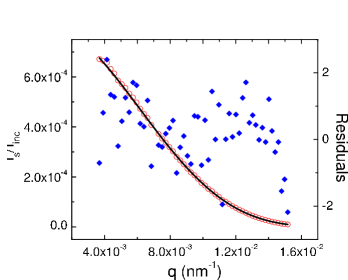
Figure 3: The experimental data and stable fit results obtained using Eq. 1 for PNIPAM-1 at a temperature of 302.33 K. The circles show the experimental data, the line shows the fit results and the diamonds show the residuals: $\left(y_{i}-y_{fit}\right)/\sigma_{i}$.

When the reflected light was considered, Eq. 4 was used to fit the data in the full scattering vector range (0.00345 to 0.0255 nm^-1) for the various factors of reflected light $b$. The fit results are listed in Table 4.2. The results show that the values of $\chi^{2}$ are much larger. The mean static radius $\left\langle R_{s}\right\rangle$ is consistent with that measured using Eq. 1 in the scattering vector range from 0.00345 to 0.01517 nm^-1 and the standard deviation changes to smaller.

$b$	$\left\langle R_{s}\right\rangle$ (nm)	$\sigma$ (nm)	$\chi^{2}$
0.01	254.0$\pm$0.3	14.4$\pm$0.5	194.60
0.011	254.0$\pm$0.3	14.6$\pm$0.5	168.20
0.012	254.0$\pm$0.3	14.7$\pm$0.5	149.99
0.013	254.0$\pm$0.2	14.8$\pm$0.4	139.82
0.014	254.1$\pm$0.2	15.0$\pm$0.4	137.52
0.015	254.1$\pm$0.2	15.1$\pm$0.4	142.96
0.016	254.09$\pm$0.07	15.2$\pm$0.5	155.97
0.017	254.1$\pm$0.3	15.4$\pm$0.5	176.40
0.018	254.1$\pm$0.3	15.5$\pm$0.5	204.08

Table 4: The fit results for PNIPAM-1 obtained from Eq. 4 using the various values of $b$.

As discussed above, light interference in the vicinity of the scattered intensity minimum would influence the fit results. In order to eliminate the effects of light interference, the experimental data in the vicinity of the scattered intensity minimum were neglected. Eq. 4 was thus used to fit the experimental data in the full scattering vector range again. The fit values are listed in Table 4.2. The mean static radius and standard deviation are consistent with the stable fit results obtained using Eq. 1 in the scattering vector range from 0.00345 to 0.01517 nm^-1.

$b$	$\left\langle R_{s}\right\rangle$ (nm)	$\sigma$ (nm)	$\chi^{2}$
0.013	251.3$\pm$0.6	22.17$\pm$0.05	79.80
0.014	251.1$\pm$0.6	23.3$\pm$0.9	58.29
0.015	250.9$\pm$0.6	24.4$\pm$0.8	44.50
0.016	250.7$\pm$0.5	25.4$\pm$0.7	37.02
0.017	250.5$\pm$0.6	26.4$\pm$0.7	36.01
0.018	250.3$\pm$0.6	27.24$\pm$0.8	41.59

Table 5: The fit results for PNIPAM-1 obtained using Eq. 4 and neglecting experimental data near the intensity minimum.

If the constant $k$ in Eq. 9 for the PNIPAM-1 is assumed to be 1.21, all the experimental data and expected values of $g^{\left(2\right)}\left(\tau\right)$ at the scattering angles 30^o, 50^o and 70^o are shown in Fig. 4.2. Figure 4.2 shows that the expected values are consistent with the experimental data very well.

For the PNIPAM samples at high temperatures, the situation using Eq. 1 is the same as that of PNIPAM-1 at a temperature of 302.33 K. The values of $\left\langle R_{s}\right\rangle$ and $\sigma$ depend on the scattering vector range being fit. If a small scattering vector range is chosen, the parameters are not well-determined. As the scattering vector range is increased, the uncertainties in the parameters decrease and $\left\langle R_{s}\right\rangle$ and $\sigma$ stabilize. The stable fit results $\left\langle R_{s}\right\rangle=139.3\pm 0.3$ nm and $\sigma=12.4\pm 0.6$ nm obtained in the scattering vector range from 0.00345 to 0.02555 nm^-1 for PNIPAM-5 at a temperature of 312.66 K are chosen as the size information measured using SLS technique. Figure 4.2a shows the stable fit results and the residuals. If the constant $k$ in Eq. 9 for PNIPAM-5 is assumed to be 1.1, all the experimental and expected values of $g^{\left(2\right)}\left(\tau\right)$ at the scattering angles 30^o, 50^o, 70^o and 100^o are shown in Fig. 4.2b. The expected values of $g^{\left(2\right)}\left(\tau\right)$ are consistent with the experimental data very well.

$\begin{array}[]{c@{\hspace{0in}}c}\includegraphics[width=145.99367pt,angle={-90}]{PNIhTfit.eps}&\includegraphics[width=145.99367pt,angle={-90}]{PNIhTcal.eps}\\[0.0pt] \end{array}$

Figure 5: The results of PNIPAM-5 at a temperature 312.66 K. a). The experimental data and stable fit results obtained using Eq. 1. The circles show the experimental data, the line shows the fit results and the diamonds show the residuals: $\left(y_{i}-y_{fit}\right)/\sigma_{i}$. b). The experimental data and expected values of $g^{\left(2\right)}\left(\tau\right)$. The symbols show the experimental data and the lines show the expected values calculated under $R_{h}=1.1R_{s}$.

5 RESULTS AND DISCUSSION

Same conclusions are also obtained for all other samples investigated. The fit results of $\left\langle R_{s}\right\rangle$ and $\sigma$ depend on the scattering vector range being fit. If a small scattering vector range is chosen, the parameters are not well-determined. As the scattering vector range is increased, the uncertainties in the parameters decrease and $\left\langle R_{s}\right\rangle$ and $\sigma$ stabilize.

For the PNIPAM samples, the main reason for the difference between experimental and theoretical scattered intensity in the vicinity of the scattered intensity minimum seems to be that the small and large particles in solution do not exist. With the mean static radius and standard deviation obtained using Eq. 1 in the $q$ range between 0.00345 and 0.01517 nm^-1, three different ways of calculation were performed to explore which can give the best expectation of the experimental data. In Fig. 5, the expected values of the scattered intensity related to incident intensity were first calculated from Eq. 1 in the full particle size distribution range between 1 and 800 nm. The calculated curve (solid line) matches the experimental date points only when q is smaller than 0.016 nm^-1. Then, a truncated Gaussian distribution was used and the calculation was performed between $\left\langle R_{s}\right\rangle-1.3\sigma$ and $\left\langle R_{s}\right\rangle+1.3\sigma$ using Eq. 1. The calculated curve (dash line) matches the experimental date points in a broader $q$ range including the vicinity of the scattered intensity minimum and deviates only at $q\geq 0.021$ nm^-1 where the reflected light could be detected. Finally, the integrated range did not change but the reflected light was considered and Eq. 4 was used to calculate the expected results assuming $b=0.014$. The calculated curve (dot line) matches the experimental date in all $q$ range investigated. The results show that the scattered intensity in the vicinity of the scattered intensity minimum is very sensitive to the particle size distribution and the influences of the reflected light only lies at very large scattering vectors.

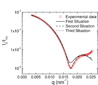
Figure 6: The experimental data and expected values for PNIPAM-1 at a temperature of 302.33 K. The circles show the experimental data, the solid line shows the expected values calculated using Eq. 1 in the full particle size distribution range, the dash line represents the expected values calculated using Eq. 1 between $\left\langle R_{s}\right\rangle-1.3\sigma$ and $\left\langle R_{s}\right\rangle+1.3\sigma$ and the dot line shows the expected values calculated using Eq. 4 in the same range as the second with $b$: $0.014$.

For the DLS measurements of all the samples investigated, the expected values calculated based on the particle size distribution measured using SLS technique or commercial results provided by the supplier are consistent with the experiment data very well, respectively. All the results reveal that the static and hydrodynamic radii are different.

In general, the apparent hydrodynamic radius and polydispersity index are two important parameters that people try to measure accurately from DLS measurements. People also believe that the small values of polydispersity index mean the size distribution of nanoparticles is narrow or monodisperse and the apparent hydrodynamic radius is equal to the mean hydrodynamic radius. Since the apparent hydrodynamic radius and polydispersity index of particles are obtained through detecting nonexponentility of the correlation function of temporal fluctuation in the scattered light at a given scattering angle, so the effects of particle size distribution and scattering angle on the nonexponentility of the correlation function of temporal fluctuation in the scattered light were investigated.

For simplicity, the difference between the static and hydrodynamic radii of homogeneous spherical particles does not be considered. The apparent hydrodynamic radius ${R_{app,h}}$ and polydispersity index $PD.I$ obtained using the Cumulant method at a given scattering vector $q$ as $\tau\rightarrow 0$ are given by

$${R_{app,h}}=\frac{\int_{0}^{\infty}R_{s}^{6}P\left(q,R_{s}\right)G\left(R_{s}\right)dR_{s}}{\int_{0}^{\infty}R_{s}^{5}P\left(q,R_{s}\right)G\left(R_{s}\right)dR_{s}}$$ (18)

and

$$PD.I=\frac{\int_{0}^{\infty}R_{s}^{4}P\left(q,R_{s}\right)G\left(R_{s}\right)dR_{s}\int_{0}^{\infty}R_{s}^{6}P\left(q,R_{s}\right)G\left(R_{s}\right)dR_{s}}{\left(\int_{0}^{\infty}R_{s}^{5}P\left(q,R_{s}\right)G\left(R_{s}\right)dR_{s}\right)^{2}}-1.$$ (19)

The values of ${R_{app,h}}$ and $PD.I$ for the mean hydrodynamic radius 5 nm with different standard deviations at scattering angles 0^o, 30^o, 60^o, 90^o and 120^o are shown in Figs. 5a and 5b, respectively. For all the calculation, the wavelength of the incident light in vacuo $\lambda$ is set to 632.8 nm and solvent refractive index $n_{s}$ is 1.332.

$\begin{array}[]{c@{\hspace{0in}}c}\includegraphics[width=145.99367pt,angle={-90}]{RhRadiusS.eps}&\includegraphics[width=145.99367pt,angle={-90}]{PDIS.eps}\\[0.0pt] \end{array}$

Figure 7: a). The apparent hydrodynamic radius and b). polydispersity index as a function of relative standard deviation at scattering angles 0^o, 30^o, 60^o, 90^o and 120^o for the nanoparticles with mean hydrodynamic radius 5 nm.

Figure 5a shows that the apparent hydrodynamic radius is greatly affected by the relative standard deviation and can have a very large difference with mean hydrodynamic radius. When the relative standard deviation is less than 1, the effect of scattering angle can be ignored. At any scattering angle, the apparent hydrodynamic radius can be measured accurately. Figure 5b reveals that polydispersity index almost does not be affected by the scattering angle and approximates a constant 0.1 when the value of relative standard deviation is larger than 3.

The situation for large particles with mean hydrodynamic radius 100 nm also was investigated. ${R_{app,h}}$ and $PD.I$ as a function of relative standard deviation at scattering angles 0^o, 30^o, 60^o, 90^o and 120^o are shown in Figs. 5a and 5b, respectively.

$\begin{array}[]{c@{\hspace{0in}}c}\includegraphics[width=145.99367pt,angle={-90}]{RhRadiusL.eps}&\includegraphics[width=145.99367pt,angle={-90}]{PDIL.eps}\\[0.0pt] \end{array}$

Figure 8: a). The apparent hydrodynamic radius and b). polydispersity index as a function of relative standard deviation at scattering angles 0^o, 30^o, 60^o, 90^o and 120^o for the nanoparticles with mean hydrodynamic radius 100 nm.

Figure 5a not only shows that the values of apparent hydrodynamic radius are greatly affected by the relative standard deviation, but also reveals the complex effects of scattering angle on ${R_{app,h}}$. Even if the values of apparent hydrodynamic radius measured at different scattering angles are consistent, it still does not mean the particle size distribution is narrow or monodisperse. In order to measure accurately the values of apparent hydrodynamic radius, the experimental data must be measured at enough small scattering angles. Figure 5b shows the same situation as Figure 5b for the polydispersity index of apparent hydrodynamic radius. As the relative standard deviation is increased, the polydisperse index approximates a constant 0.1.

For the polystyrene latex sample, all the results obtained using the different techniques are shown in Table 5.

$R_{TEM}$(nm)	$\left\langle R_{s}\right\rangle$(nm)	$R_{app,h}$ (nm)	$R_{app,h}/\left\langle R_{s}\right\rangle$
33.5	33.3$\pm$0.2	37.27$\pm$0.09	1.119$\pm$0.007
55	56.77$\pm$0.04	64.5$\pm$0.6	1.14$\pm$0.01
90	92.05$\pm$0.04	103.1$\pm$0.4	1.120$\pm$0.004

Table 6: The commercial $R_{TEM}$, $\left\langle R_{s}\right\rangle$ apparent hydrodynamic radii.

Based on the results above, the sizes obtained using SLS technique are consistent with the commercial values obtained using TEM respectively. The value of the apparent hydrodynamic radius obtained under the same conditions as the static radius is larger than that of the static radius by about $12\%$.

The values of the root mean square radius of gyration ${\left\langle{R_{g}}^{2}\right\rangle}^{1/2}_{cal}$ calculated using the commercial size distribution are consistent with the measured values of ${\left\langle{R_{g}}^{2}\right\rangle}^{1/2}_{Zimm}$ obtained from the Zimm plot analysis. All the results are shown in Table 5.

Sample	${\left\langle{R_{g}}^{2}\right\rangle}^{1/2}_{cal}$	${\left\langle{R_{g}}^{2}\right\rangle}^{1/2}_{Zimm}$
33.5(nm)	26.9	26.9$\pm$0.5
55 (nm)	43.24	46.8$\pm$0.3
90 (nm)	70.1	69.0$\pm$2.0

Table 7: Values of ${\left\langle{R_{g}}^{2}\right\rangle}^{1/2}_{cal}$ and ${\left\langle{R_{g}}^{2}\right\rangle}^{1/2}_{Zimm}$.

Based on the discussion above, the size distribution obtained using the SLS is more accurate to represent the particle information in dispersion and consistent with that measured using the TEM technique. The apparent hydrodynamic radius is an optical weight hydrodynamic radius, so it contains much more information of particle in dispersion comparing with static radius. The ratio of $R_{app,h}/\left\langle R_{s}\right\rangle$ can be larger than 2. The results for PNIPAM samples are also shown in Table 5. The results also reveal the same situation that the size distribution obtained using the SLS is more accurate to represent the particle information in dispersion.

Sample (Temperature)	$\rho$	${\left\langle{R_{g}}^{2}\right\rangle}^{1/2}_{Zimm}/\left\langle R_{s}\right\rangle$	${\left\langle{R_{g}}^{2}\right\rangle}^{1/2}_{cal}/\left\langle R_{s}\right\rangle$
PNIPAM-5($40^{o}$C)	0.73$\pm$0.02	0.83$\pm$0.03	0.813$\pm$0.003
PNIPAM-2($40^{o}$C)	0.69$\pm$0.03	0.84$\pm$0.04	0.82$\pm$0.01
PNIPAM-1($40^{o}$C)	0.69$\pm$0.03	0.87$\pm$0.04	0.856$\pm$0.009
PNIPAM-0($40^{o}$C)	0.66$\pm$0.01	0.80$\pm$0.02	0.81$\pm$0.01
PNIPAM-0($34^{o}$C)	0.54$\pm$0.02	1.13$\pm$0.03	1.04$\pm$0.03

Table 8: The values of the dimensionless parameters of $\rho$, ${\left\langle{R_{g}}^{2}\right\rangle}^{1/2}_{Zimm}/\left\langle R_{s}\right\rangle$ and ${\left\langle{R_{g}}^{2}\right\rangle}^{1/2}_{cal}/\left\langle R_{s}\right\rangle$.

6 CONCLUSION

Using the Eq. 1, the accurate size distribution of static radii $R_{s}$ can be measured using the SLS technique. Since the size distributions of polystyrene latex samples obtained using the TEM and SLS techniques are consistent and the values of the root mean square radius of gyration ${\left\langle{R_{g}}^{2}\right\rangle}^{1/2}_{cal}$ calculated using the commercial size distribution or static size distributions are consistent with the measured values of ${\left\langle{R_{g}}^{2}\right\rangle}^{1/2}_{Zimm}$ obtained using the Zimm plot analysis respectively, the size distribution obtained using the SLS is more accurate to represent the particle information in dispersion. The static and hydrodynamic radii describe the distinct characteristics of particles in dispersion, so they are different physical quantities and can have very large difference. With the SLS and DLS techniques together, the much more information about the particles in dispersion can be explored further. Using the SLS technique to study different shape particles in dispersion, the results of research maybe can improve our understanding for the scattering light from the particles in dispersion totally. The apparent hydrodynamic radius and polydispersity index cannot give an accurate description for size distribution.

References

- [1] Zimm B H 1948 J. Chem. Phys. 16 1099.
- [2] Burchard W 1983 Adv. Polym. Sci. 48 1.
- [3] Koppel D E 1972 J. Chem. Phys. 57 4814.
- [4] Bargeron C B 1974 J. Chem. Phys. 61 2134.
- [5] Brown J C, Pusey P N and Dietz R 1975 J. Chem. Phys. 62 1136.
- [6] Berne B J and Pecora R Dynamic Light Scattering (Robert E. Krieger Publishing Company, Malabar, Florida, 1990).
- [7] Brown W Dynamic Light Scattering: The Method and Some Applications (Clarendon Press, Oxford, 1993).
- [8] Bryant G, Martin S, Budi A and van Megen W 2003 Langmuir 19 616.
- [9] Burchard W, Kajiwara K and Nerger D 1982 J. Polym. Sci. 20 157
- [10] Burchard W, Schmidt M and Stockmayer W H 1980 Macromolecules 13 1265.
- [11] Hu T and Wu C 1999 Phys. Rev. Lett. 83 4105.
- [12] Wu J, Huang G and Hu Z 2003 Macromolecules 36 440.
- [13] Pusey P N and van Megen W 1984 J. Chem. Phys. 80 3513.
- [14] Strawbridge K B and Hallett F R 1994 Macromolecules 27 2283
- [15] Schnablegger H and Glatter O 1993 J. Colloid Interface Sci. 158 228.
- [16] Gao J and Frisken B J 2003 Langmuir 19 5217.
- [17] Gao J and Frisken B J 2003 Langmuir 19 5212.
- [18] van de Hulst H C Light Scattering by Small Particles (Dover Publications, Inc. New York, 1981).
- [19] Sun Y C Different Particle Size Information Obtained From Static and Dynamic Laser Light Scattering (Thesis, Simon Fraser University, 2004).
- [20] The ALV Manual of the version for ALV-5000/E for Windows, ALV-Gmbh, Germany, 1998.