Coherent vortex structures in quantum turbulence

Abstract

This report addresses an important question discussed by the quantum turbulence community during the last decade: do quantized vortices form, in zero-temperature superfluids, coherent structures similar to vortex tubes in ordinary, viscous turbulence? So far the evidence provided by numerical simulations is that bundles of quantized vortices appear in finite-temperature superfluids, but from the interaction with existing coherent structures in the turbulent (viscous) normal fluid, rather than due to the intrinsic superfuid dynamics. In this report we show that, in very intense quantum turbulence (whose simulation was made possible by a tree algorithm), the vortex tangle contains small coherent vortical structures (bundles of quantized vortices) which arise from the Biot–Savart dynamics alone, and which are similar to the coherent structures observed in classical viscous turbulence.

It has been known since the 1980’s that homogeneous isotropic turbulence contains intermittent worm-like regions of concentrated vorticity Siggia ; Kerr ; Sreeni85 ; Douady ; Moffatt ; Sreeni-Antonia ; Moisy-Jimenez . Their role in the dynamics of turbulence is not clear Frisch : there is no consensus as to whether they are responsible for the main properties of turbulence (e.g the celebrated Kolmogorov energy spectrum) or only affect the tails of statistical distributions and the exponents of high-order structure functions. Turbulence is also studied at temperatures near absolute zero in superfluid helium Vinen ; Manchester ; Lancaster ; Helsinki . Here the viscosity is zero, and the vorticity is concentrated in thin, discrete vortex lines of fixed core radius and circulation (whereas vortices in ordinary fluids are viscous and can have any size and strength). This ‘quantum turbulence’ shares important properties with the ordinary (classical) turbulence Vinen ; Skrbek ; Lvov_2006 , from the same drag force on a moving sphere VanSciver to the Kolmogorov energy spectrum in homogeneous isotropic turbulence Tabeling ; Grenoble ; Nore ; Tsubota-vd ; Tsubota-GP ; Baggaley-density . Here we show that, alongside the Kolmogorov spectrum, quantized vortices tend to form coherent structures, similar to the vortex tubes of ordinary turbulence. Despite its relative simplicity, quantum turbulence seems to share important features of generic turbulent flows.

At temperatures $T$ below $0.7\,\rm K$, thermal excitations become ballistic (in that sense that their propagation is not affected by any interaction with the background) so that liquid ⁴He is effectively a pure superfluid. Because of the quantum-mechanical constraints on the rotation, its flow is everywhere potential with the exception of vortex line singularities of atomic thickness (the core radius is approximately $a_{0}\approx 0.1\,\rm nm$), each line carrying one quantum of circulation $\kappa=h/m=10^{-7}\,\rm m^{2}/s$, where $h$ is Planck’s constant and $m$ is the mass of the single helium atom. (In liquid ³He-B, which becomes superfluid at much lower temperatures, $T<1\,{\rm mK}$, the core radius is about $80\,{\rm nm}$, and the quantum of circulation is $\kappa=h/(2m)=0.662\times 10^{-7}\,\rm m^{2}/s$, where $m$ is the atomic mass of the ³He isotope, whose nuclei are fermions.) Quantum turbulence, readily created by stirring the liquid helium, takes the form of an apparently disordered tangle of such vortex lines. The question which we ask is whether discrete quantized vortex filaments organize themselves and form coherent structures, as in ordinary turbulence.

To model quantum turbulence in the zero-temperature limit, we observe that $a_{0}$ is many orders of magnitude smaller than the typical distance, $\ell\approx 10^{-4}$–$10^{-6}\,\rm m$, between vortex lines in experiments, so it is appropriate to describe vortex lines as space curves ${\bf s}(\xi,t)$ of infinitesimal thickness which move according to the Biot–Savart law Saffman

$$\frac{d{\bf s}}{dt}=-\frac{\kappa}{4\pi}\oint_{\cal L}\frac{({\bf s}-{\bf r})}{|{\bf s}-{\bf r}|^{3}}\times{\bf dr},$$ (1)

where ${\bf s}$ is the position vector of a point on the vortex line, $t$ is time, $\xi$ is the arc length measured along the vortex line, and the integral extends over the entire vortex configuration $\cal L$. Equation (1) states classical incompressible Euler dynamics in integral form. However, unlike classical Euler vortices, quantized vortices reconnect if they come sufficiently close to each other, as seen directly in recent experiments Maryland and demonstrated using the Gross–Pitaevskii equation for the Bose–Einstein condensate Koplik . To apply equation (1) to superfluid helium we must therefore add an algorithmic reconnection procedure Schwarz .

We perform numerical simulations of reconnecting vortex lines at $T=0$ evolving according equation (1) in a period cubic box of the size $D=0.75\times 10^{-3}\,\rm m$. The technique to discretize the vortex lines, the regularization of the Biot–Savart integral, and the vortex reconnection procedure are standard and well described in the literature Schwarz ; Tsubota-vd . Our numerical algorithm, which controls the discretization, enforces a separation $\Delta\xi$ between points on the vortex line to remain between $2\times 10^{-6}\,\rm m$ and $4\times 10^{-6}\,\rm m$ during the evolution; this is therefore the numerical resolution of the computation. The time integration uses a third-order Adams–Bashforth scheme; the typical time step is $\Delta t=4\times 10^{-6}\,\rm s$. Our vortex reconnection procedure guarantees that a small amount of vortex length (as a proxy for kinetic energy) is lost at each reconnection, in agreement with numerical calculations of vortex reconnections performed using the Gross–Pitaevskii equation Leadbeater . The reconnection procedure and the enforcement of the minimum distance $\Delta\xi$ provide the numerical dissipation mechanism which plays the rôle of phonon emission in actual ⁴He Baggaley-cascade (or of the Caroli–Matricon Kopnin mechanism in ³He-B). To cope with the large number $N\sim 10^{5}$ of discretization points along the vortex lines, we use a tree algorithm Barnes ; Baggaley-density ; Baggaley-long which reduces the CPU time needed to evaluate the Biot–Savart integrals from $N^{2}$ to $N\log{N}$. The initial condition consists of randomly oriented straight vortex lines, each carrying one quantum of circulation (however, we checked that results do not depend on the initial configuration of vortices). We find that the initial vortices interact and reconnect, and, after a transient of the order of $0.03\,\rm s$, the vortex line density (vortex length per unit volume) saturates at the average value $L=7.9\times 10^{8}\,\rm m^{-2}$. The average curvature saturates too. The vortex tangle is shown in Figure 1. By construction, the circulation of each vortex line is conserved, and each vortex moves exclusively due to the collective influences of all the other vortex lines; this represents an accurate model of quantum turbulence.

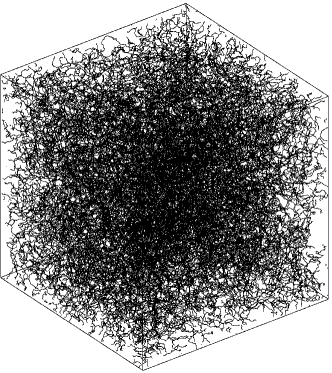
Figure 1: The instantaneous form of the saturated vortex tangle at $t=0.06\,\rm s$.

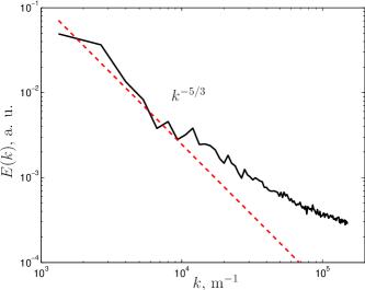
Figure 2: The energy spectrum $E(k)$ for the flow of Figure 1. The red dashed line shows the classical Kolmogorov scaling $k^{-5/3}$.

One of the most important quantity in theory of turbulence is the energy spectrum, $E(k)$ defined by

$$E=\frac{1}{V}\int_{V}{\textstyle{\frac{1}{2}}}|{\bf{v}}|^{2}\,dV=\int_{0}^{\infty}E(k)\,dk\,,$$ (2)

where $E$ is the kinetic energy (per unit mass), $V$ is volume, $k=|{\bf{k}}|$, with ${\bf{k}}$ the wave vector. Figure 2 shows a spectrum typical of quantum turbulence. The Biot–Savart interactions of vortex lines over length scales larger than the average inter-vortex distance $\ell\approx L^{-1/2}$ has induced the same Kolmogorov energy spectrum $E(k)\sim k^{-5/3}$ (for $k\ll k_{\ell}=2\pi/{\ell}$) which is observed in ordinary turbulence . The Kolmogorov spectrum was also observed in experiments with turbulent superfluid helium Tabeling ; Grenoble , and in calculations performed with both the vortex filament model Tsubota-vd ; Baggaley-density and the Gross–Pitaevskii equation Nore ; Tsubota-GP . At larger wavenumbers the spectrum becomes shallower due to the Kelvin-wave cascade along individual vortex lines Baggaley-cascade ; Kozik ; Lvov , in agreement with Refs. Tsubota-vd ; Sasa . The Kelvin cascade (which is not the main concern in this work) is due to the nonlinear interaction of Kelvin waves (helical perturbations of vortex filaments). It transfers kinetic energy downscale, creating shorter and shorter waves, until, at very short length scales, phonon emission turns the kinetic energy of the waves into the sound energy. (In ³He-B, the dissipation in the zero-temperature limit is likely to be associated with a different, Caroli-Matricon mechanism of energy loss from Kelvin waves into the quasiparticle bound states.) In our calculation, a small numerical dissipation arising from the discretization and the vortex reconnection procedure plays the role of phonon emission Baggaley-cascade . If we continued the calculation for a longer time, this numerical dissipation would make the vortex length to decay, but the energy and the length can be considered effectively constant over the timescale of interest here.

To highlight the presence of any structure in the vortex tangle shown in Figure 1, we convolve our discrete vortex filaments with a Gaussian kernel, and define a smoothed vorticity field $\omega$ as

$${\mbox{\boldmath$\omega$}}({\bf{r}},\,t)=\kappa\sum_{i=1}^{N}\frac{{\bf{s}}^{\prime}_{i}}{(2\pi\sigma^{2})^{3/2}}\exp(-|{\bf{s}}_{i}-{\bf{r}}|^{2}/2\sigma^{2})\Delta\xi\,,$$ (3)

where ${\bf{s}}^{\prime}_{i}=d{\bf{s}}_{i}/d\xi$ is the unit vector along a vortex at the discretization point ${\bf{s}}_{i}={\bf{s}}_{i}(\xi,t)$, and the smoothing length $\sigma$ is of the order of $\ell$. We test that, under this smoothing operation, a collection of randomly oriented vortex lines whose separation is of the order of $\ell$ yields ${\mbox{\boldmath$\omega$}}\approx{\bf 0}$; conversely, an organized bundle of vortex filaments of the same circulation yields a smooth vorticity distribution. Because of the wigglyness of the vortex lines at short lengthscales created by the Kelvin cascade, we also test the smoothing procedure on vortex lines after adding ten helical waves with an imposed $k^{-7/5}$ Kelvin-wave amplitude spectrum, as shown in Figure 3.

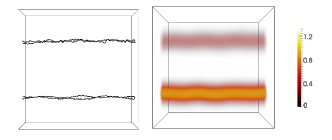
Figure 3: Volume rendering (a semi-transparent representation) of the magnitude of the smoothed vorticity field $|{\mbox{\boldmath$\omega$}}({\bf{r}})|,\,{\rm s}^{-1}$, from antiparallel (top) and parallel (bottom) vortex pairs. In the former, the average vorticity is small but not zero due to the presence of small-amplitude Kelvin waves (note the wigglyness of the vortex filaments). In the latter, the contributions of the two vortex strands add up.

Figure 4 shows the smoothed vorticity corresponding to Figure 1: vortical ‘worms’, such as those seen in numerical simulations of ordinary turbulence, are clearly visible.

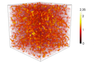
Figure 4: Volume rendering of the magnitude of the smoothed vorticity field of Figure 1, $|{\mbox{\boldmath$\omega$}}({\bf{r}})|,\,{\rm s}^{-1}$. Note the vortical worm-like structures, similar to the coherent structures observed in ordinary turbulence.

This is clear evidence of three-dimensional coherent superfluid vortex structures at $T=0$ which arise simply by the fundamental equation of motion (1) of vortex dynamics. There have been reports on the existence of vortex bundles Kivotides ; Morris in Biot–Savart simulations of quantum turbulence at relatively high temperatures, $0.7\,{\rm K}<T<T_{\lambda}\approx 2.17\,{\rm K}$, where thermal excitations form a viscous normal fluid component which interacts with the vortex lines via the mutual friction force. However, in this finite-temperature regime, vortical structures belong to the normal turbulent fluid, and the friction force Hulton would naturally induce superfluid bundles around them (although their stability is an open question). Here we focus on the development of vortical bundles in the perfect superfluid, as a consequence of pure incompressible Euler dynamics. An intermittent vortex structure has also been noticed in a recent Sasa Gross–Pitaevskii simulation of turbulence in a Bose–Einstein condensate. However, in their calculation the vortex cores were (typically of a Bose–Einstein condensate, either realized numerically or in the laboratory) very close to each other: $\ell/a_{0}\approx 4.5$ to $9$, in contrast to our much larger $\ell/a_{0}\approx 3.5\times 10^{3}$ typical of ⁴He and ³He-B superfluids; compressible effects (rapid density changes near vortex cores, sound waves, and the application of artificial damping which affects vortex positions) which are absent in our (incompressible) Biot–Savart model were also likely to have played a rôle.

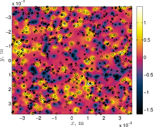
Figure 5: The cross-section $z=0$ of the $z$-component of the smoothed vorticity field from Figure 4, $\omega_{z}({\bf{r}}),{\rm s}^{-1}$. Open circles show where vortex lines cross the plane from $z<0$, and asterisks show those coming from $z>0$. The clustering of vortex points of the same sign is evident, visible as regions of large positive and negative smoothed values of $\omega_{z}$ (shown blue and yellow).

To verify that the structures in Figure 4 are indeed bundles of quantized vortices, we show in Figure 5 a two-dimensional cross-section of the $z$-component of the smoothed vorticity $\omega$ in the $z=0$ plane of Figure 4. We overlay the intersections of vortex filaments with the plane $z=0$ distinguishing the sign of $\omega_{z}$. It is apparent that the smoothed vortical structures shown in Figure 4 are indeed small bundles of aligned vortex filaments, which appear as small clusters of positive and negative vorticity. There are typically 2 to 5 vortex points in each cluster.

It is important to check that the vortex bundles are physically distinct coherent structures of a well-defined scale, rather than just a part of a purely random distribution, which would also contain structures of any scale which would become prominent after averaging. Clustering in any two-dimensional system of points (or of any other discrete objects) can be confirmed and quantified using Ripley’s $K$-function Ripley , or, alternatively, Besag’s $L$-function Besag . These functions, frequently used in applied statistics, were also used to detect spatial correlations in two-dimensional physical systems (in particular in Monte-Carlo simulations and also in biological applications of the Ising model). Ripley’s $K$-function is defined as

$$K(d)=\left(\frac{D}{M}\right)^{2}\sum_{i=1}^{M}\sum_{j=1,j\neq i}^{M}I(d_{i,j}<d)\,,$$ (4)

where $M$ is the number of points within the area $A=D^{2}$ (with $D$ the size of the domain), $d_{i,j}$ is the distance between points $i$ and $j$, and the $I(x)$ is unity if the condition $x$ is satisfied and zero otherwise. However, the related Besag’s function is more convenient for our purposes, defined as

$$L(d)=\sqrt{K(d)/\pi}-d\,;$$ (5)

$L=0$ means complete spatial randomness, $L<0$ implies dispersion, and $L>0$ aggregation (clustering). We show in Figure 6 Besag’s function for a large collection of two-dimensional cross-sections of Figure 4. The result confirms that vortex points of the same sign tend to cluster, hence the vortex bundles of Figure 4 represent distinct physical entities rather than merely an element of a purely random distribution of vorticity.

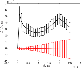
Figure 6: Besag’s function, $L(d)$, averaged over a random selection of 1,000 two-dimensional cross-sections (parallel to one of the coordinate planes) of the vortex tangle of Figure 4 in the final, statistically steady state (black) and the initial state (red). Vertical bars show the one standard deviation range. Note that $L$ increases with $d$ sharply from $L=0$ at $d=0$ to its maximum value for $d\approx 4\times 10^{-6}\,{\rm m}$, and then varies smoothly with $d$, reaching the secondary maximum at $d\approx 2\times 10^{-3}\,\rm m$. The fact that in the final state$L(d)$ is significantly larger than zero, in the whole range of $d$ explored, confirms the existence of coherent structures (clusters of vortex filaments in each cross-section) of various scales $d$, with some predominance of $d\approx 2\times 10^{-3}\,\rm m$. On the contrary, the initial state has $L=0$ within errors at all scales, consistently with the purely random nature of the initial conditions.

We now proceed with the interpretation of our results, paying particular attention to the relation to the ordinary turbulence. According to our calculations, parallel vortex lines tend to come together locally, forming clusters of vortex filaments of the same circulation in any cross-section through the flow. If the vorticity distribution was two-dimensional, the well-known inverse enstrophy cascade of the two-dimensional turbulence would transfer vorticity to large scales, creating large-scale regions populated by vortices of the same sign. The two-dimensional inverse cascade is due to the conservation of the enstrophy, $Q=\int_{V}|{\mbox{\boldmath$\omega$}}|^{2}\,dV$, the second invariant of the Euler equation in two dimensions. In three dimensions, only the first integral exists, the kinetic energy $E=\int_{V}{\textstyle{\frac{1}{2}}}|{\bf{v}}|^{2}\,dV$, whose conservation results in the direct cascade of the energy to smaller scales in both two- and three-dimensional turbulent flows.

To find whether there is a link between formation of three-dimensional coherent structures and tendency of vortices to cluster in two dimensions we performed additional numerical experiments. The two-dimensional system of interacting point vortices in the inviscid fluid was introduced by Onsager Onsager in 1949, and is known as the Onsager point-vortex gas. This is where the concept of inverse cascade was born. Onsager found that, statistically, the states of the two-dimensional system corresponding to the formation of large-scale coherent structures (clusters of point vortices of the same polarity) formally have negative temperature (a detailed analysis was later provided by Montgomery Montgomery ). The ordering of vortices and the properties of the inverse cascade in the point-vortex gas have been extensively studied, with the numerical study of the formation of large-scale circulation patterns in the two-dimensional periodic domain by Montgomery and Joyce Montgomery-Joyce being one of the first studies of this kind. Recently some of the authors of the present report demonstrated Wang the clustering of point vortices of the same polarity in a small system of just a few hundred vortices, by computing the dis balance between the vortices and antivortices within subdomains of the periodic two-dimensional computational domain. Here we have simulated the evolution of a much larger number (10,000) of point vortices in two dimensions. The system evolves from a statistically uniform state with zero net circulation where the number of vortices equals that of antivortices. Using Besag’s function, we have confirmed quantitatively the non-random clustering of vortex points.

To check if coherent structures discussed above could be a fossil of the two-dimensional reverse cascade that survives in three dimensions, we explored a modified two-dimensional Onsager’s system of point vortices similar to that shown in Figure 5. We modelled the vortex motion out of the plane by removing randomly chosen vortex-antivortex pairs from the plane at a certain rate, and then randomly re-introducing them at random positions elsewhere in the plane. For example, if a moving vortex loop in three dimensions crosses the plane, the number of point vortices in the plane first increases by two, and then is reduced by two as the loop leaves the plane. As these disturbances violate the local enstrophy conservation, they can be used to model, in a heuristic manner, local three-dimensional effects. We found that Besag’s function in such a disturbed two-dimensional system still shows tendency to clustering typical of the inverse enstrophy cascade, but weaker than in the pure two-dimensional case. The (positive) value of Besag’s function depends on the rate of vortex removal. It is therefore likely that the two-dimensional tendency to cluster is limited by the fact that the enstrophy is not constant, but this tendency is not entirely suppressed entirely.

When interpreting our results, it is also useful to compare them with recent calculations of Numasato et al. Numasato , who observed only the direct energy cascade in a two-dimensional Bose–Einstein condensate. These authors solved the Gross–Pitaevskii equation; this model allows vortex reconnections, hence does not conserve the number of vortices (i.e., the enstrophy). These authors also argued that the Gross–Pitaevskii model is compressible (the condensate’s density vanishes at the vortex axes and large-scale sound waves are easily excited, as noticed by White et al. White ), and the compressibility alone could explain the lack of the inverse cascade. Can compressibility be equally important in our case? As we already noted above, in a typical atomic Bose–Einstein condensate, either realized numerically or in the laboratory, the distance between the vortices, $\ell$, is only a few times larger than the vortex core radius $a_{0}$, while $\ell/a_{0}=O(10^{4})$ in the superfluid helium. Therefore, compressibility is less likely to prevent the formation of coherent structures in the superfluid turbulence.

In the ordinary turbulence, the origin of coherent vorticity structures is often attributed to the roll-up of vortex sheets by the Kelvin–Helmholtz instability Vincent-Meneguzzi1994 . The superfluid turbulence considered here has no vortex sheets, so the coherent structures observed here seem to involve a different mechanism.

Our future work will explore if the number of vortex lines in the bundles increases as the circulation is reduced (with kinetic energy fixed), as one expects that the limit $h\to 0$ should yield the classical behaviour where the range of vorticity values in coherent structures is wider than that observed in our numerical experiments. To better understand the dynamics of coherent structures, we also plan to investigate the time evolution of Ripley’s and Besag’s functions for the three-dimensional vortex tangle and to explore the time correlations of the flow.

In summary, our numerical experiments with very intense quantum turbulence at absolute zero have revealed that the vortex tangle contains coherent vortical structures, or bundles of vortex lines, which arise from the Biot–Savart dynamics alone, and appear to be similar to the vorticity ‘worms’ observed in the ordinary turbulence. This result sheds new light on the relation between the ordinary and quantum turbulent flows, suggesting that their connection can be deeper than usually assumed. Given the relative simplicity of the quantum turbulence, this may provide new insights into the nature of turbulence.

- (1) Siggia ED (1981). Numerical study of small scale intermittency in three-dimensional turbulence. J Fluid Mech 107: 375–406.
- (2) Kerr RM ( 1985). Higher order derivative correlations and the alignment of small scale structures in isotropic numerical turbulence. J Fluid Mech 153: 31–58.
- (3) Sreenivasan KR (1985). Transition and turbulence in fluid flows and low dimensional chaos. Frontiers in Fluid Mechanics, ed. by Davis SH and Lumley JL (Springer-Verlag, New-York), pp. 41–67.
- (4) Douady S, Coudet Y, and Brachet ME (1991). Direct observation of the intermittency of intense vorticity filaments in turbulence. Phys Rev Lett 1991: 983–986.
- (5) Moffatt HK, and Kida S (1994). Stretched vortices, the sinews of turbulence, large Reynolds number asymptotics. J Fluid Mech 259: 241–264.
- (6) Sreenivasan KR, and Antonia, RA (1997). The phenomenology of small-scale turbulence. Ann Rev Fluid Mech 29: 435–472.
- (7) Moisy F, and Jimenez J (2004). Geometry and clustering of intense structures in isotropic turbulence. J Fluid Mech 513: 111–133.
- (8) Frisch U (1995). Turbulence. The legacy of A.N. Kolmogorov (Cambridge University Press, Cambridge).
- (9) Vinen WF, and Niemela JJ (2002). Quantum turbulence. J Low Temp Phys 128: 167–231.
- (10) Walmsley PM, and Golov AI (2008). Quantum and quasiclassical types of superfluid turbulence. Phys Rev Lett 100: 245301.
- (11) Bradley DI et al. (2011). Direct measurement of the energy dissipated by quantum turbulence. Nature Physics 7: 473–476.
- (12) Eltsov VB et al. (2007). Quantum turbulence in a propagating superfluid vortex front. Phys Rev Lett 99: 265301
- (13) Skrbek L (2006). A flow phase diagram for helium superfluids. JETP Lett 80: 474–478.
- (14) L’vov VS, Nazarenko SV, and Skrbek L (2006). Energy spectra of developed turbulence in helium superfluids. J Low Temp Phys 145: 125–142.
- (15) Smith MR, Hilton DK, and Van Sciver SW (1999). Observed drag crisis on a sphere in flowing He I and He II. Phys Fluids 11: 751–753.
- (16) Maurer J, and Tabeling P (1998). Local investigation of superfluid turbulence. Europhys Lett 43: 29–34.
- (17) Salort J et al. (2010). Turbulent velocity spectra in superfluid flows. Phys Fluids 22: 125102.
- (18) Nore C, Abid M, and Brachet ME (1997). Kolmogorov turbulence in low-temperature superflows. Phys Rev Lett 78: 3896–3899.
- (19) Araki T, Tsubota M, and Nemirovskii SK (2002). Energy spectrum of superfluid turbulence with no normal-fluid component. Phys Rev Lett 89: 145301.
- (20) Kobayashi M, and Tsubota M (2005). Kolmogorov spectrum of superfluid turbulence: numerical analysis of the Gross–Pitaevskii equation with a small-scale dissipation. Phys Rev Lett 94: 065302.
- (21) Baggaley AW, and Barenghi CF (2011). Vortex density fluctuations in quantum turbulence. Phys Rev B 84: 020504.
- (22) Saffman PG (1992). Vortex Dynamics (Cambridge University Press, Cambridge).
- (23) Bewley GP, Paoletti MS, Sreenivasan KR, and Lathrop DP (2008). Characterization of reconnecting vortices in superfluid helium. Proc Natl Acad Sci USA 105: 13707–13710.
- (24) Koplik J, and Levine H. (1993) Vortex reconnection in superfluid helium. Phys Rev Lett 71: 1375–1378.
- (25) Schwarz KW (1988). Three-dimensional vortex dynamics in superfluid 4He: Homogeneous superfluid turbulence. Phys Rev B 38: 2398–2417.
- (26) Leadbeater M, Winiecki T, Samuels DC, Barenghi CF, and Adams CS (2001). Sound Emission due to Superfluid Vortex Reconnections. Phys Rev Lett 86: 1410–1413.
- (27) Baggaley AW, and Barenghi CF (2011). Spectrum of turbulent Kelvin-waves cascade in superfluid helium. Phys Rev B 83: 134509.
- (28) Kopnin NB, Volovik GE, and Parts U (1995). Spectral flow in vortex dynamics of He-3-B and superconductors. Europhysics Lett 32: 651–656.
- (29) Barnes J and P. Hut P (1986). A hierarchical O(N log N) force-calculation algorithm, Nature 324: 446-449.
- (30) Baggaley AW, and Barenghi, CF. Tree method for quantum vortex dynamics. To be published in J Low Temp Phys (arXiv: 1108.1119).
- (31) Kozik E, and Svistunov B (2008). Kolmogorov and Kelvin-wave cascades of superfluid turbulence at : What lies between. Phys Rev B 77: 060502.
- (32) Laurie J, L’vov VS, Nazarenko S, and Rudenko O (2010). Interaction of Kelvin waves and nonlocality of energy transfer in superfluids. Phys Rev B 81: 104526.
- (33) Sasa N et al. (2011). Energy spectra of quantum turbulence: large-scale simulation and modeling. Phys. Rev. B 84: 054525.
- (34) Kivotides D (2006). Coherent structure formation in turbulent thermal superfluids. Phys Rev Lett 96: 175301.
- (35) Morris K, Koplik J, and Rouson WI (2008). Vortex locking in direct numerical simulations of quantum turbulence. Phys Rev Lett 101: 015301.
- (36) Barenghi CF, Hulton S, and Samuels DC (2002). Polarisation of superfluid turbulence. Phys Rev Lett 89: 275301.
- (37) Ripley BD (1976). The second order analysis of stationary point processes. J Appl Probability 13: 255–266.
- (38) Besag JE (1977). Comments on Ripley’s paper. J Roy Stat Soc B 39: 193–195.
- (39) Numasato R, L’vov VS, and Tsubota M (2010). Direct cascade in two-dimensional compressible quantum turbulence. Phys Rev A 81: 063630.
- (40) Onsager L (1949). Statistical hydrodynamics. Nuovo Cimento (suppl.) 6: 279.
- (41) Montgomery D (1972). Two-dimensional vortex temperatures. Phys Lett A 39: 7–8.
- (42) Montgomery D, and Joyce G (1974). Statistical mechanics of “negative temperature” states. Phys Fluids 17: 1139–1145.
- (43) Wang S, Sergeev YA, Barenghi CF, and Harrison MA (2007). Two-particle separation in the point vortex gas model of superfluid turbulence. J Low Temp Phys 149: 65–77.
- (44) White A et al. (2010). Nonclassical velocity statistics in a turbulent atomic Bose-Einstein condensate. Phys Rev Lett 104: 075301.
- (45) Vincent A, and Meneguzzi M (1994). The dynamics of vorticity tubes in homogeneous turbulence. J Fluid Mech 258: 245–254.