Casimir amplitudes and capillary condensation of near-critical fluids between parallel plates: Renormalized local functional theory

Abstract

We investigate the critical behavior of a near-critical fluid confined between two parallel plates in contact with a reservoir by calculating the order parameter profile and the Casimir amplitudes (for the force density and for the grand potential). Our results are applicable to one-component fluids and binary mixtures. We assume that the walls absorb one of the fluid components selectively for binary mixtures. We propose a renormalized local functional theory accounting for the fluctuation effects. Analysis is performed in the plane of the temperature $T$ and the order parameter in the reservoir $\psi_{\infty}$. Our theory is universal if the physical quantities are scaled appropriately. If the component favored by the walls is slightly poor in the reservoir, there appears a line of first-order phase transition of capillary condensation outside the bulk coexistence curve. The excess adsorption changes discontinuously between condensed and noncondensed states at the transition. With increasing $T$, the transition line ends at a capillary critical point $T=T_{c}^{\rm ca}$ slightly lower than the bulk critical temperature $T_{c}$. The Casimir amplitudes are larger than their critical-point values by 10-100 times at off-critical compositions near the capillary condensation line.

I Introduction

Understanding the phase behavior of fluids confined in narrow regions is crucial in the physics of fluids in porous media and for surface force experiments Evansreview ; Gelb . It strongly depends on the molecular interactions. In binary mixtures, one of the solvent components is preferentially attracted to the wall Cahn ; PG . In liquid water in contact with a hydrophobic surface, water molecules tend to be separated from the surface due to the hydrogen bonding among the water molecules, resulting in the formation of a gaseous layer on the surface Chandler . In aqueous mixtures with salt, prewetting behavior is much intensified by the composition-dependent surface ionization and the preferential solvation of ions Onuki-Kitamura ; Current ; Okamoto . In these examples, heterogeneities in the density or the composition are induced near the wall, often resulting in wetting or drying transition on the wall. The confinement effects can be dramatic when the spatial scale of the fluid heterogeneities is on the order of the wall separation.

Narrow regions may be filled with the phase favored by the confining walls or may hold some fraction of the disfavored phase Evansreview ; Gelb ; Nakanishi-s ; Nakanishi-mean ; Evans-Marconi ; Evans-Anna , depending on the temperature $T$, and the reservoir chemical potential difference $\mu_{\infty}$ chemical (or the reservoir order parameter $\psi_{\infty}$) for each given wall separation $D$ between these two states, there is a first-order phase transition line slightly outside the bulk coexistence curve in the $T$-$\mu_{\infty}$ plane. In this paper, we call it a capillary condensation line, though this name is usually used for gas-liquid phase separation in narrow regions. For binary mixtures, there is a discontinuity in the preferential adsorption and the osmotic pressure across this line. Maciołek et al. Evans-Anna numerically found a capillary condensation line in two-dimensional Ising films. Samin and Tsori Tsori found a first-order transition in binary mixtures with ions between parallel plates including the selective solvation in the mean-field theory, where the osmotic pressure is discontinuous. Our aim in this paper is to investigate this capillary condensation transition in near-critical fluids between parallel plates, taking into account the renormalization effect of the critical fluctuations. For simplicity, no ions will be assumed.

In near-critical fluids, the wall-induced heterogeneities extend over mesoscopic length scales, leading to an intriguing interplay between the finite-size effect and the molecular interactions Fisher ; Fisher-Yang . Note that various surface phase transitions are known near the bulk criticality depending on the type of surface Nakanishi ; Binderreview ; Dietrichreview . According to the prediction by Fisher and de Gennes, the free energy of a film with thickness $D$ and area $S$ at the bulk criticality consists of a bulk part proportional to the volume $SD$, wall contributions proportional to the area $S$, and the interaction part, Ha ; In ; K-D ; Krechreview ; Krech ; JSP ; Gamb ; Monte ; Upton ; Upton1 ,

$$\Delta F=-Sk_{B}T_{c}D^{-d+1}\Delta,$$ (1.1)

where $d$ is the space dimensionality, and $\Delta$ is a universal number only depending on the type of the boundary conditions. In the literature, $\Delta$ has been called the the Casimir amplitude Casimir . Positivity (negativity) of $\Delta$ implies attractive (repulsive) interaction between the plates. The force density between the plates is then written as

$$\frac{\partial}{\partial D}\Delta F=S{k_{B}T_{c}}D^{-d}{\cal A},$$ (1.2)

where $\cal A$ is another amplitude. The amplitudes $\Delta$ and $\cal A$ depend on the reduced temperature $\tau=T/T_{c}-1$ and the reservoir chemical potential difference $\mu_{\infty}$. However, $\Delta$ and $\cal A$ have been measured as functions of $\tau$ along the critical path $\mu_{\infty}=0$ Law ; Lawreview ; Rafai . In this paper, we calculate them in the $\tau$-$\mu_{\infty}$ plane to find their dramatic enhancement near the capillary condensation line, where the reservoir composition is poor in the component favored by the walls. In accord with our result, $\cal A$ increased dramatically around a capillary critical line under a magnetic field in two-dimensional Ising films Evans-Anna .

In binary mixtures, the adsorption-induced composition disturbances produce an attractive interaction between solid objects Evans-Hop ; Okamoto . Indeed, reversible aggregation of colloid particles have been observed close to the critical point at off-critical compositions Beysens ; Maher ; Kaler ; Bonn ; Guo . On approaching the solvent criticality, this interaction becomes long-ranged and universal in the strong adsorption limit Lawreview ; Fisher-Yang . Recently, the near-critical colloid-wall interaction has been measured directly at the critical composition Nature2008 ; salt-soft . However, the interaction should be much larger at off-critical compositions. We mention a microscopic theory by Hopkins et al. Evans-Hop , who found enhancement of the colloid interaction in one-phase environments poor in the component favorted by the colloid surface. Furthermore, ions can strongly affect the colloid interaction in an aqueous mixture Okamoto , since the ion distributions become highly heterogeneous near the charged surface inducing formation of a wetting layer on the surface.

The organization of this paper is as follows. In Sec.II, we will present a local functional theory of a binary mixture at the critical temperature $\tau=T/T_{c}-1=0$. The Casimir amplitudes can easily be calculated from this model. In Sec.III, we will extend our theory in Sec.II to the case of nonvanishing reduced temperature $\tau$ accounting for the renormalization effect. We can then calculate the Casimir amplitudes for nonvanishing $\tau$ and $\mu_{\infty}$ and predict the capillary condensation transition.

II Critical behavior at $T=T_{c}$

In this section, we treat a near-critical binary mixture at the critical temperature $T=T_{c}$ at a fixed pressure without ions. Using the free energy proposed by Fisher and Au-Yang Fisher-Yang at $T=T_{c}$, we calculate the composition profiles and the Casimir amplitudes in the semi-infinite and film geometries. We mention similar calculations by Borjan and Upton Upton ; Upton1 ; Upton-ad along the critical path $\mu_{\infty}=0$. The method in this section will be generalized to the case of nonvanishing $\mu_{\infty}$ and $T-T_{c}$ in the next section.

II.1 Model of Fisher and Au-Yang

The order parameter is the deviation $\psi=c-c_{c}$ of the composition $c$ from its critical value $c_{c}$. Supposing spatial variations of $\psi$ on scales much longer than the molecular diameter, we use the following form for the singular free energy density including the gradient contribution Fisher-Yang ,

$$f_{\rm loc}=f(\psi)+\frac{1}{2}C(\psi)|\nabla\psi|^{2},$$ (2.1)

The total singular free energy is given by

$$F=\int d{\mbox{\boldmath$r$}}[f_{\rm loc}-\mu_{\infty}\psi]+\int dSf_{s}(\psi),$$ (2.2)

where $\mu_{\infty}$ is a given chemical potential difference in the reservoir chemical (magnetic field $h$ for Ising spin systems). The second term is the surface integral of the surface free energy $f_{s}(\psi)$ arising from the short-range interaction between the fluid and the wall Cahn (with $dS$ being the surface element). At $T=T_{c}$, $f(\psi)$ and $C(\psi)$ are proportional to fractional powers of $|\psi|$ as

$$f(\psi) = {B_{0}}|\psi|^{1+\delta},$$ (2.3)

$$C(\psi) = C_{0}|\psi|^{-\eta\nu/\beta},$$ (2.4)

where $B_{0}$ and $C_{0}$ are positive constants. The $\delta$, $\eta$, $\nu$, and $\beta$ are the usual critical exponents for Ising-like systems. For the spatial dimensionality $d$ in the range $2\leq d\leq 4$, they satisfy the exponent relationsOnukibook ,

$$\delta=\frac{d+2-\eta}{d-2+\eta}=\frac{d\nu}{\beta}-1,\quad\frac{\beta}{\nu}=\frac{d-2+\eta}{2}.$$ (2.5)

The exponent $\eta$ is very small in the range $0.03-0.04$ for $d=3$. The other exponenta we will use are $\gamma=(2-\eta)\nu=(\delta-1)\beta$ and $\alpha=2-\nu d$. In our numerical analysis to follow, we set $\alpha=2-\nu d=0.11$, $\beta=0.325$, $\delta=4.815$, $\nu=0.630$, and $\eta=0.0317$. They are three-dimensional values satisfying Eq.(2.5).

We define the local correlation length $\xi_{\rm loc}(\psi)$ by

$$\xi_{\rm loc}(\psi)=(2C_{0}/B_{0})^{1/2}|\psi|^{-\nu/\beta}.$$ (2.6)

The two terms in Eq.(2.1) are of the same order if we set $|\nabla\psi|^{2}\sim\psi^{2}/\xi_{\rm loc}^{2}$. The combination $(2C_{0}/B_{0})^{1/2}$ is a microscopic length if $\psi$ denotes the composition deviation. In terms of $\xi_{\rm loc}$, we rewrite Eq.(2.1) as Fisher-Yang

$$\xi_{\rm loc}^{d}f_{\rm loc}/k_{B}T_{c}=A_{c}[1+\xi_{\rm loc}^{2}|\nabla\psi|^{2}/4\psi^{2}].$$ (2.7)

Here the coefficient $A_{c}$ is expressed as

$$A_{c} = B_{0}(2C_{0}/B_{0})^{d/2}/k_{B}T_{c}.$$ (2.8)

$$= (4C_{0}^{2}/B_{0}k_{B}T_{c})(B_{0}/2C_{0})^{\epsilon/2}.$$

Hereafter $\epsilon=4-d$. In this model free energy, the critical fluctuations with wave lengths shorter than $\xi_{\rm loc}$ have already been renormalized or coarse-grained. Thus minimizing $F$ in Eq.(2.2) yields the average profile of $\psi$ near the walls, where we neglect the thermal fluctuations with wavelengths shorter than $\xi_{\rm loc}$. The theory of the two-scale-factor universality indicates that $A_{c}$ in Eq.(2.8) should be a universal number (independent of the mixture species)Stauffer ; HAHS . The second line of Eq.(2.8) indicates that its $\epsilon$ expansion form is $A_{c}=18/\pi^{2}\epsilon+\cdots$ as $\epsilon\to 0$. In the next section below Eq.(3.16), we will estimate $A_{c}$ to be 1.49 at $d=3$.

For a thin film with thickness $D$, however, the local forms in Eqs.(2.3) and (2.4) are not justified in the spatial region where $\xi_{\rm loc}(\psi)\gg D$ holds, since the length of the critical fluctuations in the perpendicular direction cannot exceed $D$. Here we should note that two-dimensional critical fluctuations varying in the lateral plane emerge near the critical point of capillary condensation, though they are neglected in this paper (see Sec.III). From the balance $\xi_{\rm loc}(\psi_{D})=D$, we may introduce a characteristic order parameter $\psi_{D}$ by

$$\psi_{D}=(2C_{0}/B_{0})^{\beta/2\nu}D^{-\beta/\nu}.$$ (2.9)

Then $|\psi|/\psi_{D}=(D/\xi_{\rm loc})^{\beta/\nu}$. In the film geometry $\psi$ will be measured in units of $\psi_{D}$.

II.2 Profiles in the semi-infinite geometry

We first consider the semi-infinite system ($0<z<\infty$) to seek the one-dimensional profile $\psi=\psi(z)$. Here, $\psi(0)=\psi_{0}>0$ at $z=0$ and $\psi(z)\to\psi_{\infty}$ as $z\to\infty$. We treat $\psi_{0}$ and $\psi_{\infty}$ as given parameters not explicitly imposing the usual boundary condition $C\partial\psi/\partial z=f_{s}^{\prime}$ at $z=0$ Cahn , where $f_{s}^{\prime}=\partial f_{s}/\partial\psi$ with $f_{s}$ being the surface free energy density in Eq.(2.2) (see comments below Eq.(2.17)). We shall see how the strong adsorption limit $\psi_{0}\to\infty$ is attained near the criticality.

The chemical potential far from the wall is written as

$$\mu_{\infty}=\mu(\psi_{\infty})\\ =B_{0}(1+\delta)|\psi_{\infty}|^{\delta-1}\psi_{\infty},$$

where the second line follows from Eq.(2.3). In equilibrium, we minimize $F$ to obtain

$$\mu(\psi)-C(\psi)\psi^{\prime\prime}-\frac{1}{2}C^{\prime}(\psi)|\psi^{\prime}|^{2}=\mu_{\infty},$$ (2.10)

where $\psi^{\prime}=d\psi/dz$, $\psi^{\prime\prime}=d^{2}\psi/dz^{2}$, and $C^{\prime}(\psi)=dC/d\psi$. This equation is integrated to give Onukibook

$$C(\psi)|\psi^{\prime}|^{2}=2\omega_{s}(\psi).$$ (2.11)

Here $\omega_{s}(\psi)$ is the excess grand potential density in the semi-infinite case defined by

$$\omega_{s}(\psi)=f(\psi)-f_{\infty}-\mu_{\infty}(\psi-\psi_{\infty}).$$ (2.12)

where $f_{\infty}=f(\psi_{\infty})$. We further integrate Eq.(2.12) as

$$z=\int_{\psi}^{\psi_{0}}d\psi\sqrt{C(\psi)/2\omega_{s}(\psi)},$$ (2.13)

where the upper bound is $\psi_{0}=\psi(0)$ and the lower bound tends to $\psi_{\infty}$ as $z$ increases.

In particular, for $\psi_{\infty}=0$ or at the criticality in the bulk, we simply have $\omega_{s}=f=B_{0}|\psi|^{1+\delta}$. We may readily solve Eq.(2.12) as Nakanishi-s ; Rudnick

$$\psi(z)=\psi_{0}/[1+z/\ell_{0}]^{\beta/\nu}$$

$$=(\beta/2\nu)^{\beta/\nu}(2C_{0}/B_{0})^{\beta/2\nu}(z+\ell_{0})^{-\beta/\nu},$$ (2.14)

where $\ell_{0}$ is the transition length related to $\psi_{0}$ by

$$\ell_{0}=(\beta/\nu)(C_{0}/2B_{0})^{1/2}\psi_{0}^{-\nu/\beta}.$$ (2.15)

From Eq.(2.6) we have $\ell_{0}=(\beta/2\nu)\xi_{\rm loc}(\psi_{0})$. From the second line of Eq.(2.15), $\psi(z)$ is independent of $\psi_{0}$ and decays slowly as $z^{-\beta/\nu}$ for $z\gg\ell_{0}$. On the other hand, the local free energy density $f_{\rm loc}$ decays as

$$f_{\rm loc}/k_{B}T_{c}=2(\beta/2\nu)^{d}A_{c}(z+\ell_{0})^{-d}.$$ (2.16)

In the right hand side, $A_{c}$ is the universal number in Eq.(2.8) and hence the coefficient in front of $(z+\ell_{0})^{-d}$ is universal. If we assume the linear form $f_{s}=-h_{1}\psi(0)$, where $h_{1}$ is called the surface field. From the profile (2.15) $h_{1}$ and $\psi_{0}$ are related by $h_{1}=(\beta/\nu)C(\psi_{0})\phi_{0}/\ell_{0}$.

On the other hand, in the off-critical case $\psi_{\infty}\neq 0$, $\psi(z)$ approaches $\psi_{\infty}$ exponentially for large $z$ as

$$\psi(z)-\psi_{\infty}\sim|\psi_{\infty}|\exp({-z/\xi_{\infty}}).$$ (2.17)

We introduce the correlation length $\xi_{\infty}=(C/f^{\prime\prime})^{1/2}$ in the bulk region at $\psi=\psi_{\infty}$, where $f^{\prime\prime}=\partial^{2}f/\partial^{2}\psi$. From Eq.(2.3) it is calculated as

$$\xi_{\infty} = [C_{0}/\delta(\delta+1)B_{0}]^{1/2}|\psi_{\infty}|^{-\nu/\beta}$$ (2.18)

$$= \xi_{\rm loc}(\psi_{\infty})/\sqrt{2\delta(\delta+1)}$$

The second line is written in terms of $\xi_{\rm loc}$ in Eq.(2.6). In Fig.1, we show the scaled profile $\psi(z)/|\psi_{\infty}|$ vs $z/\xi_{\infty}$ at $\psi_{0}=20|\psi_{\infty}|$. For small $\psi_{\infty}$, $\psi(z)$ approaches $|\psi_{\infty}|$ at $z\sim\xi_{\infty}$. For $\psi_{\infty}>0$, the changeover from the algebraic decay to the exponential decay then takes place. For $\psi_{\infty}<0$, $\psi(z)$ further changes from positive to negative on the scale of $\xi_{\infty}$. The length $\xi_{\infty}$ is proportional to $|\psi_{\infty}|^{-\nu/\beta}$, so it becomes longer with decreasing $|\psi_{\infty}|$.

In the off-critical semi-infinite case, the excess adsorption $\Gamma_{{\rm sem}\pm}=\int_{0}^{\infty}dz(\psi(z)-\psi_{\infty})$ is finite, where the subscript $\pm$ represents the sign of $\psi_{\infty}$. Numerically we find

$$\Gamma_{{\rm sem}\pm}={D}\psi_{D}\bigg{[}B_{\pm}|\psi_{D}/\psi_{\infty}|^{k}-(\psi_{D}/\psi_{0})^{k}/{2k}\bigg{]},$$ (2.19)

where $k=\nu/\beta-1$, $B_{+}=0.310$, $B_{-}=1.043$, and $\psi_{D}$ is defined in Eq.(2.9). This formula includes the correction due to finite $\psi_{0}$ and, as a result, it holds within $0.1\%$ for $|\psi_{0}/\psi_{\infty}|>20$. We also recognize that $\Gamma_{{\rm sem}-}$ is three times larger than $\Gamma_{{\rm sem}+}$ for the same $|\psi_{\infty}|$. The excess adsorption is larger for $\psi_{\infty}<0$ than for $\psi_{\infty}>0$. In this relation and those to follow, we may push $\psi_{0}$ to infinity to obtain the asymptotic relations near the criticality.

So far, $\psi_{0}$ is assumed to be small, so the transition length is given by $\ell_{0}$ in Eq.(2.16). For large $\psi_{0}$ of order unity, $\psi(z)$ should decay into small near-critical values if $z$ exceeds a microscopic distance.

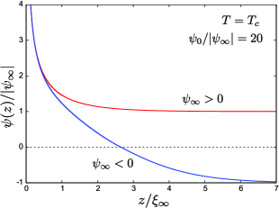
Figure 1: (Color online) Normalized order parameter $\psi(z)/|\psi_{\infty}|$ vs $z/\xi_{\infty}$ at $T=T_{c}$ in the semi-infinite case at $\psi_{0}=20|\psi_{\infty}|$ for positive and negative small $\psi_{\infty}$. The decay is algebraic for small $z$ as in Eq.(2.15) and is eventually exponential as in Eq.(2.18). For $\psi_{\infty}<0$, the approach to $\psi_{\infty}$ is slow and the adsorption is large as in Eq.(2.20).

II.3 Profiles between parallel plates

We assume that a mixture at $T=T_{c}$ is inserted between parallel plates separated by $D$. The plate area $S$ is assumed to be much larger than $D^{2}$ such that the edge effect is negligible. The fluid is in contact with a large reservoir containing the same binary mixture in equilibrium. In the reservoir, the mean order parameter is $\psi_{\infty}$ and the chemical potential is $\mu_{\infty}$ in Eq.(2.10). Then we minimize the excess grand potential (per unit area),

$$\Omega=\int_{0}^{D}dz[f_{\rm loc}-f_{\infty}-\mu_{\infty}(\psi-\psi_{\infty})]$$ (2.20)

The fluid is in the region $0<z<D$. At the walls $z=0$ and $D$, we assume the symmetric boundary conditions,

$$\psi(0)=\psi_{0},\quad\psi(D)=\psi_{0},$$ (2.21)

where $\psi_{0}>0$. Here Eq.(2.11) still holds, leading to

$$C(\psi)|d\psi/dz|^{2}=2\omega,$$ (2.22)

where $\omega$ is the excess grand potential density for a film,

$$\omega = f(\psi)-f_{m}-\mu_{\infty}(\psi-\psi_{m})$$ (2.23)

$$= \omega_{s}+f_{m}-f_{\infty}-\mu_{\infty}(\psi_{m}-\psi_{\infty})$$

Hereafter, $\psi_{m}=\psi(D/2)$ is the order parameter at the midpoint $z=D/2$ and $f_{m}=f(\psi_{m})$. From Eq.(2.13) $\omega-\omega_{s}$ is simply a constant. We require $d\psi/dz=0$ at $z=D/2$ or $\omega=0$ at $\psi=\psi_{m}$ because of the symmetric boundary conditions in Eq.(2.22). In the region $0<z<D/2$, $\psi=\psi(z)$ is obtained from

$$D/2-z=\int_{\psi_{m}}^{\psi}d\psi\sqrt{C(\psi)/2\omega(\psi)},$$ (2.24)

where $\omega=\omega(\psi)$ is treated as a function of $\psi$. As $z\to 0$, the plate separation distance $D$ is expressed as

$$D=\int_{\psi_{m}}^{\psi_{0}}d\psi\sqrt{2C(\psi)/\omega(\psi)},$$ (2.25)

which determines $\psi_{m}$ for each $D$, indicating the following. (i) In the integral of Eq.(2.26), we may push the upper bound $\psi_{0}$ to infinity for large $\psi_{0}$ since $1/\sqrt{\omega}\sim\psi^{-(1+\delta)/2}$ for large $\psi$. Thus $\psi_{m}$ becomes independent of $\psi_{0}$ as $\psi_{0}\to\infty$. (ii) For a thick film with $D\gtrsim\xi_{\infty}$, $\psi_{m}$ should approach $\psi_{\infty}$, where $\xi_{\infty}$ is the correlation length in Eq.(2.19). In the integrand of Eq.(2.26), we expand $\omega$ in powers of $\varphi\equiv\psi-\psi_{m}$ as

$$\omega = (\mu_{m}-\mu_{\infty})\varphi+f^{\prime\prime}(\psi_{m})\varphi^{2}/2+\cdots,$$ (2.26)

$$\cong f^{\prime\prime}(\psi_{m})[(\psi_{m}-\psi_{\infty})\varphi+\varphi^{2}/2],$$

where $\mu_{m}=\mu(\psi_{m})$. The second line follows for $\psi_{m}\cong\psi_{\infty}$. Using $\xi_{\infty}=[C(\psi_{\infty})/f^{\prime\prime}(\psi_{\infty})]^{1/2}$, we perform the integral in Eq.(2.26) as $2\xi_{\infty}\ln[\psi_{\infty}/(\psi_{m}-\psi_{\infty})]$ for $\psi_{\infty}\neq 0$. Thus, for $D\gtrsim\xi_{\infty}$, $\psi_{m}$ approaches $\psi_{\infty}$ as

$$\psi_{m}-\psi_{\infty}\sim\psi_{\infty}\exp({-D/2\xi_{\infty}}).$$ (2.27)

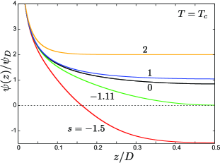
Figure 2: (Color online) Normalized order parameter $\psi(z)/\psi_{D}$ vs $z/D$ at $T=T_{c}$ in a film in the half region $0<z<D/2$ for $s=\psi_{\infty}/\psi_{D}=2,1,0,-1.11$, and -1.5 from above with $\psi_{0}=20\psi_{D}$ in the symmetric boundary conditions, where $\psi_{D}$ is defined by Eq.(2.9). The decay is algebraic for small $z$ as in Eq.(2.15).

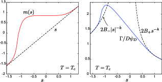
Figure 3: (Color online) Left: $m=\psi_{m}/\psi_{D}$ vs $s=\psi_{\infty}/\psi_{D}$ for a film at $T=T_{c}$ in the limit $\psi_{0}\to\infty$, where $\psi_{m}$ is the midpoint value, $\psi_{\infty}$ is the reservoir value, and $\psi_{D}\propto D^{-\beta/\nu}$. Here $m$ stays at $0.8$ in the weak response region ($-0.9\lesssim s\lesssim 0.7$), changes steeply in the catastrophic region ($-1.2\lesssim s\lesssim-0.9$), and tends to $s$ in the strong reservoir region ($|s|\gtrsim 1.1$). Right: Normalized adsorption $\Gamma/D\psi_{D}$ vs $s$ at $T=T_{c}$. It approaches $2B_{+}s^{-k}$ for $s\gtrsim 1$ and $2B_{-}|s|^{-k}$ for $s\lesssim-1$ (dotted lines) with $k=\nu/\beta-1$ from Eq.(2.20). The lines of $\Gamma/D\psi_{D}$ and $2B_{-}|s|^{-k}$ crosses at $s=-0.90$, where the Casimir amplitude $\Delta(s)$ is maximized from Eq.(2.52).

In the limit $\psi_{0}\to\infty$, the profile $\psi(z)$ is scaled in terms of a scaling function $\Psi(u,s)$ as

$$\psi(z)=\psi_{D}\Psi(z/D,\psi_{\infty}/\psi_{D}).$$ (2.28)

Hereafter, we set

$$s = \psi_{\infty}/\psi_{D},$$ (2.29)

$$m = \psi_{m}/\psi_{D}=\Psi(0.5,s),$$ (2.30)

which are the normalized order parameter in the reservoir and that at the midpoint, respectively. In Fig.2, for $\psi_{0}/\psi_{D}=20$, we plot $\psi(z)/\psi_{D}$ vs $z/D$ for five values of $s$. These profiles represent $\Psi(z/D,s)$ slightly away from the wall or for $z\gg\ell_{0}$. For $s=2$ and $-1.5$, we find $m\cong s$ (or $\psi_{m}\cong\psi_{\infty}$). However, the curves for $s=0$ and $s=1$ are very close, while that for $s=-1.11$ tends to 0 at the midpoint.

II.4 Weak response and catastrophic behaviors

In the left panel of Fig.3, we show $m$ vs $s$ determined by Eq.(2.26) in the limit $\psi_{0}\to\infty$. The slope of the curve $dm/ds$ is written as

$$\frac{dm}{ds}={\bigg{(}}\frac{\partial{\psi_{m}}}{\partial{\psi_{\infty}}}{\bigg{)}}_{D}=\frac{\chi_{m}}{\chi_{\infty}},$$ (2.31)

which is equal to the ratio of the two susceptibilities $\chi_{m}=k_{B}T_{c}\partial\psi_{m}/\partial\mu_{\infty}$ at the midpoint and $\chi_{\infty}=k_{B}T_{c}\partial\psi_{\infty}/\partial\mu_{\infty}$ in the reservoir Nakanishi-mean . Here, because of the large size of the critical exponent $\delta=4.815$, there are distinctly different three regions of $s$: (i) For $-0.9\lesssim s\lesssim 0.7$, $m$ is nearly a constant about 0.8 with $dm/ds\sim 0.1$. Here $m$ little changes with a change in $s$. The response of $\psi$ in the film to a change in $\psi_{\infty}$ is weak. (ii) For $-1.2\lesssim s\lesssim-0.9$, we have $dm/ds\sim 5\sim\delta$. In this catastrophic region, $m$ changes steeply between the base curve $m=s$ and 0.8. The width of this region is of order $1/\delta$ and is narrow. (iii) In the regions $s\gtrsim 1$ and $s\lesssim-1.3$, Eq.(2.28) gives

$$m-s\sim\exp[{-\sqrt{\delta(\delta+1)/2}|s|^{\nu/\beta}}].$$ (2.32)

That is, $\psi_{m}\cong\psi_{\infty}$ and the reservoir inflence is strong.

The excess adsorption $\Gamma=\int_{0}^{D}dz(\psi-\psi_{\infty})$ in the film with respect to the reservoir is expressed as

$$\Gamma=\int_{\psi_{m}}^{\psi_{0}}d\psi(\psi-\psi_{\infty})\sqrt{{2C(\psi)}/{\omega(\psi)}}$$ (2.33)

Again we may push the upper bound of the integral to infinity for large $\psi_{0}$; then, $\Gamma/D\psi_{D}$ becomes a universal function of $s$. At $T=T_{c}$, Eq.(2.20) indicates that $\Gamma\to 2\Gamma_{{\rm sem}\pm}=2D\psi_{D}B_{\pm}|s|^{1-\nu/\beta}$ for $D\gtrsim\xi_{\infty}$ or for $|s|\gtrsim 1$. It is convenient to introduce a scaling function $\Gamma^{*}(s)$ by

$$\Gamma=2\Gamma_{{\rm sem}\pm}+D\psi_{D}\Gamma^{*}.$$ (2.34)

In the right panel of Fig.3, we show $\Gamma/D\psi_{D}$ vs $s$ in the limit $\psi_{0}\to\infty$. In the weak response region, $-0.9\lesssim s\lesssim 0.7$, we have $\Gamma/D\psi_{D}\sim 0.5-s$. Thus $\Gamma/D\psi_{D}$ increases with decreasing $s$, exhibiting a peak at the border of the weak response and catastrophic regions. In fact, its maximum is 2.29 at $s=-0.94$. In the strong reservoir region, it approaches $2B_{\pm}|s|^{-k}$ with $k=\nu/\beta-1$ (see the dotted lines in the right panel of Fig.3).

II.5 Casimir term in the force density

Using Eq.(2.23), the excess grand potential $\Omega$ in Eq.(2.21) is expressed in terms of $\omega=\omega(\psi)$ as

$$\Omega = D[f_{m}-f_{\infty}-\mu_{\infty}(\psi_{m}-\psi_{\infty})]$$ (2.35)

$$+2\int_{\psi_{m}}^{\psi_{0}}d\psi\sqrt{2C(\psi)\omega(\psi)}.$$

In the right hand side, the first term arises due to the reservoir. In the second term, the gradient contribution gives rise to the factor 2. Let us calculate the derivative $\partial\Omega/\partial D$ at fixed $\psi_{0}$ and $\psi_{\infty}$, treating $\psi_{m}$ as a function of $D$. The derivative of the second term is $D(\mu_{\infty}-\mu_{m})\partial\psi_{m}/\partial D$ from Eq.(2.26), where $\mu_{m}=f^{\prime}(\psi_{m})$. We then find a simple expression,

$$\frac{\partial\Omega}{\partial D}=f_{m}-f_{\infty}-\mu_{\infty}(\psi_{m}-\psi_{\infty}).$$ (2.36)

The Casimir amplitude of the force density ${\cal A}=({\partial\Omega}/{\partial D}){D^{d}}/{k_{B}T_{c}}$ is expressed as

$${\cal A}=\frac{D^{d}}{k_{B}T_{c}}\bigg{[}f_{m}-f_{\infty}-\mu_{\infty}(\psi_{m}-\psi_{\infty})\bigg{]}.$$ (2.37)

Note that the osmotic pressure $\Pi$ is the force density per unit area exerted by the fluid to the walls. See Appendix A for more discussions. Thus we find Tsori

$$\Pi=-\frac{\partial\Omega}{\partial D}=-k_{B}T_{c}{\cal A}/D^{d}.$$ (2.38)

From the second line of Eq.(2.24) we also notice the relation $\omega(\psi)-\omega_{s}(\psi)=-\partial\Omega/\partial D$. Equations (2.36)-(2.39) hold even for $T\neq T_{c}$ in our theory in the next section.

At $T=T_{c}$, use of Eqs.(2.3), (2.8), and (2.9) gives

$$\frac{1}{A_{c}}{\cal A}(s)=\delta|s|^{1+\delta}+|{m}|^{1+\delta}-(1+\delta)|s|^{1+\delta}\frac{m}{s}.$$ (2.39)

in terms of $s$ in Eq.(2.30) and $m$ in Eq.(2.31). We can see that ${\cal A}={\cal A}(s)$ is a universal function of $s$ as $\psi_{0}\to\infty$. In Eq.(2.26) we set $\psi=\psi_{D}q$ to obtain

$$\int_{m}^{\infty}dqq^{-\eta\nu/2\beta}/\sqrt{{{\hat{\omega}}}(q,s,m)}=1,$$ (2.40)

where $\hat{\omega}=\omega/B_{0}\psi_{D}^{1+\delta}$ depends on $q$, $s$, and $m$ as

$$\hat{\omega}=|q|^{1+\delta}-|m|^{1+\delta}-(1+\delta)|s|^{\delta-1}s(q-m).$$ (2.41)

We seek $m=m(s)$ for each $s$ from Eq.(2.41) (as given in the left panel of Fig.3). In particular, for $|s|\gg 1$, we have $\psi_{m}\to\psi_{\infty}$ and $\partial\Omega/\partial D\propto(\psi_{m}-\psi_{\infty})^{2}$ from Eq.(2.37). From Eq.(2.28) ${\cal A}(s)$ decays for $|s|\gtrsim 1$ as

$${\cal A}(s)\sim e^{-D/\xi_{\infty}}\sim\exp[{-\sqrt{2\delta(\delta+1)}|s|^{\nu/\beta}}].$$ (2.42)

We calculate ${\cal A}(s)$ for two special cases. (i) First, for $s=0$, the reservoir is at the criticality. Here, $m>0$, so setting $v=q/m$ in Eq.(2.41) gives $m^{\nu/\beta}=I_{0}$ with

$$I_{0}=\int_{1}^{\infty}dv{v^{-\eta\nu/2\beta}}/{\sqrt{v^{1+\delta}-1}}.$$ (2.43)

where $I_{0}=0.719$ for $d=3$. Since $\partial\Omega/\partial D=f(\psi_{m})$, we obtain the critical-point value ${\cal A}_{\rm cri}={\cal A}(0)$ in the form,

$${\cal A}_{\rm cri}=I_{0}^{d}A_{c},$$ (2.44)

where $A_{c}$ is given by Eq.(2.8) and will be estimated below Eq.(3.16). Essentially the same calculation was originally due to Borjan and Upton Upton . (ii) Second, we assume $\psi_{m}=0$, which is attained for $\psi_{\infty}<0$ or for $s<0$. See the corresponding curve of $s=-1.11$ in Fig.2. From Eq.(2.41) we obtain $|s|^{\nu/\beta}=J_{0}$ with

$$J_{0}=\int_{0}^{\infty}dvv^{-\eta\nu/2\beta}/\sqrt{v^{1+\delta}+(1+\delta)v},$$ (2.45)

where $J_{0}=1.195$ at $d=3$ numerically, leading to $s=-J_{0}^{\beta/\nu}=-1.1170$. From Eqs.(2.40) and (2.45) we find

$${\cal A}(-1.1170)=J_{0}^{d}A_{c}\delta={\cal A}_{\rm cri}(J_{0}/I_{0})^{d}\delta,$$ (2.46)

Thus ${\cal A}(-1.1170)/{\cal A}_{\rm cri}=24.45$ for $d=3$.

In Fig.4, we display ${\cal A}(s)/{\cal A}_{\rm cri}$ for $d=3$ calculated from Eqs.(2.40) and (2.41). Its maximum is 24.45 at $s=-1.1170$, where $\psi_{m}\cong 0$. To be precise, the curve exhibits a small cusp due to the weak $\psi$-dependence of $C(\psi)$. Similar enhancement of $\cal A$ was found at off-critical compositions by Maciołek et al Evans-Anna for two-diemnsional Ising films and by Schlesener et al. JSP in the mean-field theory at $T=T_{c}$. In the next section, the origin of this peak will be ascribed to the fact that the peak point on the line $T=T_{c}$ is very close to a capillary-condensation critical point in the region $T<T_{c}$ (see Figs.9 and 12).

Mathematically, the peak of ${\cal A}(s)$ at $T=T_{c}$ stems from the presence of the weak response and catastrophic regions, for which see the explanation of the right panel of Fig.3. Here we calculate $d{\cal A}(s)/ds$ from Eq.(2.40) as

$$\frac{1}{a|s|^{\delta-1}}\frac{d{\cal A}}{ds}=\bigg{(}{\bigg{|}\frac{m}{s}\bigg{|}^{\delta-1}}\frac{m}{\delta}-\frac{s}{\delta}\bigg{)}\frac{dm}{ds}-m+s,$$ (2.47)

where $a=A_{c}(1+\delta)\delta\sim 28A_{c}\sim 40$. In the weak response region, we may neglect the first term in the right hand side to obtain $d{\cal A}/ds\cong-a|s|^{\delta-1}(m-s)<0$, which is nearly zero for $s\gtrsim-0.5$ and grows abruptly for $s\lesssim-0.5$. In the catastrophic region, $dm/ds$ is of order $\delta$ such that $d{\cal A}/ds$ changes its sign, leading to a maximum of $\cal A$.

II.6 Casimir term in the grand potential

For binary mixtures, the de Gennes-Fisher scaling form Fisher for the grand potential reads

$$\Omega=\Omega_{\infty}-k_{B}TD^{-(d-1)}{\Delta},$$ (2.48)

where $\Omega_{\infty}=\lim_{D\to\infty}\Omega$ is the large-separation limit. The $\Delta$ is a function of $s$ in Eq.(2.30) (and a scaled reduced temperature in the next section). This form may be inferred from the boundary behavior of $f_{\rm loc}$ in Eq.(2.17). Next, we differentiate Eq.(2.36) with respect to $\mu_{\infty}$ (or $\psi_{\infty}$) at fixed $D$ and $\psi_{0}$. Following the procedure used in deriving Eq.(2.37), we obtain the Gibbs adsorption formula Evans-Marconi ,

$$\frac{\partial\Omega}{\partial\mu_{\infty}}=\frac{\chi_{\infty}}{k_{B}T_{c}}\frac{\partial\Omega}{\partial\psi_{\infty}}=-\Gamma,$$ (2.49)

where $\Gamma$ is the excess adsorption in Eq.(2.34) and $\chi_{\infty}=k_{B}T_{c}/f^{\prime\prime}(\psi_{\infty})$. If the Fisher-de Gennes form (2.49) is substituted into Eq.(2.50), the above relation yields

$$\frac{\partial\Delta}{\partial s}=R_{\infty}\Gamma^{*}$$ (2.50)

where $\Gamma^{*}$ is defined by Eq.(2.35) and $R_{\infty}$ is the following dimensionless combination representing the scaled inverse susceptibility in the reservoir,

$$R_{\infty}={D^{d}}\psi_{D}^{2}/\chi_{\infty}.$$ (2.51)

At $T=T_{c}$, we obtain $R_{\infty}=A_{c}\delta(\delta+1)|s|^{\delta-1}$, which has already appeared in Eq.(2.48) as $a|s|^{\delta-1}$. In our theory in the next section, Eqs. (2.49)-(2.52) will remain valid even for $T\neq T_{c}$.

At $T=T_{c}$, direct differentiation of $\Omega$ in Eq.(2.49) with respect to $D$ also yields a relation between ${\cal A}(s)$ and $\Delta(s)$,

$${\cal A}(s)=(d-1){\Delta}(s)-\frac{\beta s}{\nu}\frac{\partial}{\partial s}{\Delta}(s).$$ (2.52)

Elimination of $\partial\Delta/\partial s$ from Eqs.(2.51) and (2.53) yields

$$\Delta(s)=\frac{{\cal A}(s)}{d-1}+\frac{dA_{c}}{d-1}\delta|s|^{\delta-1}s\Gamma^{*}(s).$$ (2.53)

Thus, as well as ${\cal A}$, $\Delta$ is proportional to the universal number $A_{c}$. The critical-point values of the amplitudes, written as $\Delta_{\rm cri}=\Delta(0)$ and ${\cal A}_{\rm cri}={\cal A}(0)$, are related as

$$\Delta_{\rm cri}={\cal A}_{\rm cri}/(d-1).$$ (2.54)

In Fig.4, we also plot ${\Delta}(s)/{\Delta}_{\rm cri}$ for $d=3$ numerically calculated from Eq.(2.54). Its peak height is $13.36$ at $s=-0.90$, which is about half of the height of ${\cal A}(s)/{\cal A}_{\rm cri}$. The differential equation (2.53) is excellently satisfied by ${\cal A}(s)$ and ${\Delta}(s)$ in Fig.4. From Eq.(2.51) the amplitude $\Delta(s)$ is maximized at a point where $\Gamma^{*}=0$. Indeed, in the right panel of Fig.3, the line of $\Gamma/D\psi_{D}$ vs $s$ and that of $2B_{-}|s|^{\nu/\beta-1}$ vs $s$ cross at $s=-0.90$, where $\Delta(s)$ is maximum in Fig.4.

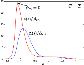
Figure 4: (Color online) Casimir amplitude ratios ${\cal{A}}(s)/{\cal{A}}_{\rm cri}$ for the force density and $\Delta(s)/\Delta_{\rm cri}$ for the grand potential vs $s=\psi_{\infty}/\psi_{D}$ at $T=T_{c}$ in the limit $\psi_{0}\to\infty$. These quantities are maximized at $s\sim-1$ upon the changeover between the weak response and catastrophic regions (see the text).

III Critical behavior for $T\neq T_{c}$

In this section, we now set up a local functional theory including the gradient free energy for nonvanishing reduced temperature,

$$\tau=T/T_{c}-1.$$ (3.1)

For binary mixtures, we suppose the upper critical solution temperature (UCST), while $\tau$ should be defined as $\tau=1-T/T_{c}$ for the lower critical solution temperature (LCST). Our model is similar to the linear parametric model by Schofield et al. Sc69 ; Hohenberg ; Wallace2 and the local functional model by Upton et al. Fisher-Upton ; Upton ; Upton1 ; Upton-ad . The latter is composed of the free energy of the linear parametric model and the gradient free energy. We use a simpler free energy accounting for the renormalization effect and the gradient free energy. Further, we define the free energy within the coexistence curve and make it satisfy the two-scale-factor universalityStauffer ; HAHS . Appendix B will give the relationship between our model and the linear parametric model.

The Casimir amplitudes ${\cal A}$ in Eq.(2.38) and ${\Delta}$ in Eq.(2.49) depend on $s=\psi_{\infty}/\psi_{D}$ in Eq.(2.30) and the scaled reduced temperature,

$$t=\tau(D/\xi_{0})^{1/\nu}.$$ (3.2)

where $\xi_{0}$ is a microscopic length ($\sim 3\rm{\AA}$) in the correlation length $\xi=\xi_{0}\tau^{-\nu}$ for $\tau>0$ at the critical composition. For example, $\xi/D$ is $0.24$ for $t=10$ and $0.056$ for $t=100$.

III.1 Model outside the coexistence curve

For $\tau<0$, two phases can coexist in the bulk. The coexistence curve is written as $\psi=\pm\psi_{\rm cx}$ with

$$\psi_{\rm cx}=b_{\rm cx}|\tau|^{\beta},$$ (3.3)

where $b_{\rm cx}$ is a constant. In this subsection, we present a local free energy density $f_{\rm loc}$ applicable outside the coexistence curve ($|\psi|\geq\psi_{\rm cx}$ if $\tau<0$). In the next subsection, we present its form within the coexistence curve.

As a generalization of the model in Eqs.(2.1)-(2.4) for $\tau=0$, we again use the usual form,

$$f_{\rm loc}=f+\frac{1}{2}k_{B}T_{c}C|\nabla\psi|^{2}.$$ (3.4)

The free energy density $f=f(\psi,\tau)$ is an even function of $\psi$ expressed as

$$f=k_{B}T_{c}\bigg{(}\frac{1}{2}r\psi^{2}+\frac{1}{4}u\psi^{4}\bigg{)}.$$ (3.5)

Here $r$, $u$, and $C$ are renormalized coefficients depending on $\psi$ and $\tau$. To account for the renormalization effect, we introduce a distance from the critical point $w$. In the critical region ($w\ll 1$), these coefficients depend on $w$ as

$$C = C_{1}w^{-\eta\nu},$$ (3.6)

$$r = C_{1}\xi_{0}^{-2}w^{\gamma-1}\tau,$$ (3.7)

$$u = C_{1}^{2}u^{*}\xi_{0}^{-\epsilon}w^{(\epsilon-2\eta)\nu},$$ (3.8)

where $C_{1}$ and $u^{*}$ are constants. For $\tau>0$ and $\psi=0$, we set $w=\tau$ to obtain $\xi^{2}=C/r$. For $\tau=0$, we should have $w^{2\beta}\propto\psi^{2}$. We thus determine $w$ as a function of $\tau$ and $\psi^{2}$ from

$$w=\tau+C_{2}w^{1-2\beta}\psi^{2},$$ (3.9)

where $C_{2}$ is a constant. Recall the mean-field expression $\chi^{-1}=r+3u\psi^{2}$ for the susceptibility $\chi$, which holds even for $r<0$. If we use Eqs.(3.6)-(3.8), we have $r+3u\psi^{2}=C_{1}\xi_{0}^{-2}w^{\gamma-1}[\tau+3C_{1}u^{*}\xi_{0}^{2-\epsilon}w^{1-2\beta}\psi^{2}]$ in our renormalized theory. Thus we may require

$$r+3u\psi^{2}=C_{1}\xi_{0}^{-2}w^{\gamma},$$ (3.10)

where we relate $C_{2}$ in Eq.(3.9) to $C_{1}$ as

$$C_{2}=3u^{*}C_{1}\xi_{0}^{2-\epsilon}.$$ (3.11)

See Fig.5 for $f$ and $w$ as functions of $\psi$ for fixed positive $\tau$. In the simplest case $\tau>0$ and $\psi=0$, we have $w=\tau$ and $w^{\nu}=\xi_{0}/\xi$ so that the concentration susceptibility $\chi(\tau,\psi)=k_{B}T_{c}(\partial\psi/\partial\mu)_{\tau}$ grows strongly with the exponent $\gamma$ as

$$\chi(\tau,0)=r=C_{1}^{-1}\xi_{0}^{2}\tau^{-\gamma}.$$ (3.12)

In the renormalization group theory Onukibook , Eqs.(3.6)-(3.9) follow if $\xi_{0}^{-1}w^{\nu}$ is the lower cut-off wave number of the renormalization. The coupling constant $u^{*}$ should be a universal fixed-point value. Its $\epsilon$ expansion reads

$$K_{d}u^{*}=\epsilon/9+\cdots,$$ (3.13)

where $K_{d}$ is the surface area of a unit sphere in $d$ dimensions divided by $(2\pi)^{d}$ (so $K_{4}=1/8\pi^{2}$ and $K_{3}=1/2\pi^{2}$). Retaining the small critical exponent $\eta\propto\epsilon^{2}$ and using the relations among the critical exponents, we may correctly describe the asymptotic scaling behavior, though the critical amplitude ratios are approximate. In addition, note that a constant term independent of $\psi$ has been omitted in the singular free energy density in Eq.(3.5), which yields the singular specific heatconstant .

For $\tau=0$, the Fisher-Au Yang model in Eq.(2.1) folows with $C_{0}$ and $B_{0}$ given by

$$C_{0}/k_{B}T_{c} = C_{1}C_{2}^{-\eta\nu/2\beta},$$ (3.14)

$$B_{0}/k_{B}T_{c} = u^{*}C_{1}^{2}C_{2}^{(\epsilon/2-\eta)\nu/\beta}\xi_{0}^{-\epsilon}/4.$$ (3.15)

Thus we have $B_{0}k_{B}T_{c}/C_{0}^{2}=u^{*}C_{2}^{\epsilon\nu/2\beta}/4\xi_{0}^{\epsilon}$ and $B_{0}/C_{0}=u^{*}C_{1}C_{2}^{\nu/\beta-1}\xi_{0}^{-\epsilon}/4=C_{2}^{\nu/\beta}/12\xi_{0}^{2}$. The universal number $A_{c}$ in Eq.(2.8) is calculated as

$$A_{c}=2^{d}6^{-\epsilon/2}/u^{*}.$$ (3.16)

As a rough estimate, we set $u^{*}=1/9K_{3}=2\pi^{2}/9$ for $d=3$ from Eq.(3.13). This leads to $A_{c}=(2^{3}/\sqrt{6})/u^{*}=1.49$. This value yields $\Delta_{\rm cri}={\cal A}_{\rm cri}/2=0.279$ from Eq.(2.45). For $d=3$, Krech Krech estimated $\Delta_{\rm cri}$ to be $0.326$ by a field-theoretical methods and $0.345$ by a Monte Carlo method, Borjan and Upton Upton obtained $\Delta_{\rm cri}=0.428$ by the local functional theory, and Vasilyev et al. Monte found ${\Delta}_{\rm cri}=0.442$ by a Monte Carlo method.

To make the following expressions for $f$ and $\mu$ simpler, we introduce the dimensionless ratio,

$$S=\tau/w,$$ (3.17)

in terms of which $\psi^{2}$ is expressed as

$$\psi^{2}=(1-S)w^{2\beta}/C_{2}.$$ (3.18)

Then $f$ and $\mu=(\partial f/\partial\psi)_{\tau}$ are expressed as

$$\frac{f}{k_{B}T_{c}}=\frac{w^{2-\alpha}}{36u^{*}\xi_{0}^{d}}(1+5S)(1-S),$$ (3.19)

$$\frac{\mu}{k_{B}T_{c}}=\frac{2-\alpha+4(1-\alpha)S+5\alpha S^{2}}{18u^{*}[2\beta+(1-2\beta)S]\xi_{0}^{d}}w^{\gamma}C_{2}\psi.$$ (3.20)

In Eq.(3.20), we have used the relation $({\partial w}/{\partial\psi})_{\tau}={2C_{2}w^{1-2\beta}\psi}/[{2\beta+(1-2\beta)S}]$. However, the susceptibility $\chi(\tau,\psi)=k_{B}T_{c}/(\partial\mu/\partial\psi)$ is somewhat complicated sus . It can be simply calculated for $\mu=0$ as in Eq.(3.12) for $\tau>0$ and as in Eq.(3.24) below for $\tau<0$.

We now seek the coexistence curve (3.3) by setting $\mu=0$ with $\tau<0$. From Eq.(3.20) it follows the quadratic equation $2-\alpha+4(1-\alpha)S+5\alpha S^{2}=0$ of $S$, which is solved to give $S=-1/\sigma$ or

$$w=\sigma|\tau|.$$ (3.21)

The coefficient $\sigma$ is expressed in terms of $\alpha$ as

$$\sigma=2-9\alpha/[2+\sqrt{4-18\alpha+9\alpha^{2}}],$$ (3.22)

which is equal to 1.714 for $d=3$. If we substitute Eq.(3.21) into Eq.(3.9), the coefficient $b_{\rm cx}$ in Eq.(3.2) is calculated as

$$b_{\rm cx}=C_{2}^{-1/2}(1+\sigma)^{1/2}\sigma^{\beta-1/2},$$ (3.23)

leading to $C_{2}=(1+\sigma)\sigma^{2\beta-1}/b_{\rm cx}^{2}$. Since $b_{\rm cx}$ is experimentally measurable, there remains no arbitrary parameter with Eqs.(3.11) and (3.23). The susceptibility $\chi$ on the coexistence curve is expressed as

$$\chi(-|\tau|,\psi_{\rm cx})=\frac{3\sigma}{2\zeta(1+\sigma)}C_{1}^{-1}\xi_{0}^{2}|\sigma\tau|^{-\gamma}.$$ (3.24)

In the denominator of this relation, we introduce

$$\zeta=\frac{2(1-\alpha)\sigma-5\alpha}{(2\beta\sigma-1+2\beta)^{2}},$$ (3.25)

which is equal to 4.28 for $d=3$. The ratio of the susceptibility for $\tau>0$ and $\psi=0$ and that on the coexistence curve at the same $|\tau|$ is written as

$$R_{\chi}=\frac{\chi(|\tau|,0)}{\chi(-|\tau|,\psi_{\infty})}=\frac{2}{3}\zeta(1+\sigma)\sigma^{\gamma-1},$$ (3.26)

which is 8.82 for $d=3$. Note that the $\epsilon$ expansion gives $R_{\chi}=(2+\epsilon)2^{\epsilon/6}+\cdots$ and its reliable estimate is 4.9 Nicoll ; Liu1 ; Onukibook . We also write the correlation length on the coexistence curve as $\xi=(C/f^{\prime\prime})^{1/2}=\xi_{0}^{\prime}|\tau|^{-\nu}$, where $\xi_{0}^{\prime}$ is another microscopic length. The ratio of the two microscopic lengths $\xi_{0}$ and $\xi_{0}^{\prime}$ is written as

$$\xi_{0}/\xi_{0}^{\prime}=[2\zeta(1+\sigma)\sigma^{2\nu-1}/3]^{1/2},$$ (3.27)

which gives $\xi_{0}/\xi_{0}^{\prime}=2.99$ for $d=3$. Note that the $\epsilon$ expansion result is $\xi_{0}/\xi_{0}^{\prime}=2^{\nu}(1+5\epsilon/24+\cdots)$ and its reliable estimate is 1.9 for $d=3$ Nicoll ; Liu1 ; Onukibook . We recognize that the correlation length $\xi$ and the susceptibility $\chi$ on the coexistence curve are considerably underestimated in our theory (mainly due to a factor $Z(\theta)$ in Eq.(B13) in Appendix B).

Finally, let us consider the characteristic order parameter of a film $\psi_{D}$ defined in Eq.(2.9). From the sentence below Eq.(3.15) it is written as

$$\psi_{D} = C_{2}^{-1/2}(\sqrt{24}\xi_{0}/D)^{\beta/\nu}$$ (3.28)

$$= 1.47b_{\rm cx}(\xi_{0}/D)^{\beta/\nu}$$

where $b_{\rm cx}$ is given by Eq.(3.23). Equation (3.18) gives an expression for $\psi$ valid outside the coexistence curve,

$$|\psi|/\psi_{D}=24^{-\beta/2\nu}(1-S)^{1/2}|S|^{-\beta}|t|^{\beta}.$$ (3.29)

On the coexistence curve, this expression becomes

$${\psi_{\rm cx}}/{\psi_{D}}=24^{-\beta/2\nu}(1+\sigma^{-1})^{1/2}\sigma^{\beta}|t|^{\beta},$$ (3.30)

which is equal to $0.66|t|^{\beta}$ in our theory.

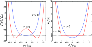
Figure 5: (Color online) Normalized singular free energy density $f(\psi)/f_{\rm cri}$ (left) and normalized distance from the criticality $w/|\tau|=1/|S|$ (right) vs $\psi/\psi_{\rm cx}$, where $f_{\rm cri}=k_{B}T_{c}|\tau|^{2-\alpha}/u^{*}\xi_{0}^{d}$ and $\psi_{\rm cx}=b_{\rm cx}|\tau|^{\beta}$ (both for $\tau>0$ and $\tau<0$). The upper (lower) curves correspond to those for $\tau>0$ ($\tau<0$). For $\tau<0$, $w$ is independent of $\psi$ within the coexistence curve $|\psi|/\psi_{\rm cx}<1$ in our model.

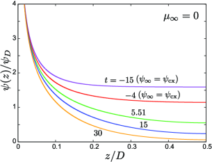
Figure 6: (Color online) Normalized order parameter $\psi(z)/\psi_{D}$ vs $z/D$ for $\mu_{\infty}=0$ in a film in the half region $0<z<D/2$ for $t=30,15,5.51$, -4, and -15 from below with $\psi_{0}=20\psi_{D}$ in the symmetric boundary conditions. Here $\psi_{\infty}=0$ for $t>0$ and $\psi_{\infty}=\psi_{\rm cx}$ for $t<0$. The decay is algebraic for small $z$ as in Eq.(2.15).

III.2 Model including the coexistence curve interior

For $\tau<0$, we need to define a local free energy density $f$ inside the coexistence curve $|\psi|<\psi_{\rm cx}$, where the fluid is metastable or unstable in the bulk. Notice that $\psi(z)$ changes from $-\psi_{\rm cx}$ to $\psi_{\rm cx}$ in the interface region in two-phase coexistence. Thus, to calculate the surface tension in the Ginzburg-Landau scheme, we need $f(\psi)$ in the region $|\psi|\leq\psi_{\rm cx}$ for $\tau<0$. Since the linear parametric model is not well defined within the coexistence curve, Fisher et al. Fisher-Upton proposed its generalized form applicable even within the coexistence curve to obtain analytically continued van der Waals loops. We propose a much simpler model, though the derivatives $\partial^{\ell}f/\partial\psi^{\ell}$ in our model are continuous only up to $\ell=2$ on the coexistence curve.

Within the coexistence curve, we assume a $\psi^{4}$ theory including the gradient free energy. Since $\mu=\partial f/\partial\psi$ vanishes on the coexistence curve, $f$ is of the form,

$${f}={f_{\rm cx}}+\frac{1}{4}{k_{B}T_{c}}B_{\rm cx}(\psi^{2}-\psi_{\rm cx}^{2})^{2},$$ (3.31)

where ${f_{\rm cx}}$ is the value of $f$ on the coexistence curve. From Eq.(3.19) it is written as

$$f_{\rm cx}={k_{B}T_{c}}(\sigma-5)(1+\sigma)|\tau|^{2-\alpha}/{36u^{*}\xi_{0}^{d}\sigma^{\alpha}}.$$ (3.32)

We determine the coefficient ${B_{\rm cx}}$ requiring the continuity of the second derivative $f^{\prime\prime}=k_{B}T_{c}/\chi$. Then we obtain $2B_{\rm cx}\psi_{\rm cx}^{2}=1/\chi$, where $\chi$ is given by Eq.(3.24). Some calculations give a simple result,

$$B_{\rm cx}=\zeta u_{\rm cx},$$ (3.33)

where $\zeta$ is given by Eq.(3.25) and $u_{\rm cx}$ is the value of $u$ in Eq.(3.8) on the coexistence curve written as

$$u_{\rm cx}=C_{1}^{2}u^{*}\xi_{0}^{-\epsilon}|\sigma\tau|^{(\epsilon-2\eta)\nu}.$$ (3.34)

It follows the relation $f_{\rm cx}={k_{B}T_{c}}u_{\rm cx}\psi_{\rm cx}^{4}({\sigma-5})/{4(1+\sigma)}$. The coefficient of the gradient term is replaced by its value $C_{\rm cx}$ on the coexistence curve:

$$C_{\rm cx}=C_{1}|\sigma\tau|^{-\eta\nu},$$ (3.35)

Then the susceptibility $\chi$ and the correlation length $\xi$ are continuous across the coexistence curve. In this model, the renormalization effect inside the coexistence curve is the same as that on the coexistence curve at the same $\tau$. See Fig.5 for $f$ and $w$ vs $\psi$ for fixed negative $\tau$.

The surface tension $\sigma_{s}$ is given by the classical formula $\sigma_{s}=2k_{B}T_{c}C_{\rm cx}\psi_{\rm cx}^{2}/3\xi$ in the $\phi^{4}$ theory Onukibook . It is proportional to $\xi^{-d+1}$ with $\xi=\xi_{0}^{\prime}|\tau|^{-\nu}$. Some calculations give the universal number,

$$A_{s} = \sigma_{s}\xi^{d-1}/k_{B}T_{c}$$ (3.36)

$$= [2\zeta(1+\sigma^{-1})/3]^{\epsilon/2}/3\zeta u^{*}.$$

Using Eq.(3.25), we have $A_{s}=0.165/u^{*}$. Further, if we set $u^{*}=2\pi^{2}/9$, we obtain $A_{s}=0.075$. Note that $A_{\sigma}$ is known to be about 0.09 for Ising-like systems Moldover .

III.3 Casimir amplitudes for $T\neq T_{c}$

From Eq.(2.38) we can readily calculate ${\cal A}(t,s)$ numerically as a function of $s$ and $t$. However, to calculate $\Delta(t,s)$, we cannot use Eq.(2.54) for $t\neq 0$ and need to devise another expression. To this end, we write the second term in the right hand of Eq.(2.36) as

$$J=\Omega-D\frac{\partial\Omega}{\partial D}=2\int_{\psi_{m}}^{\psi_{0}}d\psi\sqrt{2C(\psi)\omega(\psi)},$$ (3.37)

where $\omega(\psi)$ is defined by Eq.(2.24) with $f$ being given by Eqs.(3.5) and (3.31). In the limit $D\to\infty$, we have $J\to\Omega_{\infty}$, where $\Omega_{\infty}$ is the large-separation limit:

$$\Omega_{\infty}=2\int_{\psi_{\infty}}^{\psi_{0}}d\psi\sqrt{2C(\psi)\omega_{s}(\psi)}.$$ (3.38)

Here, the lower bound of the integration is $\psi_{\infty}$ and $\omega_{s}(\psi)$ is the grand potential density for the semi-infinite case in the form of Eq.(2.13). Dividing the integration region in Eq.(3.38) into $[\psi_{m},\psi_{0}]$ and $[\psi_{\infty},\psi_{m}]$, we find

$$J-\Omega_{\infty} = 2\int_{\psi_{m}}^{\psi_{0}}d\psi{\sqrt{2C(\psi)}}[\sqrt{\omega(\psi)}-\sqrt{\omega_{s}(\psi)}]$$ (3.39)

$$-2\int_{\psi_{\infty}}^{\psi_{m}}d\psi\sqrt{2C(\psi)\omega_{s}(\psi)}.$$

In the first integral, we may push the upper bound $\psi_{0}$ to infinity, since the integrand tends to zero rapidly for large $\psi$ from $\sqrt{\omega}-\sqrt{\omega_{s}}=-(\partial\Omega/\partial D)/[\sqrt{\omega}+\sqrt{\omega_{s}}]$ (see the sentence below Eq.(2.39)). From Eqs.(2.37) and (2.49) we obtain

$$\Delta=-{\cal A}-\frac{D^{d-1}}{k_{B}T_{c}}(J-\Omega_{\infty}).$$ (3.40)

With this expression, we can calculate $\Delta(s,t)$ numerically, We confirm that it is a function of $s$ and $t$ only.

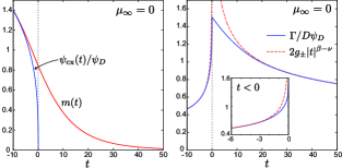
Figure 7: (Color online) Left: Normalized midpoint order parameter $m(t)=\psi_{m}(t)/\psi_{D}$ vs $t=\tau(D/\xi_{0})^{1/\nu}$ for a film with thickness $D$, where $s=0$ for $\tau>0$ and $s=\psi_{\rm cx}/\psi_{\rm cx}$ for $\tau<0$ ($\mu_{\infty}=0$). The coexistence curve $\psi_{cx}(t)/\psi_{D}$ vs $t$ in Eq.(3.3) is also shown in the region $t<0$. Right: Normalized excess adsorption $\Gamma/D\psi_{D}$ vs $t$ for $\mu_{\infty}=0$, whose maximum is $1.51$ at $t=0$. It tends to $2g_{\pm}|t|^{\beta-\nu}$ for $t\gtrsim 10$ and for $t\lesssim-1$ with $g_{+}=1.245$ and $g_{-}=0.471$, respectively (see Eq.(3.45)).

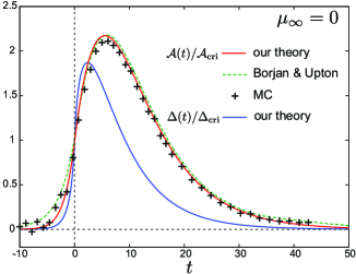
Figure 8: (Color online) ${\cal{A}}(t)/{\cal{A}}_{\rm cri}$ vs $t=\tau(D/\xi_{0})^{1/\nu}$ along the critical path $\mu_{\infty}=0$ from our theory (red bold line) and from Borjan and Upton’s theory Upton1 (blue broken line), which are in good agreement with the Monte Carlo data ($+$) Monte . Also plotted is $\Delta(t)/\Delta_{\rm cri}$ vs $t$ from our theory on the critical path.

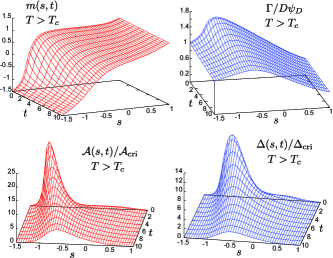
Figure 9: (Color online) Normalized midpoint order parameter $m(s,t)=\psi_{m}/\psi_{D}$ (top left), normalized excess adsorption $\Gamma/\psi_{D}D$ (top right), ${\cal{A}}(s,t)/{\cal{A}}_{\rm cri}$ (bottom left), and $\Delta(s,t)/\Delta_{\rm cri}$ (bottom right) for $t>0$ in the $s$-$t$ plane. The latter three quantities are peaked for $s\sim-1$. The amplitudes ${\cal{A}}(s,t)$ and $\Delta(s,t)$ are very small for $t\gg 1$ and $|s|\gg 1$.

In our theory, Eqs.(2.36)-(2.39) and Eqs.(2.49)-(2.51) remain valid even for $t\neq 0$. We now treat $m$, ${\cal A}$, $\Delta$, and $\Gamma^{*}$ as functions of $s$ and $t$, so $\partial(\cdots)/\partial s=(\partial(\cdots)/\partial s)_{t}$ and $\partial(\cdots)/\partial t=(\partial(\cdots)/\partial t)_{s}$. From Eq.(2.38) we obtain the generalized form of Eq.(2.48) as

$$\frac{1}{R_{\infty}}\frac{\partial\cal A}{\partial s}=\frac{\mu_{m}-\mu_{\infty}}{\psi_{D}k_{B}T_{c}}{\chi_{\infty}}\frac{\partial m}{\partial s}-(m-s).$$ (3.41)

Here, $R_{\infty}$ is a function of $s$ and $t$ defined by Eq.(2.52) (see Fig.16 for its overall behavior in the $s$-$t$ plane). Although redundant, we again write Eq.(2.51) as

$$\frac{1}{R_{\infty}}\frac{\partial\Delta}{\partial s}=\Gamma^{*},$$ (3.42)

which follows from the Gibbs adsorption relation. Here, $\Gamma^{*}$ is defined by Eq.(2.35), where the excess adsorption in the semi-infinite case $\Gamma_{{\rm sem}\pm}$ should be calculated for each given $\psi_{\infty}$ and $\tau$. In addition, differentiation of Eq.(2.49) with respect to $D$ yields the generalization of Eq.(2.53):

$${\cal A}=(d-1){\Delta}-\frac{\beta s}{\nu}\frac{\partial\Delta}{\partial s}-\frac{t}{\nu}\frac{\partial\Delta}{\partial t}.$$ (3.43)

III.4 Results for $T>T_{c}$

We first give some analysis along the critical path $\mu_{\infty}=0$, where $\psi_{\infty}=0$ for $t>0$ and $\psi_{\infty}=\psi_{\rm cx}>0$ for $t<0$. Numerical and experimental studies on the critical adsorption and the Casimir amplitudes have mostly been along this path in the literature Ha ; Monte ; Krech ; Lawreview ; adDietrich ; Upton ; Upton1 ; Upton-ad .

Since Eqs.(2.23)-(2.26) still hold, $\psi(z)$ may be calculated in the same manner as in Borjan and Upton’s paper on the critical adsorption Upton-ad . In Fig.6, we show $\psi(z)/\psi_{D}$ for various $t$ at $\psi_{0}/\psi_{D}=20$. For a film with large positive $t$, Eq.(2.26) gives $m=\psi_{m}/\psi_{D}$ in the form,

$$m\sim t^{\beta}\exp(-D/2\xi)\sim t^{\beta}\exp(-t^{\nu}/2).$$ (3.44)

For $t\ll-1$, Eq.(2.28) gives $m-s\sim s\exp(-D/2\xi)=s\exp(-\xi_{0}|t|^{\nu}/2\xi_{0}^{\prime})\ll 1$. In Fig.7, we plot $m(t)=\psi_{m}(t)/\psi_{D}$ and $\Gamma(t)/D\psi_{D}$ vs $t$. We can see that $m(t)$ decays as in Eq.(3.44) for $\tau\gg 1$ and tends to $\psi_{\rm cx}(t)/\psi_{D}$ for $\tau\ll-1$. As discussed around Eq.(2.35), $\Gamma(t)$ tends to $2\Gamma_{{\rm sem}\pm}(t)$, where $\Gamma_{{\rm sem}\pm}$ is the excess adsorption in the semi-infinite case. In our theory $\Gamma_{{\rm sem}\pm}$ behaves on the critical path as

$$\Gamma_{{\rm sem}\pm}=g_{\pm}^{\prime}b_{\rm cx}\xi_{0}|\tau|^{\beta-\nu}=g_{\pm}|{t}|^{\beta-\nu}D\psi_{D},$$ (3.45)

where $g_{+}=0.66g_{+}^{\prime}=1.245$ for $t>0$ and $g_{-}=0.66g_{-}^{\prime}=0.471$ for $t<0$. We obtain the ratio $g_{+}/g_{-}=2.64$, while it was estimated to be 2.28 by Flöter and Dietrich adDietrich . The right panel of Fig.7 shows that $\Gamma$ approaches the limit $2\Gamma_{{\rm sem}+}$ for $t\gtrsim 10$ and $2\Gamma_{{\rm sem}-}$ for $t\lesssim-1$. For $t<0$, $\Gamma^{*}$ in Eq.(2.35) is very small. For example, it is $-0.0675$ at $t=-1$ and $-0.0122$ at $t=-2.2$ .

Figure 8 displays the normalized amplitudes ${\cal A}(t)/{\cal A}_{\rm cri}$ and ${\Delta}(t)/{\Delta}_{\rm cri}$ in our theory. We also plot ${\cal A}(t)/{\cal A}_{\rm cri}$ from the Monte Carlo calculation by Vasilyev et al. Monte and from the local functional theory by Borjan and Upton Upton1 . Remarkably, the two theoretical curves of ${\cal A}(t)/{\cal A}_{\rm cri}$ excellently agrees with the Monte Carlo data in the region $t>0$. We should note that the free energy density in our theory and that in the linear parametric model Sc69 used by Borjan and Upton Upton1 are essentially the same on the critical path in the region $t>0$, as will be shown in Appendix B. In our theory, ${\cal A}/{\cal A}_{\rm cri}$ and ${\Delta}/{\Delta}_{\rm cri}$ behave similarly. The maximum of the former is 2.173 at $t=5.51$, while that of the latter is 1.872 at $t=2.30$.

In the literature, however, there has been no calculation of the Casimir amplitudes in the $s$-$t$ plane for $s\neq 0$ accounting for the renormalization effect. In Fig.9, we display $m(s,t)$, $\Gamma(s,t)/\psi_{D}D$, ${\cal A}(s,t)$, and $\Delta(s,t)$ for $t>0$ in the $s$-$t$ plane. We can see that ${\cal A}(s,t)$ and $\Delta(s,t)$ are both peaked at $s\sim-1$ and behave similarly.

III.5 Phase behavior of capillary condensation and enhancement of the Casimir amplitudes

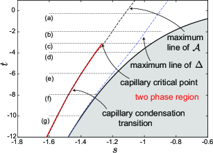
Figure 10: (Color online) Phase diagram of a near-critical fluid in a film for large adsorption in the $s$-$t$ plane, where $s=\psi_{\infty}/\psi_{D}(\propto\psi_{\infty}D^{\beta/\nu})$ and $t=\tau(D/\xi_{0})^{1/\nu}$. Two-phase region is written in the right (in gray). There appears a first-order phase transition line (red) of capillary condensation with a critical point at $(s,t)=(-1.27,-3.14)$. Plotted also are a line of maximum of $\Delta(s,t)$ with $(\partial\Delta/\partial s)_{t}=0$ and a line of maximum of ${\cal A}(s,t)$ (broken lines). The former approaches the coexistence curve for $t\lesssim-6$ and the latter is very close to the capillary condensation line. On paths (a)-(g), $m$, $\Gamma$, $\cal A$, and $\Delta$ are shown in Figs.11 and 12.

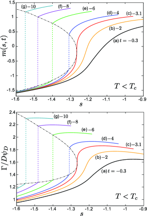
Figure 11: (Color online) Normalized midpoint order parameter $m=\psi(D/2)/\psi_{D}$ (top) and normalized excess adsorption $\Gamma/\psi_{D}D$ (bottom) vs $s$ in a film with thickness $D$ for $t=-0.3,-2,-3.1,-4,-6,-8$, and $-10$ from the right. See Eqs.(2.34) and (2.35) for $\Gamma$. For $t<-3.1$, these quantities are discontinuous across the capillary condensation line in Fig.10.

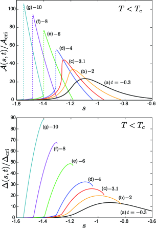
Figure 12: (Color online) Casimir amplitude ratios ${\cal{A}}(s,t)/{\cal{A}}_{\rm cri}$ (top) and $\Delta(s,t)/\Delta_{\rm cri}$ (bottom) vs $s$ for $t=-0.3,-2,-3.1,-4,-6,-8$, and $-10$ from the right. in the range $s<-\psi_{\rm cx}/\psi_{D}=-0.66|t|^{\beta}$. Curves (c) corresponds to the capillary-condensation critical point. Those (d)-(g) exhibit a first-order phase transition, where ${\cal A}$ is discontinuous but $\Delta$ is continuous.

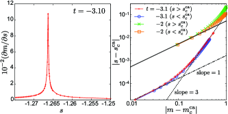
Figure 13: (Color online) Left: Susceptibility $(\partial m/\partial s)_{t}=(\partial\psi_{m}/\partial\psi_{\infty})_{\tau}$ at $t=-3.1$ slightly above the capillary-condensation critical point ($t_{c}^{\rm ca}=-3.14$). Right: Relations between deviations $s-s_{c}^{\rm ca}$ and $m-m_{c}^{\rm ca}$ near the capillary-condensation critical point at $t=-3.1$ and away from it at $t=-2$ on a logarithmic scale. The former can be fitted to the mean-field form (3.48).

We now discuss the phase behavior in the region of $t<0$ and $\psi_{\infty}<0$. In Fig.10, we show a first-order phase transition line in the region $t<0$ and $s<0$ outside the coexistence curve. As in Fig.11, the discontinuities of the physical quantities across this line decrease with increasing $t$ and vanish at a critical point $(\tau,\psi_{\infty})=(\tau_{c}^{\rm ca},\psi_{c}^{\rm ca})$. In agreement with the scaling theory Nakanishi-s , we obtain

$$\tau_{c}^{\rm ca}=-3.14(\xi_{0}/D)^{1/\nu},$$ (3.46)

$$\psi_{c}^{\rm ca}=-1.27\psi_{D}\cong-1.87b_{\rm cx}(\xi_{0}/D)^{\beta/\nu}.$$ (3.47)

We use the second line of Eq.(3.28) in Eq.(3.47). For $\tau<\tau_{c}^{\rm ca}$, let us write the transition point as $\psi_{\infty}=\psi_{\rm ca}(\tau)$ or as $s=s_{\rm ca}(t)=\psi_{\rm ca}(\tau)/\psi_{D}$. This line divides the condensed phase with $m>0$ in the range $s_{\rm ca}<s<-\psi_{\rm cx}/\psi_{D}$ and the noncondensed phase with $m<0$ in the range $s<s_{\rm ca}$. In Fig.11, the isothermal curves of $m=\psi(D/2)/\psi_{D}$ and $\Gamma/D\psi_{D}$ are shown as functions of $s$ for $t<0$, where they are continuous for $t>t_{c}^{\rm ca}=-3.14$ and discontinuous for $t<t_{c}^{\rm ca}$. It is the capillary condensation line for the gas-liquid transition Evansreview ; Gelb and is also the two-dimensional transition line for Ising-like films JSP ; Evans-Marconi ; Nakanishi-s ; Nakanishi-mean .

In Fig.10, we also plot two dotted lines. On one line, ${\cal A}(s,t)$ takes a maximum as a function of $s$ at fixed $t$. For $t<t_{c}^{\rm ca}$, it is slightly separated from the transition line for $t>-4.0$ but coincides with the transition line for $t<-4.0$. On the other line close to the bulk coexistence curve, $\Delta(s,t)$ takes a maximum as a function of $s$ at fixed $t$ and we have $(\partial\Delta/\partial s)_{t}=0$ and $\Gamma^{*}=0$ from Eq.(3.42).

In Fig.12, we plot the Casimir amplitudes ${\cal A}(s,t)$ and $\Delta(s,t)$ as functions of $s$ for $t<0$. For $t<t_{c}^{\rm ca}$, they grow very strongly in the condensed phase. As a marked feature, ${\cal A}$ and $\Delta$ behave very differently for $t<0$, though they behave similarly for $t>0$ in Fig.9. These results are consistent with their derivatives with respect to $s$ in Eqs.(3.41) and (3.42). Previously, enhancement of $\cal A$ was found close to the transition line in the condensed phase by Maciołek et al. Evans-Anna in two-dimensional Ising films and by Schlesener et al. JSP in the mean-field theory.

In Fig.11, the slope $(\partial m/\partial s)_{t}$ or the susceptibility $dm/ds$ in Eq.(2.32) diverges as $t$ is decreased to $t_{c}^{\rm ca}$. Thus, in Fig.13, we plot $(\partial m/\partial s)_{t}$ vs $s$ for $t=-3.1$ in the left panel and the curve of $m$ vs $s$ at $t=-3.1$ and -2 in the right panel. The curve of $t=-3.1$ can well fitted to the following mean-field form,

$$s-s_{c}^{\rm ca}=A_{\rm ca}(t-t_{c}^{\rm ca})(m-m_{c}^{\rm ca})+B_{\rm ca}(m-m_{c}^{\rm ca})^{3},$$ (3.48)

where $(t_{c}^{\rm ca},s_{c}^{\rm ca},m_{c}^{\rm ca})=(-3.14,-1.27,-0.172)$, $A_{\rm ca}=0.0425$, and $B_{\rm ca}=0.11$. This mean-field behavior near the capillary-condensation critical point arises because the long wavelength fluctuations of $\psi$ inhomogeneous in the lateral plane have been neglected. The curve of $t=-2$ is not well fitted to Eq.(3.48) for $|m-m_{c}^{\rm ca}|\gtrsim 0.3$.

III.6 Determination of the capillary condensation line

In Fig.14, we show the profile $\psi(z)$ at $t=-4$ for four values of $s$ given by (A) $-1.10$, (B) -1.29, (C) $-1.33$, and (D) -1.50, where $\psi_{0}=20\psi_{D}$. The two lines $\psi=\pm\psi_{\rm cx}$ are also shown, between which $|\psi|<\psi_{\rm cx}$ and the free energy density is given by the mean-field form (3.31). Here, between (B) and (C), there is a first-order phase transition at $s=-1.31$, where the normalized midpoint value $m$ changes discontinuously between $0.407$ and $-0.793$.

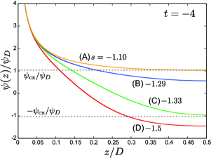
Figure 14: (Color online) Normalized order parameter $\psi(z)/\psi_{D}$ vs $z/D$ in a film in the half region $0<z<D/2$ at $t=-4$, with $\psi_{0}=20\psi_{D}$ in the symmetric boundary conditions. From above, (A) $s=-1.10$ (at maximum of $\Delta$), (B) -1.29 (near maximum of $\cal A$), (C) $-1.33$, and (D) $-1.50$. A first-order phase transition occurs between (B) and (C). Lines of $\psi_{\infty}=\pm\psi_{\rm cx}$ are written, where $\psi_{\rm cx}/\psi_{D}=1.04$.

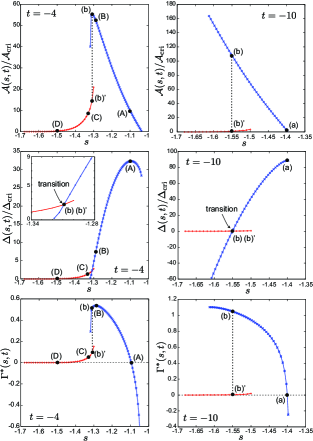
Figure 15: (Color online) ${\cal{A}}(s,t)/{\cal{A}}_{\rm cri}$ (top), $\Delta(s,t)/\Delta_{\rm cri}$ (middle), and $\Gamma^{*}(s,t)$ (bottom) for $t=-4$ (left) and $t=-10$ (right). For $t=-4$, points (A), (B), (C), and (D) correspond to the curves in Fig.14. There are equilibrium and metastable branches near the transition. Amplitude $\Delta$ is maximized at (A) (left) and at (a) (right), where $\Gamma^{*}=0$ from Eq.(3.42). The transition occurs between (b) and (b’), where $\Delta$ is continuous.

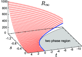
Figure 16: (Color online) Scaled inverse susceptibility for a film $R_{\infty}$ in Eqs.(2.52) and (3.42) in the $s$-$t$ plane, which is of order $40|s|^{\delta-1}$ for $|s|\gtrsim 1$.

In Fig.15, ${\cal{A}}(s)/{\cal{A}}_{\rm cri}$, $\Delta(s)/\Delta_{\rm cri}$, and $\Gamma^{*}$ are displayed as functions of $s$ at $t=-4$ (left) and -10 (right), where $\psi(z)$ for the points (A), (B), (C), and (D) at $t=-4$ can be seen in Fig.14. In numerical analysis, we obtained two branches of the profiles giving rise to hysteretic behavior at the transition. From Eq.(2.49) $\Delta$ should be maximized in equilibrium. Thus the equilibrium (metastable) branch should be the one with a larger (smaller) $\Delta$. A first-order phase transition occurs at a point where the two curves of $\Delta(t)$ cross. We confirm the following. (i) In accord with Eq.(3.42), the maximum point of $\Delta$ coincides with the vanishing point of $\Gamma^{*}$, as can be known from comparison of the middle and bottom panels. (ii) As $s\to-\psi_{\rm cx}/\psi_{D}$, ${\cal A}$ becomes very small on the top plates, since it approaches the value on the critical pass $\mu_{\infty}=0$ with $t<0$ displayed in Fig. 8 (see the sentence below Eq.(3.44)). (iii) As $s$ is decreased from $-\psi_{\rm cx}/\psi_{D}$ to the transition value $s_{\rm ca}$ in the condensed phase, ${\cal A}$ grows with a steep negative slope. To understand this behavior, we compare the first and second terms in the right hand side of Eq.(3.41). We notice that the ratio of the first term to the second is very small in this $s$ range. It is between $[0.02,0.05]$ for $t=-4$ and between $[0.001,0.005]$ for $t=-10$. In the condensed phase in the range $s_{\rm ca}<s<-\psi_{\rm cx}/\psi_{D}$, we thus find

$$\frac{\partial\cal A}{\partial s}\cong-R_{\infty}(m-s).$$ (3.49)

While $m-s$ remains of order $\psi_{\rm cx}/\psi_{D}\sim|t|^{\beta}$, the coefficient $R_{\infty}$ is very large outside the coexistence curve. Figure 16 displays the overall behavior of $R_{\infty}$ in the $s$-$t$ plane, where $R_{\infty}\cong 6.6|t|^{\gamma}$ on the coexistence curve and $R_{\infty}\cong A_{c}\delta(1+\delta)|s|^{\delta-1}\sim 40|s|^{\delta-1}$ for $|s|>1$.

We also comment on the validity of the general relation (3.43) in our numerical analysis. For example, at $t=-4$ in Fig.15, let us consider the two points (A) $s=-1.1$ and (B) $s=-1.29$. At point (A), we have ${\cal A}=5.54$, $\Delta=9.02$, $\partial\Delta/\partial s=3.13$, and $\partial\Delta/\partial t=-2.21$. The three terms in the right hand side of Eq.(3.43) are thus $18.04$, $1.78$, and $-14.03$ in this order and indeed their sum gives $\cal A$. At point (B), we have ${\cal A}=23.98$, $\Delta=1.98$, $\partial\Delta/\partial s=72.4$, and $\partial\Delta/\partial t=-3.85$, so the three terms in the right hand side of Eq.(3.43) are $3.96$, $-24.4$, and $48.2$ in this order, whose sum indeed yields $\cal A$.

IV Summary and remarks

We have calculated the order parameter profiles and the Casimir amplitudes for a film of near-critical fluids. Our results are also applicable to one-component fluids near the gas-liquid critical point where the walls favor either of gas or liquid. We summarize our main results.
(i) In Sec.II, we have used the singular free energy by Fisher and Au Yang at $T=T_{c}$. Using this model, we have defined the two Casimir amplitudes, $\cal A$ for the force density and $\Delta$ for the grand potential, as functions of the scaled order parameter of the reservoir $s=\psi_{\infty}/\psi_{D}$ in Eq.(3.31), They are sharply peaked at $s\sim-1$ and the peak heights are much larger than their critical-point values ${\cal A}_{\rm cri}$ and ${\Delta}_{\rm cri}$ as in Fig.4. These singular behaviors have been analyzed analytically. This off-critical behavior may also be interpreted as pretransitional enhancement, because the region of $s\sim-1$ and $t=0$ is close to the capillary-condensation critical point.
(ii) In Sec.III, we have constructed a free energy with the gradient contribution for $T\neq T_{c}$ including the renormalization effects, with which we may readily calculate the physical quantities. The Casimir amplitudes $\cal A$ and $\Delta$ are much amplified for $s\sim-1$ as shown in Fig.9 for $T>T_{c}$ and in Fig.12 for $T<T_{c}$. Their maxima are larger than their critical-point values by 10-100 times. We have then found a first-order phase transition line of capillary condensation for negative $t$ slightly outside the bulk coexistence curve, where the profile of $\psi$ and $\cal A$ are discontinuous but $\Delta$ is continuous. This line ends at a critical point given by $(s,t)=(-1.27,-3.14)$. The amplitude $\cal A$ exhibits a maximum close to this line, while the amplitude $\Delta$ close to the bulk coexistence curve.

We make some remarks.
1) Even at the mean-field level, it follows the power-law form of the interaction free energy $\Delta F$ for $\xi>D>\ell_{0}$:

$$\Delta F=-k_{B}T_{c}D^{-4}\Delta_{0}.$$ (4.1)

Here, setting $\delta=3$ in Eq.(2.3) and $\eta=0$ in Eq.(2.4), we obtain $\Delta_{0}=4I_{0}^{4}C_{0}^{2}/3B_{0}k_{B}T_{c}$ at the criticality under strong adsorption, where $I_{0}$ is given by Eq.(2.45). The adsorption-induced interaction is already present in the mean-field theoryOkamoto ; Tsori and its form becomes universal near the criticality Casimir . Enhancement of $\Delta F$ near the capillary condensation transition is rather obvious in view of the fact that it occurs even in the mean-field theory JSP . Note that $\Delta F\propto h_{1}^{2}$ for weak adsorption $(\ell_{0}>D$) away from the criticality, where $h_{1}$ is the surface field Okamoto .
2) We have neglected the fluctuations varying in the lateral plane with wavelengths longer than the three-dimensional $\xi$. Thus the capillary condensation transition has been treated at the mean-field level, leading to Fig.13. In idealized conditions, there should be composition-dependent crossovers from the Ising behavior in three dimensions to that in two dimensions.
3) Nucleation and spinodal decomposition should take place between plates and in porous media if $T$ is changed across the capillary condensation line outside the solvent coexistence curve Evansreview ; Gelb .
4) For neutral colloids, the attractive interaction arises from overlap of composition deviations near the colloid surfaces. It is intensified if the component favored by the surfaces is poor in the reservoir. A bridging transition further takes place at lower $\tau$ between strongly adsorbed or wetting layers of colloid particles Evans-Hop ; Nature2008 ; Okamoto .
5) Our local functional theory has been used when $\psi$ varies over a wide range in strong adsorption. It can be used in various situations. For example, dynamics of colloid particles in near-critical fluids can be studied including the hydrodynamic flow. So far, phase separation in near-critical fluids has been investigated in the scheme of the $\psi^{4}$ theory with constant renormalized coefficients Onukibook . However, the distance to the bulk criticality (the parameter $w$ in Sec.III) can be inhomogeneous around preferential walls or around heated or cooled walls.
6) We should further investigate the ion effects in confined multi-component fluids. In such situations, the surface ionization can depend on the ambient ion densities and composition Current ; Okamoto . A prewetting transition then appears even away from the solvent coexistence curve, where the degree of ionization is also discontinuous. We are interested in how the ionization fluctuations affect the ion-induced capillary condensation transition Tsori .

Appendix A: Mechanical equilibrium

In one-dimensional situations, the $zz$ component of the stress tensor due to the composition deviation is Onukibook

$$\Pi_{zz}=\psi\mu-f+C(|\psi^{\prime}|^{2}/2-\psi\psi^{\prime\prime})-C^{\prime}\psi|\psi^{\prime}|^{2}/2,$$ (A1)

where $C^{\prime}=dC/d\phi$. The mechanical equilibrium condition is $d\Pi_{zz}/dz=0$, so $\Pi_{zz}$ is a constant independent of $z$. We further use Eq.(2.11) to eliminate the term proportional to $\psi^{\prime\prime}$ to obtain

$$\Pi_{zz}=\psi\mu_{\infty}-f+C|\psi^{\prime}|^{2}/2.$$ (A2)

Thus $\Pi_{zz}=\psi_{m}\mu_{\infty}-f_{m}$ at $z=D/2$. The osmotic pressure is given by

$$\Pi=\Pi_{zz}-(\psi_{\infty}\mu_{\infty}-f_{\infty}),$$ (A3)

so we find $\Pi=-\partial\Omega/\partial D$ in Eq.(2.39).

Appendix B: Relationship to the Schofield, Lister, and Ho linear parametric model

The linear parametric model Sc69 provides the equation of state and thermodynamic quantities of Ising systems in compact forms Hohenberg ; Wallace2 for detailed discussions on this model. It uses two parametric variables, $\hat{r}$ and $\theta$, with $\hat{r}\geq 0$ and $|\theta|\leq 1$; $\hat{r}$ represents a distance to the critical point and $\theta$ an angle around it in the $\psi$-$\tau$ plane. Here $\hat{r}$ should not be confused with $r$ in Eq.(3.5). In this model, homogeneous equilibrium states are supposed. The reduced temperature $\tau$, the magnetic field $h$, and the average order parameter $\psi$ are expressed in terms of $\hat{r}$ and $\theta$ as

$$\tau = {\hat{r}}(1-b_{c}^{2}\theta^{2}),$$ (B1)

$$h = a_{0}\hat{r}^{\beta\delta}\theta(1-\theta^{2}),$$ (B2)

$$\psi = c_{0}{\hat{r}}^{\beta}\theta.$$ (B3)

Here $a_{0}$ and $c_{0}$ are positive nonuniversal constants, while $b_{c}$ is a universal number. The case $\theta=0$ corresponds to $\tau>0$ and $h=0$, $\theta=\pm 1/b_{c}$ to $\tau=0$, and $\theta=\pm 1$ to the coexistence curve ($h=0$ and $\tau<0$). We may calculate various thermodynamic quantities from these relations in agreement with the asymptotic critical behavior. Though $b_{c}$ is arbitrary within the model, $b_{c}^{2}$ was set equal to

$$b_{c}^{2}=(\delta-3)/[(\delta-1)(1-2\beta)]\cong 1.36.$$ (B4)

This choice yields simple expressions for the critical amplitude ratios in close agreement with experiments. The linear parametric model in Eqs.(B1)-(B4) is exact up to order $\epsilon^{2}$ Wallace2 . The two-scale-factor universality Stauffer ; HAHS furthermore indicates that the combination $(a_{0}c_{0})\xi_{0}^{d}$ of the coefficients in Eqs.(B2) and (B3) should be a universal number, where $\xi_{0}$ is the microscopic length in the correlation length $\xi=\xi_{0}\tau^{-\nu}$ for $\tau>0$ and $h=0$.

Our model in Eqs.(3.4)-(3.9) closely resemble the liner parametric model as regards the thermodynamics of homogeneous states. Note that $h$ in Eq.(B2) corresponds to $\mu/k_{B}T$ in Eq.(3.20) and $\hat{r}$ to $w$ in Eq.(3.9). For our model, we may introduce the angle variable $\theta$ by

$$\theta={\rm sign}(\psi)b_{O}^{-1}\sqrt{1-S},$$ (B5)

where $S$ is defined in Eq.(3.17). We set $\theta=\pm 1$ on the coexistence curve so that

$$b_{O}^{2}={1+1/\sigma}\cong 1.58,$$ (B6)

where $\sigma$ is given by Eq.(3.22). Then $\tau$, $\mu$, and $\psi$ are expressed in terms of $w$ and $\theta$ as

$$\tau=w(1-b_{O}^{2}\theta^{2}),$$ (B7)

$$\frac{\mu}{k_{B}T}=C_{3}w^{\beta\delta}\theta(1-\theta^{2})\frac{1-A_{1}\theta^{2}}{1-A_{2}\theta^{2}},$$ (B8)

$$\psi=(b_{O}/\sqrt{C_{2}})w^{\beta}\theta,$$ (B9)

where the coefficients $A_{1}$, $A_{2}$, and $C_{3}$ are expressed as

$$A_{1} = 5\alpha b_{O}^{2}/[5\alpha+(2-\alpha)\sigma]\cong 0.23,$$ (B10)

$$A_{2} = (1-2\beta)b_{O}^{2}\cong 0.55,$$ (B11)

$$C_{3} = b_{O}^{2}[5\alpha+(2-\alpha)\sigma]C_{1}/[6\sqrt{C_{2}}\xi_{0}^{2}].$$ (B12)

As differences between our model and the linear parametric model, $b_{O}^{2}$ in Eq.(B6) is larger than $b_{c}^{2}$ in Eq.(B3) by $16\%$ and there appears the extra factor,

$$Z(\theta)=({1-A_{1}\theta^{2}})/({1-A_{2}\theta^{2}}),$$ (B13)

in the right hand side of Eq.(B8). Our model considerably deviates from the parametric model close to the coexistence curve mainly because of $Z(1)=1.73$. The correlation length $\xi$ and the susceptibility $\chi^{-1}$ on the coexistence curve are thus underestimated in our theory as in Eqs.(3.26) and (3.27). Also in our model the combination $C_{3}(b_{0}/\sqrt{C_{2}})\xi_{0}^{d}$ for the coefficients in Eqs.(B8) and (B9) is a universal number from Eq.(3.11) in accord with the two-scale-factor universality.

References

- (1) R. Evans, J. Phys.: Condens. Matter 2, 8989 (1990).
- (2) L.D. Gelb, K.E. Gubbins, R. Radhakrishnan, and M. Sliwinska-Bartkowiak, Rep. Prog. Phys. 62, 1573 (1999).
- (3) J. W. Cahn, J. Chem. Phys. 66 3667 (1977).
- (4) P.G. de Gennes, Rev. Mod. Phys. 57, 827 (1985).
- (5) D. Chandler, Nature 437, 640 (2005).
- (6) A. Onuki and H. Kitamura, J. Chem. Phys. 121, 3143 (2004).
- (7) A. Onuki, R. Okamoto, and T. Araki, Bull. Chem. Soc. Jpn. 84, 569 (2011); A. Onuki and R. Okamoto, Current Opinion in Colloid Interface Science 16, 525 (2011).
- (8) R. Okamoto and A. Onuki, Phys. Rev. E 84, 051401 (2011).
- (9) M. E. Fisher and H. Nakanishi, J. Chem. Phys. 75, 5857 (1981).
- (10) H. Nakanishi and M. E. Fisher, J. Chem. Phys. 78, 3279 (1983).
- (11) R. Evans and U. M. B. Marconi, J. Chem. Phys. 86, 7138 (1987).
- (12) A. Maciołek, A. Drzewiński,and R. Evans, Phys. Rev. E 64, 056137 (2001); A. Drzewiński, A. Maciołek, and A. Barasiński, Mol. Phys. 109, 1133 (2011).
- (13) Binary mixtures are characterized by the temperature and the chemical potential difference betwen the two components at a constant pressure . In the text, in the resevoir, where is the critical value.
- (14) S. Samin and Y. Tsori, EPL 95, 36002 (2011).
- (15) M.E. Fisher and P.G. de Gennes, C. R. Acad. Sci. Paris Ser. B 287 207 (1978).
- (16) M. E. Fisher and H. Au-Yamg, Physica 101A, 255 (1980). In their paper the gradient part of the free energy density is proportional to . In the present paper we set .
- (17) H. Nakanishi and M.E. Fisher, Phys. Rev. Lett. 49, 1565 (1982).
- (18) K. Binder, in Phase Transitions and Critical Phenomena, C. Domb and J. L. Lebowitz, eds. (Academic, London, 1983), Vol. 8, p. 1.
- (19) S. Dietrich, in Phase Transitions and Critical Phenomena, edited by C. Domb and J. L. Lebowitz (Academic, London, 1988), Vol. 12, p. 1.
- (20) J.O. Indekeu, M.P. Nightingale and W.V. Wang, Phys. Rev. B 34, 330 (1986).
- (21) M. Krech and S. Dietrich, Phys. Rev.A 46, 1886 (1992).
- (22) M. Krech, J. Phys.: Condens. Matt. 11, R391 (1999).
- (23) M. Krech, Phys. Rev. E 56, 1642 (1997).
- (24) F. Schlesener, A. Hanke, and S. Dietrich, J. Stat. Phys. 110, 981 (2003). Figure 10 of this paper shows the scaling function for the force density at for a film.
- (25) O. Vasilyev, A. Gambassi, A. Maciołek, and S. Dietrich, EPL 80, 60009 (2007).
- (26) A. Gambassi, A. Maciołek, C. Hertlein, U. Nellen, L. Helden, C. Bechinger, and S. Dietrich, Phys. Rev. E 80, 061143 (2009).
- (27) Z. Borjan and P. J. Upton, Phys. Rev. Lett. 81, 4911 (1998).
- (28) Z. Borjan and P. J. Upton, Phys. Rev. Lett. 101, 125702 (2008).
- (29) M. Hasenbusch, Phys. Rev. B 82, 174434 (2010).
- (30) The long-range interaction () in near-critical binary mixtures treated in this paper arises from the slow and universal composition decay in the fluid induced by the wall perturbation. From our viewpoint, it is somewhat misleading to call it the Casimir interaction, though we use ”Casimir amplitudes”. The Casimir interaction itself was originally found to be induced by the ground-state fluctuations of the electromagnetic field between two mirrors.
- (31) A. Mukhopadhyay and B.M. Law, Phys. Rev. Lett. 83, 772 (1999); R. Garcia and M.H.W. Chan, Phys. Rev. Lett. 83, 1187 (1999); A. Mukhopadhyay and B. M. Law, Phys. Rev. E 63, 041605 (2001).
- (32) B. M. Law, Prog. Surf. Sci. 66, 159 (2001).
- (33) S. Rafai, D. Bonn, and J. Meunier, Physica A 386, 31 (2007).
- (34) P. Hopkins, A.J. Archer, and R. Evans, J. Chem. Phys. 131, 124704 (2009).
- (35) D. Beysens and D. Estve, Phys. Rev. Lett. 54, 2123 (1985); B.M. Law, J.-M. Petit, and D. Beysens, Phys. Rev. E, 57, 5782(1998); D. Beysens and T. Narayanan, J. Stat. Phys. 95, 997 (1999).
- (36) P. D. Gallagher and J. V. Maher, Phys. Rev. A 46, 2012 (1992); P. D. Gallagher, M. L. Kurnaz, and J. V. Maher, Phys. Rev. A 46, 7750 (1992).
- (37) Y. Jayalakshmi and E. W. Kaler, Phys. Rev. Lett. 78, 1379 (1997).
- (38) H. Guo, T. Narayanan, M. Sztucki, P. Schall and G. Wegdam, Phys. Rev. Lett. 100, 188303 (2008)
- (39) D. Bonn, J. Otwinowski, S. Sacanna, H. Guo, G. Wegdam and P. Schall, Phys. Rev. Lett. 103, 156101 (2009).
- (40) C. Hertlein, L. Helden, A. Gambassi, S. Dietrich, and C. Bechinger, Nature 451, 172 (2008).
- (41) U. Nellen, J. Dietrich, L. Helden, S. Chodankar, K. Nygard, J. Friso van der Veen, and C. Bechinger, Soft Matter 7, 5360 (2011).
- (42) Z. Borjan and P. J. Upton, Phys. Rev. E 63, 065102(R) (2001).
- (43) A. Onuki, Phase Transition Dynamics (Cambridge University Press, Cambridge, 2002).
- (44) D. Stauffer, D. Ferer and M. Wortis, Phys. Rev. Lett. 29, 345 (1972).
- (45) P.C. Hohenberg, A. Aharony, B.I. Halperin and E.D. Siggia, Phys. Rev. B 13, 2986 (1976).
- (46) J. Rudnick and D. Jasnow, Phys. Rev. Lett. 48, 1059 (1982); ibid. 49, 1595 (1982)
- (47) P. Schofield, Phys. Rev. Lett. 22, 606 (1969); P. Schofield, J.D. Lister, and J.T. Ho, ibid. 23, 1098 (1969).
- (48) P. C. Hohenberg and M. Barmatz, Phys. Rev. A 6, 289 (1972). In this paper, explicit expressions were presented for the Helmholtz free energy and the entropy in the linear parametric model (but outside the coexistence curve).
- (49) D.J. Wallace, in Phase Transitions and Critical Phenomena, vol.6, ed C. Domb C and J.L. Lebowitz (Academic Press, London, 1976), p.294.
- (50) M. E. Fisher and P. J. Upton, Phys. Rev. Lett. 65, 3405 (1990); M. E. Fisher, S.-Y. Zinn, and P.J. Upton, Phys. Rev. B 59, 14533 (1999).
- (51) The singular free energy density is of the form for and , where is a universal number of order 0.1 Onukibook ; HAHS . Twice differentiating with respect to , we obtain the well-known specific heat .
- (52) J.F. Nicoll and P.C. Albright, Phys. Rev. B 31, 4576 (1985).
- (53) A. J. Liu and M. E. Fisher, Physica A 156, 35 (1989).
- (54) M.R. Moldover, Phys. Rev. A 31, 1022 (1985); T. Mainzer and D. Woermann, Physica A 225, 312 (1996).
- (55) The susceptibility is given by , where .
- (56) G. Flöter and S. Dietrich, Z. Phys. B 97, 213 (1995).