Nonconventional averages
along arithmetic progressions
and lattice spin systems

Abstract

We study the so-called nonconventional averages in the context of lattice spin systems, or equivalently random colourings of the integers. For i.i.d. colourings, we prove a large deviation principle for the number of monochromatic arithmetic progressions of size two in the box $[1,N]\cap\mathbb{N}$, as $N\to\infty$, with an explicit rate function related to the one-dimensional Ising model.
For more general colourings, we prove some bounds for the number of monochromatic arithmetic progressions of arbitrary size, as well as for the maximal progression inside the box $[1,N]\cap\mathbb{N}$.
Finally, we relate nonconventional sums along arithmetic progressions of size greater than two to statistical mechanics models in dimension larger than one.

1 Introduction

Nonconventional averages along arithmetic progressions are averages of the type

$$\frac{1}{N}\sum_{i=1}^{N}f_{1}(X_{i})f_{2}(X_{2i})\cdots f_{k}(X_{\ell i})$$ (1)

where $(X_{n})$ is a sequence of random variables, and $f_{1},\ldots,f_{\ell}$ are bounded measurable functions.

Motivation to study such averages comes from the study of arithmetic progressions in subsets of the integers, and multiple recurrence and multiple ergodic averages. In that context, typically $X_{i}=T^{i}(x)$, with $T$ a weakly mixing transformation, and $x$ is distributed according to the unique invariant measure. See e.g. [9, 1, 11] for more background on this deep and growing field.

Only recently, starting with the work of Kifer [14], and Kifer and Varadhan [15], central limit behavior of nonconventional averages was considered. These authors consider averages along progressions more general than the arithmetic ones. It is natural to consider the averages of the type (1) from a probabilistic point of view and ask questions such as whether they satisfy a large deviation principle, whether associated extremes have classical extreme value behavior, etc.

These questions are far from obvious, since even in the simplest case of $f_{i}$ being all identical, the sum

$$S_{N}=\sum_{i=1}^{N}\prod_{j=1}^{\ell}f(X_{ji})$$

is quite far from a sum of shifts of a local function. In particular it is highly non-translation invariant. From the point of view of statistical mechanics, large deviations of $S_{N}/N$ are related to partition function and free energy associated to the “Hamiltonian” $S_{N}$. Since $S_{N}$ is not translation-invariant and (extremely) long-range, even the existence of the associated free energy is not obvious.

In this paper, we restrict to random variables $X_{i}$ taking values in a finite set. For the sake of definiteness, we assume the joint distribution to be a Gibbs measure with an exponentially decaying interaction to obtain fluctuation properties of $S_{N}$ in a straightforward way. In Section 3 we obtain some basic probabilistic properties using Gaussian concentration and Poincaré’s inequality which are available for the Gibbs measures we consider.
In Section 4, we explicitly compute the large deviation rate function of $\frac{1}{N}\sum_{i=1}^{N}X_{i}X_{2i}$ when the $X_{i}$’s are i.i.d. Bernoulli random variables. Even if this is the absolute simplest setting, the rate function turns out to be an interesting non-trivial object related to the one-dimensional Ising model. Recently there has been a lot of interest in multifractal analysis of non-conventional ergodic averages [12, 13, 16, 7, 8]. Large deviation rate functions are often related to multifractal spectra of conventional ergodic averages. In the present context, this connection is not as straightforward as it is in the context of sums of shifts of a local function. We expect the results of this paper to be useful in establishing such connection in the context of non-conventional averages.

Finally, we analyze in the last section the case of arithmetic progressions of size larger than two. This naturally leads to statistical mechanics models in dimension higher than one, possibly having phenomenon of phase transitions. Conversely the classical Ising model in dimension $d>1$ can be related to specific unconventional sums, which we describe below. Such a connection deserves future investigations.

2 The setting

We consider $K$-colorings of the integers and denote them as $\sigma,\eta,$ elements of the set of configurations $\Omega=\{0,\ldots,K\}^{\mathbb{Z}}$. We assume that on $\Omega$ there is a translation-invariant Gibbs measure with an exponentially decaying interaction, denoted by $\mathbb{P}$. This means that, given $\alpha\in\{0,\ldots,K\}$, for the one-site conditional probability

$$\varphi_{\hat{\sigma}}(\alpha)=\mathbb{P}(\sigma_{0}=\alpha|\sigma_{\mathbb{Z}\setminus\{0\}}=\hat{\sigma})$$

we assume the variation bound

$$\|\varphi_{\hat{\sigma}}-\varphi_{\hat{\eta}}\|_{\infty}\leq e^{-n\rho}$$

for some $\rho>0$ whenever $\hat{\sigma}$ and $\hat{\eta}$ agree on $[-n,n]\cap\{{\mathbb{Z}\setminus\{0\}}\}$. This class of measures is closed under single-site transformations, i.e., if we define new spins $\sigma^{\prime}_{i}=F(\sigma_{i})$ with $F:\{0,1,\ldots,K\}\to\{0,1\ldots,K^{\prime}\}$, $K^{\prime}<K$, then $\mathbb{P}^{\prime}$, the image measure on $\{0,1\ldots,K^{\prime}\}^{\mathbb{Z}}$, is again a Gibbs measure with exponentially decaying interaction, see e.g. [17] for a proof. In the last section, we restrict to product measures.

For the rest of the paper we consider only $2$-colorings (i.e. $K=1$). Given an integer $\ell$, we are interested in the random variable

$$\sum_{i=1}^{N}\prod_{j=1}^{\ell}\sigma_{ji}$$

which counts the number of arithmetic progressions of size $\ell$ with “colour” $1$ (starting from one) in the block $[1,Nk]$.

If we consider $K$-colorings and monochromatic arithmetic progressions, i.e., random variables of the type

$$\sum_{i=1}^{N}\prod_{j=1}^{\ell}\mathds{1}(\sigma_{ji}=\alpha)$$

for given $\alpha\in\{0,\ldots,K\}$, then we can define the new “colors” $\sigma^{\prime}_{i}=\mathds{1}(\sigma_{i}=\alpha)$ which are zero-one valued and, as stated before, are distributed according to $\mathbb{P}^{\prime}$, a Gibbs measure with an exponentially decaying interaction. Therefore, if we restrict to monochromatic arithmetic progressions, there is no loss of generality if we consider $2$-colorings.

Define the averages

$${\mathcal{A}}^{\ell}_{N}=\frac{1}{N}\sum_{i=1}^{N}\prod_{j=1}^{\ell}\sigma_{ji}.$$

Several natural questions can be asked about them and about some related quantities. We give here a non-exhaustive list. Questions 1 and 2 on this list have been answered positively in the literature in a much more general context (see [9] for question 1 and [14, 15] for question 2). On the contrary questions 3 and 4 have not been considered before.

1. Law of large numbers: Does ${\mathcal{A}}^{\ell}_{N}$ converge to $(\mathbb{E}(\sigma_{0}))^{\ell}$ as $N\to\infty$ with $\mathbb{P}$ probability one ?

2. Central limit theorem: Does there exist some $a^{2}>0$ such that

   $$\sqrt{N}\big{(}{\mathcal{A}}^{\ell}_{N}-\left(\mathbb{E}(\sigma_{0})\right)^{\ell}\big{)}\operatorname{\stackrel{{\scriptstyle\scriptscriptstyle\rm law}}{{\longrightarrow}}}{\cal N}(0,a^{2}),\,\textup{as}\,N\to\infty\,?$$

3. Large deviations: Does the rate function

   $$I(x)=\lim_{\epsilon\to 0}\lim_{N\to\infty}-\frac{1}{N}\log\mathbb{P}\left({\mathcal{A}}^{\ell}_{N}\in[x-\epsilon,x+\epsilon]\right)$$

   exist and have nice properties ? In view of the Gärtner-Ellis theorem [6], the natural candidate for $I$ is the Legendre transform of the “free-energy”

   $${\mathcal{F}}(\lambda)=\lim_{N\to\infty}\frac{1}{N}\log\mathbb{E}\big{(}e^{N\lambda{\mathcal{A}}^{\ell}_{N}}\big{)}$$

   provided this limit exists and is differentiable. If, additionally, ${\mathcal{F}}$ is analytic in a neighborhood of the origin, then the central limit theorem follows [3].

4. Statistics of nonconventional patterns. Let

   $${\mathcal{M}}(N)=$$

   $$\qquad\max\{k\in\mathbb{N}:\exists\;1\leq i\leq N/k\ \text{such that}\ \sigma_{i}=1,\sigma_{2i}=1,\ldots,\sigma_{ki}=1\}$$

   be the maximal arithmetic progression of colour $1$ starting from zero in the block $[1,N]$. One would expect

   $${\mathcal{M}}(N)\approx C\log N+X_{N}$$

   where $0<C<\infty$ and $X_{N}$ is a tight sequence of random variables with an approximate Gumbel distribution, i.e.,

   $$e^{-c_{1}e^{-x}}\leq\mathbb{P}\left(X_{N}\leq x\right)\leq e^{-c_{2}e^{-x}}.$$

   Related to this is the exponential law for the occurence of “rare arithmetic progressions”: Let

   $${\mathcal{T}}(\ell)=\inf\{n\in\mathbb{N}:\exists\;1\leq i\leq n/\ell\ \text{such that}\ \sigma_{i}=1,\sigma_{2i}=1,\ldots,\sigma_{\ell i}=1\}$$

   be the smallest block $[1,n]$ in which a monochromatic arithmetic progression can be found with size $k$. Then one expects that ${\mathcal{T}}(\ell)$, appropriately normalized, has approximately (as $\ell\to\infty$) an exponential distribution. Finally, another convenient quantity is

   $${\mathcal{K}}(N,\ell)=\sum_{i=1}^{\lfloor N/\ell\rfloor}\prod_{j=1}^{\ell}\sigma_{ji}=\lfloor N/\ell\rfloor{\mathcal{A}}^{\ell}_{\lfloor N/\ell\rfloor}$$

   which counts the number of monochromatic arithmetic progressions of size $\ell$ inside $[1,N]$.
   The probability distributions of these quantities are related by the following relations:

   $$\mathbb{P}({\mathcal{K}}(N,\ell)=0)=\mathbb{P}({\mathcal{M}}(N)<\ell)=\mathbb{P}({\mathcal{T}}(\ell)>N)\;.$$

3 Some basic probabilistic properties

In this section we prove some basic facts about the nonconventional averages considered in the previous section.

PROPOSITION 3.1.

2. Gaussian concentration bound. Let $\ell\geq 1$ be an integer. There exists a constant $C>0$ such that for all $n\geq 1$ and all $t>0$

   $$\mathbb{P}\left(\left|{\mathcal{A}}_{N}^{\ell}-\mathbb{E}\left({\mathcal{A}}_{N}^{\ell}\right)\right|>t\right)\leq e^{-CNt^{2}}.$$ (2)

   In particular, ${\mathcal{A}}_{N}^{\ell}$ converges almost surely to $\left(\mathbb{E}(\sigma_{0})\right)^{\ell}$ as $N$ goes to infinity.

3. Logarithmic upper bound for maximal monochromatic progressions. There exists $\gamma>0$ such that for all $c>\gamma$

   $${\mathcal{K}}(N,c\log N)\to 0$$

   in probability as $N\to\infty$.

PROOF.  A Gibbs measure for an exponentially decaying interaction satisfies both the Gaussian concentration bound (see e.g. [4]), and the Poincaré inequality [5]. For a bounded measurable function $f:\Omega\to\mathbb{R}$ let

$$\nabla_{i}f(\sigma)=f(\sigma^{i})-f(\sigma)$$

be the discrete derivative at $i\in\mathbb{Z}$, where $\sigma^{i}$ is the configuration obtained from $\sigma\in\Omega$ by flipping the symbol at $i$. Next define the variation

$$\delta_{i}f=\sup_{\sigma}\nabla_{i}f(\sigma)$$

and

$$\|\delta f\|_{2}^{2}=\sum_{i\in\mathbb{Z}}(\delta_{i}f)^{2}.$$

Then, on the one hand, we have the Gaussian concentration inequality: there exists some $c_{1}>0$ such that

$$\mathbb{P}\left(|f-\mathbb{E}(f)|>t\right)\leq e^{-\frac{c_{1}t^{2}}{\|\delta f\|_{2}^{2}}}$$ (3)

for all $f$ and $t>0$. On the other hand, we have the Poincaré inequality: there exists some $c_{2}>0$ such that

$$\mathbb{E}\left[(f-\mathbb{E}f)^{2}\right]\leq c_{2}\sum_{i\in\mathbb{Z}}\int(\nabla_{i}f)^{2}\textup{d}\mathbb{P}$$ (4)

for all $f$. Now choosing

$$f={\mathcal{A}}_{N}^{\ell}$$

we easily see that

$$\|\delta f\|_{2}^{2}\leq\ell^{2}/N\;.$$

This combined with (3) gives (2). To see that this implies almost-sure convergence to $\mathbb{E}(\sigma_{0})^{\ell}$, we use the strong mixing property enjoyed by one-dimensional Gibbs measures with exponentially decaying interacting [10, Chap. 8], from which it follows easily that

$$|\mathbb{E}(\sigma_{ki}|\sigma_{ri},r\not=k)-\mathbb{E}(\sigma_{0})|\leq Ce^{-ci}$$

which implies

$$|\mathbb{E}(\sigma_{i}\sigma_{2i}\cdots\sigma_{\ell i})-\mathbb{E}(\sigma_{0})^{\ell}|\leq C_{\ell}\,e^{-ci}$$

This in turn implies

$$\lim_{N\to\infty}\mathbb{E}({\mathcal{A}}^{\ell}_{N})=\mathbb{E}(\sigma_{0})^{\ell}.$$

Combining this fact with (2) yields the almost-sure convergence of ${\mathcal{A}}^{\ell}_{n}$ towards $\mathbb{E}(\sigma_{0})^{\ell}$ as $n$ goes to infinity. The first statement is thus proved.

In order to prove the second statement, we use the bound

$$\mathbb{E}\left(\prod_{j=1}^{q}\sigma_{i_{j}}\right)\leq e^{-\gamma q}$$ (5)

for some $\gamma>0$ and for all $i_{1},\ldots,i_{q}\in\mathbb{Z}$. This follows immediately from the ‘finite-energy property’ of one-dimensional Gibbs measures, i.e., the fact that there exists $\delta\in(0,1)$ such that for all $\sigma\in\Omega,\alpha\in\{0,1\}$

$$\delta<\mathbb{P}\left(\sigma_{0}=\alpha|\sigma_{\mathbb{Z}\setminus\{0\}}\right)<1-\delta.$$

As a consequence,

$$\left|\nabla_{j}\left(\prod_{r=1}^{\ell}\sigma_{ir}\right)\right|\leq\mathds{1}(j\in\{i,2i,\ldots,\ell i\})\prod_{r=1,ri\not=j}^{\ell}\sigma_{ri}$$

and hence, using the elementary inequality $(\sum_{i=1}^{N}a_{i})^{2}\leq N\sum_{i=1}^{n}a_{i}^{2}$, we have the upper bound

$$\left|\nabla_{j}{\mathcal{K}}(N,\ell)\right|^{2}\leq N\sum_{i=1}^{\lfloor N/\ell\rfloor}\prod_{r=1}^{\ell}\sigma_{ir}\mathds{1}(j\in\{i,2i,\ldots,\ell i\}).$$

Integrating against $\mathbb{P}$, using (5) and summing over $j$ yields

$$\sum_{j}\int\left(\nabla_{j}{\mathcal{K}}(N,\ell)\right)^{2}\textup{d}\mathbb{P}\leq N^{2}e^{-\ell\gamma}\;.$$

Choosing now

$$\ell=\ell(N)=c\log N,$$

and using (4), we find

$$\textup{Var}({\mathcal{K}}(N,\ell(N)))\leq CN^{2-c\gamma}\;.$$

Hence, for $\gamma>2/c$, the variance of ${\mathcal{K}}(N,c\log N)$ converges to zero. Since

$$\mathbb{E}({\mathcal{K}}(N,\ell(N))\leq N\,e^{-\gamma k}\leq N^{1-c\gamma},$$

the expectation of ${\mathcal{K}}(N,\ell(N))$ also converges to zero, hence we have convergence to zero in mean square sense and thus in probability. $\;\qed$

4 Large deviations for arithmetic progressions of size two

From the point of view of functional inequalities such as the Gaussian concentration bound or the Poincaré inequality, there is hardly a difference between sums of shifts of a local function, i.e. conventional ergodic averages, and their nonconventional counterparts.

The difference becomes however manifest in the study of large deviations. If we think e.g. about $\sum_{i=1}^{N}\sigma_{i}\sigma_{i+1}$ versus $\sum_{i=1}^{N}\sigma_{i}\sigma_{2i}$ as “Hamiltonians” then the first sum is simply a nearest neighbor translation-invariant interaction, whereas the second sum is a long-range non translation invariant interaction. Therefore, from the point of view of computing partition functions, the second Hamiltonian will be much harder to deal with.

In this section we restrict to the product case, by choosing $\mathbb{P}_{p}$ to be product of Bernoulli with parameter $p$ on two symbols $\{+,-\}$, and consider arithmetic progressions of size two $(k=2)$. We will show that the thermodynamic limit of the free energy function associated to the sum

$$S_{N}=\sum_{i=1}^{N}\sigma_{i}\sigma_{2i}$$

defined as

$${\mathcal{F}}_{p}(\lambda)=\lim_{N\to\infty}\frac{1}{N}\log\mathbb{E}_{p}\left(e^{\lambda S_{N}}\right)$$ (6)

exists, is analytic as a function of $\lambda$ and has an explicit expression in terms of combinations of Ising model partition functions for different volumes.

To start, assuming $N$ to be odd (the case $N$ even is treated similarly), we make the following useful decomposition

$$S_{N}=\sum_{l=1}^{\frac{N+1}{2}}S_{l}^{(N)}$$

with

$$S_{l}^{(N)}=\sum_{i=0}^{M_{l}(N)-1}\sigma_{(2l-1)2^{i}}\sigma_{(2l-1)2^{i+1}}$$ (7)

and

$$M_{l}(N)=\left\lfloor\log_{2}\left(\frac{N}{2l-1}\right)\right\rfloor+1\;.$$

where $\lfloor x\rfloor$ denotes the integer part of $x$. The utility of such decomposition is that the random variable $S_{l}^{(N)}$ is independent from $S_{l^{\prime}}^{(N)}$ for $l\neq l^{\prime}$. A similar decomposition into independent blocks has also been used independently in [7, 8]. This implies that the partition function in the free energy (6) will factorize over different subsystems labeled by $l\in\{1,\ldots,(N+1)/2\}$, each of size $M_{l}(N)+1$. Therefore we can treat separately each variable $S_{l}^{(N)}$.

Furthermore, defining new spins

$$\tau_{i}^{(l)}=\sigma_{(2l-1)2^{i-1}}\qquad\text{for}\quad i\in\{1,\ldots,M_{l}(N)+1\}\;,$$

it is easy to realize that, for a given $l\in\{1,\ldots,(N+1)/2\}$, the variable $S_{l}^{(N)}$ is nothing else than the Hamiltonian of a one-dimensional nearest-neighbors Ising model, since

$$\{S_{l}^{(N)}\}\stackrel{{\scriptstyle\mathcal{D}}}{{=}}\left\{\sum_{i=1}^{M_{l}(N)}\tau^{(l)}_{i}\tau^{(l)}_{i+1}\right\}$$

where $\tau^{(l)}_{i}$ are Bernoulli random variables with parameter $p$, independent for different values of $l$ and for different values of $i$ and $\stackrel{{\scriptstyle\mathcal{D}}}{{=}}$ denotes equality in distribution. Introduce the notation

$${\mathcal{Z}}(\lambda,h,n+1)=\sum_{\tau\in\{-1,1\}^{n+1}}e^{\lambda\sum_{i=1}^{n}\tau_{i}\tau_{i+1}+h\sum_{i=1}^{n+1}\tau_{i}}$$

for the partition function of the one-dimensional Ising model with coupling strength $\lambda$ and external field $h$ in the volume $\{1,\ldots,n\}$, with free boundary conditions. Then we have

$$\mathbb{E}_{p}\left(e^{\lambda\sum_{i=1}^{n}\tau_{i}\tau_{i+1}}\right)=(p(1-p))^{\frac{n+1}{2}}{\mathcal{Z}}(\lambda,h,n+1)$$ (8)

with $h=\frac{1}{2}\log(p/(1-p))$. A standard computation (see for instance [2], Chapter 2) gives

$${\mathcal{Z}}(\lambda,h,n+1)=v^{T}M^{n}v=|v^{T}\cdot e_{+}|^{2}\Lambda_{+}^{n}+|v^{T}\cdot e_{-}|^{2}\Lambda_{-}^{n}$$

with $\Lambda_{\pm}$ the largest, resp. smallest eigenvalue of the transfer matrix (with elements $M_{\alpha,\beta}=e^{\lambda\alpha\beta+\frac{h}{2}(\alpha+\beta)}$), i.e.,

$$\Lambda_{\pm}=e^{\lambda}\left(\cosh(h)\pm\sqrt{\sinh^{2}(h)+e^{-4\lambda}}\right),$$

$v^{T}$ the vector with components $(e^{h/2},e^{-h/2})$, $e_{\pm}$ the normalized eigenvectors corresponding to the eigenvalues $\Lambda_{\pm}$.

Using the decomposition (7), we obtain from (8)

$$\log\mathbb{E}_{p}\left(e^{\lambda S_{N}}\right)=\sum_{l=1}^{(N+1)/2}\log\left(p(1-p)^{\frac{M_{l}(N)+1}{2}}{\mathcal{Z}}(\lambda,h,M_{l}(N)+1)\right).$$

Furthermore, observing that

$$\lim_{N\to\infty}\frac{1}{N}\sum_{l=1}^{(N+1)/2}M_{l}(N)=\frac{1}{2}\int\psi(x)\textup{d}x$$

with

$$\psi(x)=\left\lfloor\log_{2}\left(\frac{1}{x}\right)\right\rfloor+1\;,$$

we obtain

$${\mathcal{F}}_{p}(\lambda) =\frac{1}{4}\left(\int\psi(x)\textup{d}x+1\right)\log(p(1-p))$$

$$\quad+\frac{1}{2}\int_{0}^{1}\log\left(|v^{T}\cdot e_{+}|^{2}\Lambda_{+}^{\psi(x)}+|v^{T}\cdot e_{-}|^{2}\Lambda_{-}^{\psi(x)}\right)\textup{d}x.$$

To obtain a more explicit formula one can make use of the following: the normalized eigenvector corresponding to the largest eigenvalue is

$$e_{+}=\frac{w_{+}}{\|w_{+}\|}$$

with

$$w_{+}=\left(\begin{array}[]{c}-e^{-\lambda}\\ e^{h+\lambda}-\Lambda_{+}\end{array}\right)$$

and moreover

$$|v^{T}\cdot e_{-}|^{2}=\|v\|^{2}-|v^{T}\cdot e_{+}|^{2}=2\cosh(h)-|v^{T}\cdot e_{+}|^{2}\;.$$

Since $\psi(x)=n+1$ for $x\in(1/2^{n+1},1/2^{n}]$, we have

$$\int\psi(x)\textup{d}x=2\;,$$

hence one gets

$${\mathcal{F}}_{p}(\lambda)=\log\left([p(1-p)]^{\frac{3}{4}}|v^{T}\cdot e_{+}|\;\Lambda_{+}\right)+{\mathcal{G}}(\lambda)$$ (9)

with

$${\mathcal{G}}(\lambda)=\frac{1}{2}\sum_{n=1}^{\infty}\frac{1}{2^{n}}\log\left(1+\left(\frac{2\cosh(h)}{|v^{T}\cdot e_{+}|^{2}}-1\right)\left(\frac{\Lambda_{-}}{\Lambda_{+}}\right)^{n}\right)\;.$$

In the case $p=1/2$, we have $h=0$, $\Lambda_{+}=e^{\lambda}+e^{-\lambda}$, $|v^{T}\cdot e_{+}|^{2}=\|v\|^{2}=2$ which implies ${\mathcal{G}}(\lambda)=0$ and

$${\mathcal{F}}_{1/2}(\lambda)=\log\left(\frac{1}{2}\left(e^{\lambda}+e^{-\lambda}\right)\right)\;.$$ (10)

One recognizes in this case the Legendre transform of the large deviation rate function for a sum of i.i.d. bernoulli $(1/2)$ because (only) in this case $p=1/2$ the joint distribution of $\{\sigma_{i}\sigma_{2i},i\in\mathbb{N}\}$ coincides with the joint distribution of a sequence of independent Bernoulli$(1/2)$ variables. When $p\not=1/2$, although an explicit formula is given in (9), the expression reflects the multiscale character of the decomposition and it is non-trivial.

As a consequence of the explicit formula (9), we have the following

THEOREM 4.1.

1. Large deviations. The sequence of random variables $\frac{S_{N}}{N}$ satisfies a large deviation principle with rate function

   $$I_{p}(x)=\sup_{\lambda\in\mathbb{R}}\left(\lambda x-{\mathcal{F}}_{p}(\lambda)\right)$$

   where ${\mathcal{F}}_{p}(\lambda)$ is given by (9).

2. Central limit theorem. The sequence of random variables

   $$N^{-1/2}\left(S_{N}-\mathbb{E}_{p}(S_{N})\right)$$

   weakly converges to a Gaussian random variable with strictly positive variance $\sigma^{2}={\mathcal{F}}_{p}^{\prime\prime}(0)>0$.

PROOF.  The expression (9) shows that ${\mathcal{F}}_{p}$ is differentiable as a function of $\lambda$, hence the first statement follows from the Gärtner-Ellis theorem [6]. The second statement follows from the fact that ${\mathcal{F}}_{p}$ is analytic in a neighborhood of the origin, which again follows directly from the explicit expression. $\;\qed$

REMARK 4.1.

The value $p=1/2$ is special since in this case the joint distribution of $\{\sigma_{i}\sigma_{2i},i\in\mathbb{N}\}$ coincides with the joint distribution of a sequence of independent $\textup{Bernoulli}(1/2)$ variables. Therefore we must have

$$I_{1/2}(x)=\begin{cases}\frac{1}{2}(1+x)\log\left(1+x\right)+\frac{1}{2}(1-x)\log\left(1-x\right)&\text{ if }|x|\leq 1\;,\\ +\infty&\text{ if }|x|>1\;.\end{cases}$$

This can be checked by computing ${\mathcal{F}}_{1/2}$ as done above (see (10)). We must also have $\sigma^{2}=1$ for $p=1/2$.

REMARK 4.2.

Notice that we computed the large deviation rate function in the $\pm 1$ setting. If one considers a Bernoulli measure ${\mathbb{Q}}_{p}$ on $\{0,1\}^{\mathbb{Z}}$, with ${\mathbb{Q}}_{p}(\eta_{i}=1)=p$, then the large deviations of the sums

$$\sum_{i=1}^{N}\eta_{i}\eta_{2i}$$ (11)

correspond to the large deviations of

$$\frac{1}{4}\sum_{i=1}^{N}(1+\sigma_{i})(1+\sigma_{2i})=\frac{1}{4}\left(N+\sum_{i=1}^{N}(\sigma_{i}+\sigma_{2i})+\sum_{i=1}^{N}\sigma_{i}\sigma_{2i}\right)$$

where $\sigma$ is distributed according to $\mathbb{P}_{p}$ on $\{+,-\}^{\mathbb{Z}}$. In particular, the free energy for the large deviations of (11) under the measure ${\mathbb{Q}}_{1/2}$ corresponds to a free energy of the $\sigma$ spins with non-zero magnetic field and hence can again be computed explicitly.

REMARK 4.3.

A plot of the free energy for a few values of $p$ is shown in Figure 1 (it is enough to analyze values in $(0,1/2]$ since ${\mathcal{F}}_{p}(\lambda)={\mathcal{F}}_{1-p}(\lambda)$).

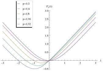
Figure 1: Plot of the free energy function for different $p$ values. The graph has been obtained from formula (9) truncating the sum to the first 100 terms.

In the general case $p\neq 1/2$ it is interesting to compare our results to the independent case. To this aim one consider the sum $\sum_{i=1}^{N}\xi_{i}\eta_{i}$ where $\xi_{i},\eta_{i}$ are two sequences of i.i.d. Bernoulli of parameter $p$. Note that in this case the family $\{\xi_{i}\eta_{i}\}_{i\in\{1,\ldots,N\}}$ is made of independent Bernoulli random variables with parameter $p^{2}+(1-p)^{2}$. An immediate computation of the free energy yields on this case

$$\mathcal{F}_{p}^{(\textup{ind})}(\lambda)=\log\left([p^{2}+(1-p)^{2}]e^{\lambda}+2p(1-p)e^{-\lambda}\right)$$ (12)

This free energy is compared to that of formula (9) in Figure 2.

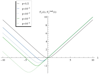
Figure 2: Plot of the free energy function (9) (continuous line) and of the free energy of the independent case (12) (dashed line).

In particular one can analyze the behaviour of the minimum of the free energy functions in the two cases, corresponding to the negative value of the large deviation rate function computed at zero. This is shown in Figure 3, which suggests a general inequality between the two cases.

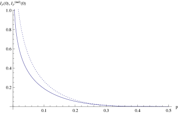
Figure 3: The negative of the minimum of the free energy as a function of $p$ for the two cases (9) and (12).

5 Size larger than two and Ising model in higher dimension

In this Section we analyze the case of arithmetic progressions of size larger than two. Such a case naturally leads to statistical mechanics models in dimension higher than one, possibly having phenomenon of phase transitions. Conversely the classical Ising model in dimension $d>1$ can be related to specific unconventional sums, which we describe below.

5.1 Decompositions for $k\geq 2$

When the size of the arithmetic progressions is larger than two ($k>2$), we have sums of the type

$$S_{N}=\sum_{i=1}^{N}\sigma_{i}\sigma_{2i}\cdots\sigma_{ki}\;,$$

where $\sigma_{i}$ are i.i.d. random variables taking values in the set $\{-1,+1\}$. One can try to decompose this sum into independent sums as it was done in Section 4. After relabeling the indices one obtains independent sums, each of which corresponds to a spin system with Hamiltonian in a bounded domain of $\mathbb{N}^{d_{k}}$, where the dimension $d_{k}$ is given by the number of prime numbers contained in the set $\{2,\ldots,k\}$. Denoting by $p_{1},p_{2},\ldots,p_{d_{k}}$ the prime numbers contained in $\{2,\ldots,k\}$ and defining

$$A^{(N)}_{p}:=\{m\in\{2,\ldots,N\}\,:\;m\>\text{ is not divisible by }\>p\}$$

and

$$A^{(N)}_{p_{1},\ldots,p_{d_{k}}}:=\bigcap_{l=1}^{d_{k}}A_{p_{l}}^{(N)}\;$$

then one has the following decomposition:

$$S_{N}=\sum_{m\in A^{N}_{p_{1},\ldots,p_{d_{k}}}}S_{m}^{(N)}\;.$$

The independent sums $S_{m}^{(N)}$ are given by translation-invariant Hamiltonians of the form

$$S_{m}^{(N)}=\sum_{X\subset\mathbb{N}^{d_{k}}}J_{X}^{(m)}\tau_{X}^{(m)}$$

where the spins $\tau_{X}^{(m)}$ are given by

$$\tau_{X}^{(m)}=\prod_{{j}\in X}\tau_{{j}}^{(m)}:=\prod_{(j_{1},j_{2},\ldots,j_{d_{k}})\in X}\sigma_{m\,p_{1}^{j_{1}}\,p_{2}^{j_{2}}\cdots p_{d_{k}}^{j_{k}}}$$

and the couplings $J_{X}^{(m)}$ are

$$J_{X}^{(m)}=\begin{cases}1&\text{if }X=T_{l}X(k)\quad\text{for some}\quad{l}\in\Lambda_{p_{1},\ldots,p_{d_{k}}}^{m}(N)\\ 0&\text{otherwise}\end{cases}$$

with

$$\Lambda_{p_{1},\ldots,p_{d_{k}}}^{m}(N)=\left\{0,1,\ldots,\left\lfloor\log_{p_{1}}\frac{N}{m}\right\rfloor\right\}\times\cdots\times\left\{0,1,\ldots,\left\lfloor\log_{p_{d_{k}}}\frac{N}{m}\right\rfloor\right\}\subset\mathbb{N}^{d_{k}}\,,$$

$T_{l}X$ the translation of the set $X$ by the vector $l$, and $X(k)$ a specific subset of $\mathbb{N}^{d_{k}}$ depending on the size of the arithmetic progression $k$. This set $X(k)$ is a polymer starting at the origin and having $k$ vertices. The specific shape of $X(k)$ sets the range of interaction along each direction of the $d_{k}-$dimensional lattice. In general the shape of the interaction depends on the non-prime numbers contained in $\{2,\ldots,k\}$.

We clarify this construction with a few examples.

• $k=2$

  $$\sum_{i=1}^{N}\sigma_{i}\sigma_{2i}=\sum_{m\in A_{2}^{(N)}}\sum_{i\in\Lambda_{2}^{m}(N)}\sigma_{m\cdot 2^{i}}\>\sigma_{m\cdot 2^{i+1}}=\sum_{m\in A_{2}^{(N)}}\sum_{i\in\Lambda_{2}^{m}(N)}\tau_{i}^{(m)}\tau_{i+1}^{(m)}\;.$$

  This Hamiltonian is the 1-dimensional nearest-neighbor Ising model of Section 4 constructed from the basic polymer $X(2)=\{0,1\}$.

• $k=3$

  $$\sum_{i=1}^{N}\sigma_{i}\sigma_{2i}\sigma_{3i} =\sum_{m\in A_{2,3}^{(N)}}\sum_{(i,j)\in\Lambda_{2,3}^{m}(N)}\sigma_{m\cdot 2^{i}3^{j}}\>\sigma_{m\cdot 2^{i+1}3^{j}}\>\sigma_{m\cdot 2^{i}3^{j+1}}$$

  $$=\sum_{m\in A_{2,3}^{(N)}}\sum_{(i,j)\in\Lambda_{2,3}^{m}(N)}\tau_{i,j}^{(m)}\,\tau_{i+1,j}^{(m)}\,\tau_{i,j+1}^{(m)}\;.$$

  This corresponds to a 2-dimensional nearest-neighbor model with triple interaction obtained via the polymer $X(3)=\{(0,0),(0,1),(1,0)\}$.

• $k=4$

  $$\sum_{i=1}^{N}\sigma_{i}\sigma_{2i}\sigma_{3i}\sigma_{4i} =\sum_{m\in A_{2,3}^{(N)}}\sum_{(i,j)\in\Lambda_{2,3}^{m}(N)}\>\sigma_{m\cdot 2^{i}3^{j}}\>\sigma_{m\cdot 2^{i+1}3^{j}}\>\sigma_{m\cdot 2^{i+2}3^{j}}\>\sigma_{m\cdot 2^{i}3^{j+1}}$$

  $$=\sum_{m\in A_{2,3}^{(N)}}\sum_{(i,j)\in\Lambda_{2,3}^{m}(N)}\tau_{i,j}^{(m)}\,\tau_{i+1,j}^{(m)}\,\tau_{i+2,j}^{(m)}\,\tau_{i,j+1}^{(m)}\;.$$

  This gives a 2-dimensional model sums with quadruple interaction constructed by translating the polymer $X(4)=\{(0,0),(1,0),(2,0),(0,1)\}$. The range of interaction is 2 in one direction and 1 in the other direction.

• $k=5$

  $$\sum_{i=1}^{N}\sigma_{i}\sigma_{2i}\sigma_{3i}\sigma_{4i}\sigma_{5i}$$

  $$=\sum_{m\in A_{2,3,5}^{(N)}}\sum_{(i,j,l)\in\Lambda_{2,3,5}^{m}(N)}\sigma_{m\cdot 2^{i}3^{j}5^{l}}\>\sigma_{m\cdot 2^{i+1}3^{j}5^{l}}\>\sigma_{m\cdot 2^{i+2}3^{j}5^{l}}\>\sigma_{m\cdot 2^{i}3^{j+1}5^{l}}\>\sigma_{m\cdot 2^{i}3^{j}5^{l+1}}$$

  $$=\sum_{m\in A_{2,3,5}^{(N)}}\sum_{(i,j,l)\in\Lambda_{2,3,5}^{m}(N)}\tau_{i,j,l}^{(m)}\,\tau_{i+1,j,l}^{(m)}\,\tau_{i+2,j,l}^{(m)}\,\tau_{i,j+1,l}^{(m)}\,\tau_{i,j,l+1}^{(m)}\;.$$

  Here we get a 3-dimensional model with quintuple interaction given by the basic polymer $X(5)=\{(0,0,0),(1,0,0),(2,0,0),(0,1,0),(0,0,1)\}$. The range of interaction is 2 in one direction and 1 in the other two directions.

5.2 Unconventional sums related to 2-dimensional Ising model

We consider now the standard 2-dimensional neirest-neighbor Ising model sums

$$\sum_{(i,j)\in\Lambda}\tau_{i,j}(\tau_{i+1,j}+\tau_{i,j+1})$$

in a domain $\Lambda$ of $\mathbb{N}^{2}$, and wonder whether there exist some unconventional averages that may be related to it through the decomposition procedure previously described. The answer is in the affirmative sense and is contained in the following two examples.

• For $\{\sigma_{i}\}_{i\in\mathbb{N}}$ a sequence of independent random variables taking values in $\{-1,+1\}$, we have

  $$\sum_{i=1}^{N}\sigma_{i}(\sigma_{2i}+\sigma_{3i}) =\sum_{m\in A_{2,3}^{(N)}}\sum_{(i,j)\in\Lambda_{2,3}^{m}(N)}\sigma_{m\cdot 2^{i}3^{j}}\>(\sigma_{m\cdot 2^{i+1}3^{j}}+\sigma_{m\cdot 2^{i}3^{j+1}})$$

  $$=\sum_{m\in A_{2,3}^{(N)}}\sum_{(i,j)\in\Lambda_{2,3}^{m}(N)}\tau_{i,j}^{(m)}\,(\tau_{i+1,j}^{(m)}+\tau_{i,j+1}^{(m)})$$

  with $\tau_{i,j}^{(m)}=\sigma_{m\cdot 2^{i}3^{j}}$. This clearly gives a decomposition into $|A_{2,3}^{(N)}|$ independent two-dimensional nearest-neighbor Ising sums.

• Let $\sigma_{i,j}$ be i.i.d. dichotomic random variables labeled by $(i,j)\in\mathbb{N}^{2}$. Then

  $$\sum_{i,j=1}^{N}\sigma_{i,j}(\sigma_{2i,j}+\sigma_{i,2j}) =\sum_{m\in A_{2}^{(N)}}\sum_{(i,j)\in\Lambda_{2}^{m}(N)}\sigma_{m\cdot 2^{i},m\cdot 2^{j}}\>\left(\sigma_{m\cdot 2^{i+1},m\cdot 2^{j}}+\sigma_{m\cdot 2^{i},m\cdot 2^{j+1}}\right)$$

  $$=\sum_{m\in A_{2}^{(N)}}\sum_{(i,j)\in\Lambda_{2}^{m}(N)}\nu_{i,j}^{(m)}\,(\nu_{i+1,j}^{(m)}+\nu_{i,j+1}^{(m)})$$

  with $\nu_{i,j}^{(m)}:=\sigma_{m\cdot 2^{i},m\cdot 2^{j}}$. We have a decomposition into $|A_{2}^{(N)}|$ independent two-dimensional nearest-neighbor Ising sums.

References

- [1] A. Arbieto, C. Matheus, C.G. Moreira, The remarkable effictiveness of ergodic theory in number theory, Ensaios Math., 17, 1–104, 2009.
- [2] R.J. Baxter, R.J., Exactly solved models in statistical mechanics, Academic Press London, 1982
- [3] W. Bryc, A remark on the connection between the large deviation principle and the central limit theorem, Stat. Prob. Letters, 18, 253-256, 1993.
- [4] J.-R. Chazottes, P. Collet, C. Külske, F. Redig, Concentration inequalities for random fields via coupling. Probab. Theory Related Fields 137, 201–225, (2007).
- [5] J.-R. Chazottes, P. Collet and F. Redig, Coupling, concentration and stochastic dynamics, J. Math. Phys. 49, Issue 12, paper number 125214 (2008).
- [6] A. Dembo, O. Zeitouni, Large Deviations, techniques and applications, Second edition, Springer, 1998
- [7] A. Fan, L. Liao, J.-H. Ma, Level sets of multiple ergodic averages, Preprint, ArXiv 1105.3032 (2011).
- [8] A. Fan, J. Schmeling, M. Wu, Multifractal analysis of multiple ergodic averages, C. R. Math. Acad. Sci. Paris 349 no. 17-18, 961 964, (2011)
- [9] H. Furstenberg, Recurrence in ergodic theory and combinatorial number theory, Princeton university press, Princeton, 1981.
- [10] H.-O. Georgii, Gibbs measures and phase transitions, de Gruyter Studies in Mathematics 9. Walter de Gruyter, Berlin, 2011 (2nd ed.).
- [11] B. Kra, From combinatorics to ergodic theory and back again. International Congress of Mathematicians. Vol. III, 57–76, Eur. Math. Soc., Zürich, 2006.
- [12] R. Kenyon, Y. Peres, B. Solomyak, Hausdorff dimension of the multiplicative golden mean shift, C. R. Math. Acad. Sci. Paris 349, no. 11-12, 625 628, (2011)
- [13] R. Kenyon, Y. Peres, B. Solomyak, Hausdorff dimension for fractals invariant under the multiplicative integers, Preprint, ArXiv 1102.5136 (2011).
- [14] Y. Kifer, Nonconventional limit theorems, Prob. Theory and Rel. Fields 148, 71-106, 2010.
- [15] Y. Kifer, S.R.S. Varadhan, Nonconventional limit theorems in discrete and continuous time via martingales. Preprint available at arxiv.org, 2010.
- [16] Y. Peres, B. Solomyak, Dimension spectrum for a nonconventional ergodic average, Preprint, ArXiv 1107.1749 (2011).
- [17] F. Redig and F. Wang, Transformations of one-dimensional Gibbs measures with infinite range interaction, Markov Processes and Rel. Fields, 16, 737-752, (2010).